High-Radix Floating-Point Division Algorithms for Embedded VLIW
单精度浮点算力 英文
单精度浮点算力英文Single-Precision Floating-Point ArithmeticThe field of computer science has witnessed remarkable advancements in the realm of numerical computation, with one of the most significant developments being the introduction of single-precision floating-point arithmetic. This form of numerical representation has become a cornerstone of modern computing, enabling efficient and accurate calculations across a wide range of applications, from scientific simulations to multimedia processing.At the heart of single-precision floating-point arithmetic lies the IEEE 754 standard, which defines the format and behavior of this numerical representation. The IEEE 754 standard specifies that a single-precision floating-point number is represented using 32 bits, with the first bit representing the sign, the next 8 bits representing the exponent, and the remaining 23 bits representing the mantissa or fraction.The sign bit determines whether the number is positive or negative, with a value of 0 indicating a positive number and a value of 1 indicating a negative number. The exponent field, which ranges from-126 to 127, represents the power to which the base (typically 2) is raised, allowing for the representation of a wide range of magnitudes. The mantissa, or fraction, represents the significant digits of the number, providing the necessary precision for accurate calculations.One of the key advantages of single-precision floating-point arithmetic is its efficiency in terms of memory usage and computational speed. By using a 32-bit representation, single-precision numbers require less storage space compared to their double-precision counterparts, which use 64 bits. This efficiency translates into faster data processing and reduced memory requirements, making single-precision arithmetic particularly well-suited for applications where computational resources are limited, such as embedded systems or mobile devices.However, the reduced bit-width of single-precision floating-point numbers comes with a trade-off in terms of precision. Compared to double-precision floating-point numbers, single-precision numbers have a smaller range of representable values and a lower level of precision, which can lead to rounding errors and loss of accuracy in certain calculations. This limitation is particularly relevant in fields that require high-precision numerical computations, such as scientific computing, financial modeling, or engineering simulations.Despite this limitation, single-precision floating-point arithmeticremains a powerful tool in many areas of computer science and engineering. Its efficiency and performance characteristics make it an attractive choice for a wide range of applications, from real-time signal processing and computer graphics to machine learning and data analysis.In the realm of real-time signal processing, single-precision floating-point arithmetic is often employed in the implementation of digital filters, audio processing algorithms, and image/video processing pipelines. The speed and memory efficiency of single-precision calculations allow for the processing of large amounts of data inreal-time, enabling applications such as speech recognition, noise cancellation, and video encoding/decoding.Similarly, in the field of computer graphics, single-precision floating-point arithmetic plays a crucial role in rendering and animation. The representation of 3D coordinates, texture coordinates, and color values using single-precision numbers allows for efficient memory usage and fast computations, enabling the creation of complex and visually stunning graphics in real-time.The rise of machine learning and deep neural networks has also highlighted the importance of single-precision floating-point arithmetic. Many machine learning models and algorithms can be effectively trained and deployed using single-precision computations,leveraging the performance benefits without significant loss of accuracy. This has led to the widespread adoption of single-precision floating-point arithmetic in the development of AI-powered applications, from image recognition and natural language processing to autonomous systems and robotics.In the field of scientific computing, the use of single-precision floating-point arithmetic is more nuanced. While it can be suitable for certain types of simulations and numerical calculations, the potential for rounding errors and loss of precision may necessitate the use of higher-precision representations, such as double-precision floating-point numbers, in applications where accuracy is of paramount importance. Researchers and scientists often carefully evaluate the trade-offs between computational efficiency and numerical precision when choosing the appropriate floating-point representation for their specific needs.Despite its limitations, single-precision floating-point arithmetic remains a crucial component of modern computing, enabling efficient and high-performance numerical calculations across a wide range of applications. As technology continues to evolve, it is likely that we will see further advancements in the representation and handling of floating-point numbers, potentially addressing the challenges posed by the trade-offs between precision and computational efficiency.In conclusion, single-precision floating-point arithmetic is a powerful and versatile tool in the realm of computer science, offering a balance between memory usage, computational speed, and numerical representation. Its widespread adoption across various domains, from real-time signal processing to machine learning, highlights the pivotal role it plays in shaping the future of computing and technology.。
Boosting very-high radix division with prescaling and selection by rounding
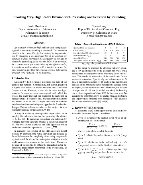
Boosting Very-High Radix Division with Prescaling and Selection by Rounding Paolo Montuschi Tom´a s Lang Dip.di Automatica e Informatica Dep.of Electrical and Computer Eng.Politecnico di Torino University of California at Irvine e-mail:montuschi@polito.it e-mail:tlang@AbstractAn extension of the very-high radix division with prescal-ing and selection by rounding is presented.This extension consists in increasing the effective radix of the implementa-tion by obtaining a few additional bits of the quotient per iteration,without increasing the complexity of the unit to obtain the prescaling factor nor the delay of an iteration. As a consequence,for some values of the effective radix, it permits an implementation with a smaller area and the same execution time than the original scheme.Estimations are given for54-bit and114-bit quotients.1.IntroductionDivision by digit recurrence produces one digit of the quotient per iteration.Consequently,for a given precision a higher radix results in fewer iterations and a potential faster execution.However,as the radix increases the digit-selection function becomes more complicated,which in-creases the cycle time and can overcome the reduction in execution time.Because of this,practical implementations are limited to up to radix-8stages and radix-16dividers have been implemented using overlapped radix-2and radix-4stages.Extensive literature exists on this subject;for spe-cific references see for instance[5,9,14]A way of achieving speedup with larger radices is to simplify the selection function by prescaling the divisor [4,8,10,17].In particular,prescaling and selection by rounding has been shown to produce a significant speedup [6].We refer to this scheme as the VHR approach,which has been extended to square root[12]andHere are shown improved values with respect to Table4in[6],since we used an improved linear approximation developed in[12]and[11].Table1.Execution time&area of VHR division Quotient bits per iteration9111418 Cycle time7.59.09.09.0 No.of cycles(54-bit quotient)10987 Execution time75817263 Area MAC520710740970 Area presc.factor module1302204701750:delay and area of full adder In this paper we increase the effective radix by obtain-ing a few additional bits of the quotient per cycle,while maintaining the complexity of the prescaling factor calcula-tion.This results in a reduction of the overall area for the same execution time.Specifically,we estimate that for54 bits,in the implementation for18quotient bits per iteration the area of the prescaling factor module plus the area of the multiplier,can be reduced by30%.Moreover,for the case of a quotient of114bits(extended precision)the boosting can achieve a speedup of about10%for the same area.We describe the algorithm,show the architecture,and estimate the improvement obtained with respect to VHR division. We assume familiarity with[5]and[6].2.Review of VHR divisionAs described in[6]in this approach the division is per-formed in the unit of Figure1,as followsCycle1:determine the scaling factor as an ap-proximation of such thatwhere is the divisor and the radix.Cycle2:obtain the scaled divisor(carry-save).Cycle3:obtain the initial residual(carry-save),where is the dividend.Assimilate.Cycles4toFigure1.Architecture of VHR division of[6] where is the(redundant)shifted residual trun-cated at the-th fractional bit,andThe residual is left in carry-save form.Cycle(3)as determined in Section4.1.The selection function has two components.Forwe perform selection by rounding,as done in[6].That is,(4) where is the truncation of the shifted residualto its th fractional bit.To allow this selection by rounding we need thatIn[5]the improved analytical expression(5)has been introduced,and it has been shown that it influences neither the analytical and numerical results nor the implementation of[6].very high radix division unitFigure 2.Proposed architectureThen(9)This means that the selection of corresponds to a radix-C division with replaced byand the restrictions(10)and(11)We first determine the digit set of and then the selec-tion function.4.1.Choice of digit set forIn this section we determine the digit set of .To do this,we need to determine bounds on the value of .We decompose as follows:(12)whereBecauseis selected by rounding we get(14)Consequently,the upper bound ofis(15)Note that we do not consider the special casesincethis produces ,as shown in [6].For the lower bound the worst case is produced by using,which can occur in the first iteration,leading to(17)Since the domain of is not symmetric,this results in anonsymmetric digit set for .Let us define the digit setWe start with the determination of the minimum ,which guarantees that (10)holds,i.e..From (9)we have that the worst-case situation occurs when is at its maximum value and has the minimum value of its domain;in this case,which results inNow should guarantee that. We have(20) Let us consider now the right hand side of(20).We have by expansion of,Now,for we have,(sinceSince should be an integer,we get as necessary and sufficient condition for the smallest value ofif(21) 4.2.Selection intervals and selection constantsWefirst determine the selection intervals and then use them to determine conditions for the selection constants. 4.2.1Selection intervalsSince the region of convergence of the algorithm is given by (10),we obtain,from(9),the following selection interval for.(22) However,the boosting algorithm should operate concur-rently with the VHR part,which implies that is not known.Consequently,we develop the selection function from instead of.Replacing byin(22)we get the bounds of the selection intervalsuch that if then can be se-lected.We get4.2.2Selection constantsNow,as in standard digit-recurrence division[5],the selec-tion function is described by the selection constants so that the value is selected if. Continuity requires that.As is, depends on and.Moreover,the selection requires knowledge of with full precision.Since there is over-lap between the selection intervals,it is possible to use esti-mates of these three quantities.If we call the estimate of and the estimate, we get(23) where the maximum and the minimum are determined for the range of values of and defined by the estimates and,respectively.This expression assumes with full precision.Estimate ofTo avoid the knowledge of with full precision,we use an estimate obtained from a few bits of the carry-save representation of,as follows.Sinceand is determined by rounding as described in(4),we obtain thatwhere is the-th digit of the representation of .That is,is the two’s complement repre-sentation of.Because of the way the rounding is per-formed and have values and the rest is in carry-save form.Consequently,the estimate of can be obtained from a truncated.Because of the two’s complement representation we getMoreover,if the truncation is done at the fractional bit,(24)Table2.Sufficient conditions for selection (bits of)(frac.bits of)As a consequence,when the estimate of is used, we get the selection intervals(25) and expression(23)is transformed to(26) where the*indicates the value larger than,with the granularity of.To determine suitable values of ,we need to specify the way the estimates and are computed.Estimate ofBecause of the selection by rounding,is directly de-rived from the most significant integer and2frac-tional bits of.We estimate by considering the most significant binary weights of,i.e.those from weight to weight.So,if the estimate is rep-resented in(assimilated)two’s complement representation while the rest of remains in carry-save representa-tion we getwhere(27) Consequently,from(4)it follows that(28) By combining(28)with(2),we get(29) Estimate and range ofSince,obtained from,is in two’s complement represen-tation we obtain(30) Moreover,since2.The generation of3.The incorporation of into the MAC4.The production ofConsequently,we now concentrate on the implementation of these blocks.Selection function ofAs described in Section4,the selection function requires the assimilation of parts of the carry-save representation of and then a function on the resulting bits.This im-plementation is shown in Figure3.Note the two-level as-similation required for,which is due to the fact that therounding to produce uses up to the the second fractional bit.Moreover,the estimate is obtained by a truncation of,which is produced by inverting the integer bit of.Of course,this inversion is not actually nec-essary to feed the selection function.Moreover,from(14) and as explained in section4.2.2on the range of,only the bit weights from weight to weight of enter the selection function.Generation of and residual updatingIn general,the generation of requires a rectangu-lar multiplier.This consists of two parts:generation of partial products and addition.The addition can be per-formed as part of the MAC tree,together with the updat-ing of the residual.For instance,for radix-4()sincetwo terms are required,unless the multiple is precomputed.Two terms are also required for. Incorporation into the MAC treeBecause the time of the selection function for is largerthan that for(done by rounding and recoding),to avoid that the boosting produces an increase in the cycle time,it is necessary to introduce the additional terms to lower lev-els of the MAC tree.This is possible if the original tree is not complete,as illustrated in Figure4.Since the MAC in the VHR division is used both for the recurrence and for the prescaling,the number of available slots at different levels depends on the radix and on the number of bits of the prescaling factor.Specifically,for the recurrence the num-ber of inputs to the tree is and for the prescal-ing,where is the number of fractional bits of the prescaling factor(since and must be represented,for recoding purposes,in two’s complement). Production ofFinally,it is necessary to producein two’s complement for the on-the-fly conversion.The im-plementation is simple and is not in the critical path.6.Evaluation and comparisonWe now give a rough estimation of the execution timeand the area of the boosting VHR division and compareFigure4.Levels of the MAC treewith VHR division.As was seen for the VHR scheme[6], the radices that have to be considered are the lowest that achieve a reduction in the number of cycles.Consequently, we need to compare the VHR with radix with the boost approach with.For the execution time we can give the following general considerations.The cycle time is determined by the maximum of the time to compute the prescaling factor and the time to perform an iteration of the recurrence.Moreover,the time to compute the scaling factor depends onfor the VHR approach and on for the boosting ap-proach.Consequently,this time might be reduced byusing the boosting approach.the time of an iteration is the same for both schemes,as long as the delay of the selection function forand the generation of the multiple is overlapped bythe recoding and rounding,the multiplexer,the mul-tiple generator,and thefirst levels of the MAC tree. Consequently,the addition of the boosting can produce a speedup if the delay of the calculation of the scaling factor is the critical component.This depends on the way this cal-culation is performed.The implementation model we use shows that it is reasonable to assume that the delay of this calculation is not critical.Consequently,for the same radix ,we do not expect the boosting to produce a speedup.With respect to the area,the main components are the MAC and the calculation of the prescaling factor.The area of the MAC increases somewhat when adding the boosting, because of the partitioning of the multiplier into two parts. On the other hand,the reduction in the area of the module to calculate the prescaling factor should be substantial,when going from to radix.This is the main advan-tage of the boosting technique.We now perform an estimate of this area reduction.6.1.Choice ofAcceptable values of are determined by the following considerations:Table3.Available slots in the MAC tree11-1215-1619-208101214-16slots321VHR+boost()---190021002900Area ratio0.800.650.55(a)114-bit quotientrecurrence and also on the number of bits of the prescalingfactor,which depends on the way this factor is computed[3,7,15,16,18].Using the L-approach described in[12](and,more in general in[11])we obtain that the numberof inputs to the tree required by the VHR division is.Consequently,the number of empty slots is shownin Table3.Therefore,since for and we needtwo slots,in the sequel we consider.6.3.Suitable values ofAs described in[13],the suitable values of depend onthe required precision of the quotient;namely,the suitablevalues are the smallest that produce a given number of cy-cles.These values for and bits(double andextended precision,respectively)are as reported in Table4.6.4.Execution time and areaTable5shows estimates of the execution time and areaof VHR division and of the version with boosting,using themodels presented in[12].As can be seen from the table,for54bits the boosting technique is only effective for,in which case the area ratio(VHR+boost)/(VHR)is0.7.On the other hand,for114bits it is effective forand,producing ratios between0.85and0.65.Moreover,for114bits we estimate that additionalarea reductions can be achieved by using.Figure5shows the tradeoff between area and speedup,using as reference values for delay and area the radix-2im-plementation as reported in[5],i.e.area equal toFigure5.Speedup vs.Area comparisonsand for54and114bits,respectively,and delay equal to and again for54and114bits,re-spectively.For54bits we estimate a VHR+boost() unit4times faster than the“classical”radix-2architecture, requiring6times its hardware;in this case,the estimated area saving is about30%,with respect to the VHR unit with the same delay.On the other hand,for114bits both very-high radix implementations produce speedups of up to6; the reduction in area of the implementations of the boosting algorithm being of25%(for C=4)and of35%(for C=8), with respect to the standard VHR implementation.More-over,from Table5b we observe that for114bits using an area of about,we can design either a VHR radix-unit with total delay of or a VHR+boost radix-unit(with)with total delay10%smaller.7.ConclusionsWe have presented an algorithm and implementation that increases the effective radix of the very-high radix division approach presented in[6].This is accomplished by obtain-ing a few additional bits of the quotient per iteration without increasing the complexity of the module to obtain the scal-ing factor,nor the iteration delay.We show that for some values of the effective radix this approach results in a significant reduction in the area of the module to compute the prescaling factor with respect to the original scheme.As a consequence,it is possible to achieve values of the execution time with a smaller unit.We expect this approach to be useful for other related operation such as square root andin a very high radix combined division/square-root unit withscaling.IEEE put.,C-47(2):152–161,February 1998.[2]Compass Design Automation.Passport-0.6Micron,3-Volt,High Performance Standard Cell pass Design Automation,Inc.,1994.[3] D.DasSarma and D.Matula.Faithful bipartite rom recipro-cal tables.In Proc.of the12th IEEE Symposium on Com-puter Arithmetic,pages12–25,Bath,England,July1995.[4]M.Ercegovac and ng.Simple radix-4division withoperands scaling.IEEE put.,C-39(9):1204–1208,September1990.[5]M.Ercegovac and ng.Division and Square Root:Digit-Recurrence Algorithms and Implementations.Kluwer Academic Press,New York,NJ,1994.[6]M.Ercegovac,ng,and P.Montuschi.Very high radixdivision with prescaling and selection by rounding.IEEE put.,C-43(8):909–917,August1994.[7]M.Ito,N.Takagi,and S.Yajima.Efficient initial approxi-mation for multiplicative division and square root by a mul-tiplication with operand modification.IEEE put., C-46(4):495–498,April1997.[8]J.Klir.A note on Svoboda’s algorithm for r-mation Processing Machines,(Stroje na Zpracovani Infor-maci),9:35–39,1963.[9]puter Arithmetic Algorithms.Prentice-Hall,Englewood Cliffs,NJ,1993.[10] E.Krishnamurthy.On range-transformation techniques fordivision.IEEE put.,C-19(2):157–160,February 1970.[11]ng and P.Montuschi.Improved methods to a linear in-terpolation approach for computing the prescaling factor for very high radix division.I.R.DAI/ARC6-94,Dipartimento di Automatica e Informatica,1994.[12]ng and P.Montuschi.Very high radix combined divi-sion and square root with prescaling and selection by round-ing.In Proc.of the12th IEEE Symposium on Computer Arithmetic,pages124–131,Bath,England,July1995. [13]P.Montuschi and ng.An algorithm for boosting veryhigh radix division with prescaling and selection by round-ing.I.R.DAI/ARC4-98,Dipartimento di Automatica e In-formatica,1998.[14]S.Oberman and M.Flynn.Division algorithms and imple-mentations.IEEE put.,C-46(8):833–854,Au-gust1997.[15]M.Schulte and J.Stine.Symmetric bipartite tables for ac-curate function approximation.In Proc.of the13th IEEE Symposium on Computer Arithmetic,pages175–183,Asilo-mar,CA,July1997.[16] E.Schwarz and M.Flynn.Hardware starting approxima-tion method and its application to the square root opera-tion.IEEE put.,C-45(12):1356–1369,Decem-ber1996.[17] A.Svoboda.An algorithm for division.Inf.Proc.Mach.,9:25–32,1963.[18]N.Takagi.Generating a power of an operand by a tablelookup and a multiplication.In Proc.of the13th IEEE Sym-posium on Computer Arithmetic,pages126–131,Asilomar, CA,July1997.。
XPSPEAK 说明书
Using XPSPEAK Version 4.1 November 2000Contents Page Number XPS Peak Fitting Program for WIN95/98 XPSPEAK Version 4.1 (1)Program Installation (1)Introduction (1)First Version (1)Version 2.0 (1)Version 3.0 (1)Version 3.1 (2)Version 4.0 (2)Version 4.1 (2)Future Versions (2)General Information (from R. Kwok) (3)Using XPS Peak (3)Overview of Processing (3)Appearance (4)Opening Files (4)Opening a Kratos (*.des) text file (4)Opening Multiple Kratos (*.des) text files (5)Saving Files (6)Region Parameters (6)Loading Region Parameters (6)Saving Parameters (6)Available Backgrounds (6)Averaging (7)Shirley + Linear Background (7)Tougaard (8)Adding/Adjusting the Background (8)Adding/Adjusting Peaks (9)Peak Types: p, d and f (10)Peak Constraints (11)Peak Parameters (11)Peak Function (12)Region Shift (13)Optimisation (14)Print/Export (15)Export (15)Program Options (15)Compatibility (16)File I/O (16)Limitations (17)Cautions for Peak Fitting (17)Sample Files: (17)gaas.xps (17)Cu2p_bg.xps (18)Kratos.des (18)ASCII.prn (18)Other Files (18)XPS Peak Fitting Program for WIN95/98 XPSPEAKVersion 4.1Program InstallationXPS Peak is freeware. Please ask RCSMS lab staff for a copy of the zipped 3.3MB file, if you would like your own copyUnzip the XPSPEA4.ZIP file and run Setup.exe in Win 95 or Win 98.Note: I haven’t successfully installed XPSPEAK on Win 95 machines unless they have been running Windows 95c – CMH.IntroductionRaymond Kwok, the author of XPSPEAK had spent >1000 hours on XPS peak fitting when he was a graduate student. During that time, he dreamed of many features in the XPS peak fitting software that could help obtain more information from the XPS peaks and reduce processing time.Most of the information in this users guide has come directly from the readme.doc file, automatically installed with XPSPEAK4.1First VersionIn 1994, Dr Kwok wrote a program that converted the Kratos XPS spectral files to ASCII data. Once this program was finished, he found that the program could be easily converted to a peak fitting program. Then he added the dreamed features into the program, e.g.∙ A better way to locate a point at a noise baseline for the Shirley background calculations∙Combine the two peaks of 2p3/2 and 2p1/2∙Fit different XPS regions at the same timeVersion 2.0After the first version and Version 2.0, many people emailed Dr Kwok and gave additional suggestions. He also found other features that could be put into the program.Version 3.0The major change in Version 3.0 is the addition of Newton’s Method for optimisation∙Newton’s method can greatly reduce the optimisation time for multiple region peak fitting.Version 3.11. Removed all the run-time errors that were reported2. A Shirley + Linear background was added3. The Export to Clipboard function was added as requested by a user∙Some other minor graphical features were addedVersion 4.0Added:1. The asymmetrical peak function. See note below2. Three additional file formats for importing data∙ A few minor adjustmentsThe addition of the Asymmetrical Peak Function required the peak function to be changed from the Gaussian-Lorentzian product function to the Gaussian-Lorentzian sum function. Calculation of the asymmetrical function using the Gaussian-Lorentzian product function was too difficult to implement. The software of some instruments uses the sum function, while others use the product function, so both functions are available in XPSPEAK.See Peak Function, (Page 12) for details of how to set this up.Note:If the selection is the sum function, when the user opens a *.xps file that was optimised using the Gaussian-Lorentzian product function, you have to re-optimise the spectra using the Gaussian-Lorentzian sum function with a different %Gaussian-Lorentzian value.Version 4.1Version 4.1 has only two changes.1. In version 4.0, the printed characters were inverted, a problem that wasdue to Visual Basic. After about half year, a patch was received from Microsoft, and the problem was solved by simply recompiling the program2. The import of multiple region VAMAS file format was addedFuture VersionsThe author believes the program has some weakness in the background subtraction routines. Extensive literature examination will be required in order to revise them. Dr Kwok intends to do that for the next version.General Information (from R. Kwok)This version of the program was written in Visual Basic 6.0 and uses 32 bit processes. This is freeware. You may ask for the source program if you really want to. I hope this program will be useful for people without modern XPS software. I also hope that the new features in this program can be adopted by the XPS manufacturers in the later versions of their software.If you have any questions/suggestions, please send an email to me.Raymund W.M. KwokDepartment of ChemistryThe Chinese University of Hong KongShatin, Hong KongTel: (852)-2609-6261Fax:(852)-2603-5057email: rmkwok@.hkI would like to thank the comments and suggestions from many people. For the completion of Version 4.0, I would like to think Dr. Bernard J. Flinn for the routine of reading Leybold ascii format, Prof. Igor Bello and Kelvin Dickinson for providing me the VAMAS files VG systems, and my graduate students for testing the program. I hope I will add other features into the program in the near future.R Kwok.Using XPS PeakOverview of Processing1. Open Required Files∙See Opening Files (Page 4)2. Make sure background is there/suitable∙See Adding/Adjusting the Background, (Page 8)3. Add/adjust peaks as necessary∙See Adding/Adjusting Peaks, (Page 9), and Peak Parameters, (Page 11)4. Save file∙See Saving Files, (Page 6)5. Export if necessary∙See Print/Export, (Page 15)AppearanceXPSPEAK opens with two windows, one above the other, which look like this:∙The top window opens and displays the active scan, adds or adjusts a background, adds peaks, and loads and saves parameters.∙The lower window allows peak processing and re-opening and saving dataOpening FilesOpening a Kratos (*.des) text file1. Make sure your data files have been converted to text files. See the backof the Vision Software manual for details of how to do this. Remember, from the original experiment files, each region of each file will now be a separate file.2. From the Data menu of the upper window, choose Import (Kratos)∙Choose directory∙Double click on the file of interest∙The spectra open with all previous processing INCLUDEDOpening Multiple Kratos (*.des) text files∙You can open up a maximum of 10 files together.1. Open the first file as above∙Opens in the first region (1)2. In the XPS Peak Processing (lower) window, left click on 2(secondregion), which makes this region active3. Open the second file as in Step2, Opening a Kratos (*.des) text file,(Page 4)∙Opens in the second region (2)∙You can only have one description for all the files that are open. Edit with a click in the Description box4. Open further files by clicking on the next available region number thenfollowing the above step.∙You can only have one description for all the files that are open. Edit with a click in the Description boxDescriptionBox 2∙To open a file that has already been processed and saved using XPSPEAK, click on the Open XPS button in the lower window. Choose directory and file as normal∙The program can store all the peak information into a *.XPS file for later use. See below.Saving Files1. To save a file click on the Save XPS button in the lower window2. Choose Directory3. Type in a suitable file name4. Click OK∙Everything that is open will be saved in this file∙The program can also store/read the peak parameter files (*.RPA)so that you do not need to re-type all the parameters again for a similar spectrum.Region ParametersRegion Parameters are the boundaries or limits you have used to set up the background and peaks for your files. These values can be saved as a file of the type *.rpa.Note that these Region Parameters are completely different from the mathematical parameters described in Peak Parameters, (Page 11) Loading Region Parameters1. From the Parameters menu in the upper window, click on Load RegionParameters2. Choose directory and file name3. Click on Open buttonSaving Parameters1. From the Parameters menu in the XPS Peak Fit (Upper) window, clickon Save Region Parameters2. Choose directory and file name3. Click on the Save buttonAvailable BackgroundsThis program provides the background choices of∙Shirley∙Linear∙TougaardAveraging∙ Averaging at the end points of the background can reduce the time tofind a point at the middle of a noisy baseline∙ The program includes the choices of None (1 point), 3, 5, 7, and 9point average∙ This will average the intensities around the binding energy youselect.Shirley + Linear Background1. The Shirley + Linear background has been added for slopingbackgrounds∙ The "Shirley + Linear" background is the Shirley background plus astraight line with starting point at the low BE end-point and with a slope value∙ If the slope value is zero , the original Shirley calculation is used∙ If the slope value is positive , the straight line has higher values atthe high BE side, which can be used for spectra with higher background intensities at the high BE side∙ Similarly, a negative slope value can be used for a spectrum withlower background intensities at the high BE side2. The Optimization button may be used when the Shirley background is higher at some point than the signal intensities∙ The program will increase the slope value until the Shirleybackground is below the signal intensities∙ Please see the example below - Cu2p_bg.xps - which showsbackground subtraction using the Shirley method (This spectrum was sent to Dr Kwok by Dr. Roland Schlesinger).∙ A shows the problematic background when the Shirley backgroundis higher than the signal intensities. In the Shirley calculation routine, some negative values were generated and resulted in a non-monotonic increase background∙ B shows a "Shirley + Linear" background. The slope value was inputby trial-and-error until the background was lower than the signal intensities∙ C was obtained using the optimisation routineA slope = 0B slope = 11C slope = 15.17Note: The background subtraction calculation cannot completely remove the background signals. For quantitative studies, the best procedure is "consistency". See Future Versions, (Page 2).TougaardFor a Tougaard background, the program can optimise the B1 parameter by minimising the "square of the difference" of the intensities of ten data points in the high binding energy side of the range with the intensities of the calculated background.Adding/Adjusting the BackgroundNote: The Background MUST be correct before Peaks can be added. As with all backgrounds, the range needs to include as much of your peak as possible and as little of anything else as possible.1. Make sure the file of interest is open and the appropriate region is active2. Click on Background in the upper window∙The Region 0 box comes up, which contains the information about the background3. Adjust the following as necessary. See Note.∙High BE (This value needs to be within the range of your data) ∙Low BE (This value needs to be within the range of your data) NOTE: High and Low BE are not automatically within the range of your data. CHECK CAREFULLY THAT BOTH ENDS OF THE BACKGROUND ARE INSIDE THE EDGE OF YOUR DATA. Nothing will happen otherwise.∙No. of Ave. Pts at end-points. See Averaging, (Page 7)∙Background Type∙Note for Shirley + Linear:To perform the Shirley + Linear Optimisation routine:a) Have the file of interest openb) From the upper window, click on Backgroundc) In the resulting box, change or optimise the Shirley + LinearSlope as desired∙Using Optimize in the Shirley + Linear window can cause problems. Adjust manually if necessary3. Click on Accept when satisfiedAdding/Adjusting PeaksNote: The Background MUST be correct before peaks can be added. Nothing will happen otherwise. See previous section.∙To add a peak, from the Region Window, click on Add Peak ∙The peak window appears∙This may be adjusted as below using the Peak Window which will have opened automaticallyIn the XPS Peak Processing (lower) window, there will be a list of Regions, which are all the open files, and beside each of these will be numbers representing the synthetic peaks included in that region.Regions(files)SyntheticPeaks1. Click on a region number to activate that region∙The active region will be displayed in the upper window2. Click on a peak number to start adjusting the parameters for that peak.∙The Processing window for that peak will open3. Click off Fix to adjust the following using the maximum/minimum arrowkeys provided:∙Peak Type. (i.e. orbital – s, p, d, f)∙S.O.S (Δ eV between the two halves of the peak)∙Position∙FWHM∙Area∙%Lorenzian-Gaussian∙See the notes for explanations of how Asymmetry works.4. Click on Accept when satisfiedPeak Types: p, d and f.1. Each of these peaks combines the two splitting peaks2. The FWHM is the same for both the splitting peaks, e.g. a p-type peakwith FWHM=0.7eV is the combination of a p3/2 with FWHM at 0.7eV anda p1/2 with FWHM at 0.7eV, and with an area ratio of 2 to 13. If the theoretical area ratio is not true for the split peaks, the old way ofsetting two s-type peaks and adding the constraints should be used.∙The S.O.S. stands for spin orbital splitting.Note: The FWHM of the p, d or f peaks are the FWHM of the p3/2,d5/2 or f7/2, respectively. The FWHM of the combined peaks (e.g. combination of p3/2and p1/2) is shown in the actual FWHM in the Peak Parameter Window.Peak Constraints1. Each parameter can be referenced to the same type of parameter inother peaks. For example, for four peaks (Peak #0, 1, 2 and 3) with known relative peak positions (0.5eV between adjacent peaks), the following can be used∙Position: Peak 1 = Peak 0 + 0.5eV∙Position: Peak 2 = Peak 1 + 0.5eV∙Position: Peak 3 = Peak 2 + 0.5eV2. You may reference to any peak except with looped references.3. The optimisation of the %GL value is allowed in this program.∙ A suggestion to use this feature is to find a nice peak for a certain setting of your instrument and optimise the %GL for this peak.∙Fix the %GL in the later peak fitting process when the same instrument settings were used.4. This version also includes the setting of the upper and lower bounds foreach parameter.Peak ParametersThis program uses the following asymmetric Gaussian-Lorentzian sumThe program also uses the following symmetrical Gaussian-Lorentzian product functionPeak FunctionNote:If the selection is the sum function, when the user opens a *.xps file that was optimised using the Gaussian-Lorentzian product function, you have to re-optimise the spectra using the Gaussian-Lorentzian sum function with a different %Gaussian-Lorentzian value.∙You can choose the function type you want1. From the lower window, click on the Options button∙The peak parameters box comes up∙Select GL sum for the Gaussian-Lorentzian sum function∙Select GL product for the Gaussian-Lorentzian product function. 2. For the Gaussian-Lorentzian sum function, each peak can have sixparameters∙Peak Position∙Area∙FWHM∙%Gaussian-Lorentzian∙TS∙TLIf anyone knows what TS or TL might be, please let me know. Thanks, CMH3. Each peak in the Gaussian-Lorentzian product function can have fourparameters∙Peak Position∙Area∙FWHM∙%Gaussian-LorentzianSince peak area relates to the atomic concentration directly, we use it as a peak parameter and the peak height will not be shown to the user.Note:For asymmetric peaks, the FWHM only refers to the half of the peak that is symmetrical. The actual FWHM of the peak is calculated numerically and is shown after the actual FWHM in the Peak Parameter Window. If the asymmetric peak is a doublet (p, d or f type peak), the actual FWHM is the FWHM of the doublet.Region ShiftA Region Shift parameter was added under the Parameters menu∙Use this parameter to compensate for the charging effect, the fermi level shift or any change in the system work function∙This value will be added to all the peak positions in the region for fitting purposes.An example:∙ A polymer surface is positively charged and all the peaks are shifted to the high binding energy by +0.5eV, e.g. aliphatic carbon at 285.0eV shifts to 285.5eV∙When the Region Shift parameter is set to +0.5eV, 0.5eV will be added to all the peak positions in the region during peak fitting, but the listed peak positions are not changed, e.g. 285.0eV for aliphatic carbon. Note: I have tried this without any actual shift taking place. If someone finds out how to perform this operation, please let me know. Thanks, CMH.In the meantime, I suggest you do the shift before converting your files from the Vision Software format.OptimisationYou can optimise:1. A single peak parameter∙Use the Optimize button beside the parameter in the Peak Fitting window2. The peak (the peak position, area, FWHM, and the %GL if the "fix" box isnot ticked)∙Use the Optimize Peak button at the base of the Peak Fitting window3. A single region (all the parameters of all the peaks in that region if the"fix" box is not ticked)∙Use the Optimize Region menu (button) in the upper window4. All the regions∙Use the Optimize All button in the lower window∙During any type of optimisation, you can press the "Stop Fitting" button and the program will stop the process in the next cycle.Print/ExportIn the XPS Peak Fit or Region window, From the Data menu, choose Export or Print options as desiredExport∙The program can export the ASCII file of spectrum (*.DAT) for making high quality figures using other software (e.g. SigmaPlot)∙It can export the parameters (*.PAR) for further calculations (e.g. use Excel for atomic ratio calculations)∙It can also copy the spectral image to the system clipboard so that the spectral image can be pasted into a document (e.g. MS WORD). Program Options1. The %tolerance allows the optimisation routine to stop if the change inthe difference after one loop is less that the %tolerance2. The default setting of the optimisation is Newton's method∙This method requires a delta value for the optimisation calculations ∙You may need to change the value in some cases, but the existing setting is enough for most data.3. For the binary search method, it searches the best fit for each parameterin up to four levels of value ranges∙For example, for a peak position, in first level, it calculates the chi^2 when the peak position is changed by +2eV, +1.5eV, +1eV, +0.5eV,-0.5eV, -1eV, -1.5eV, and -2eV (range 2eV, step 0.5eV) ∙Then, it selects the position value that gives the lowest chi^2∙In the second level, it searches the best values in the range +0.4eV, +0.3eV, +0.2eV, +0.1eV, -0.1eV, -0.2eV, -0.3eV, and -0.4eV (range0.4eV, step 0.1eV)∙In the third level, it selects the best value in +0.09eV, +0.08eV, ...+0.01eV, -0.01eV, ...-0.09eV∙This will give the best value with two digits after decimal∙Level 4 is not used in the default setting∙The range setting and the number of levels in the option window can be changed if needed.4. The Newton's Method or Binary Search Method can be selected byclicking the "use" selection box of that method.5. The selection of the peak function is also in the Options window.6. The user can save/read the option parameters with the file extension*.opa∙The program reads the default.opa file at start up. Therefore, the user can customize the program options by saving the selectionsinto the default.opa file.CompatibilityThe program can read:∙Kratos text (*.des) files together with the peak fitting parameters in the file∙The ASCII files exported from Phi's Multiplex software∙The ASCII files of Leybold's software∙The VAMAS file format∙For the Phi, Leybold and VAMAS formats, multiple regions can be read∙For the Phi format, if the description contains a comma ",", the program will give an error. (If you get the error, you may use any texteditor to remove the comma)The program can also import ASCII files in the following format:Binding Energy Value 1 Intensity Value 1Binding Energy Value 2 Intensity Value 2etc etc∙The B.E. list must be in ascending or descending order, and the separation of adjacent B.E.s must be the same∙The file cannot have other lines before and after the data∙Sometimes, TAB may cause a reading error.File I/OThe file format of XPSPEAK 4.1 is different from XPSPEAK 3.1, 3.0 and 2.0 ∙XPSPEAK 4.1 can read the file format of XPSPEAK 3.1, 3.0 and 2.0, but not the reverse∙File format of 4.1 is the same as that of 4.0.LimitationsThis program limits the:∙Maximum number of points for each spectrum to 5000∙Maximum of peaks for all the regions to 51∙For each region, the maximum number of peaks is 10. Cautions for Peak FittingSome graduate students believe that the fitting parameters for the best fitted spectrum is the "final answer". This is definitely not true. Adding enough peaks can always fit a spectrum∙Peak fitting only assists the verification of a model∙The user must have a model in mind before adding peaks to the spectrum!Sample Files:gaas.xpsThis file contains 10 spectra1. Use Open XPS to retrieve the file. It includes ten regions∙1-4 for Ga 3d∙5-8 for Ga 3d∙9-10 for S 2p2. For the Ga 3d and As 3d, the peaks are d-type with s.o.s. = 0.3 and 0.9respectively3. Regions 4 and 8 are the sample just after S-treatment4. Other regions are after annealing5. Peak width of Ga 3d and As 3d are constrained to those in regions 1 and56. The fermi level shift of each region was determined using the As 3d5/2peak and the value was put into the "Region Shift" of each region7. Since the region shift takes into account the Fermi level shift, the peakpositions can be easily referenced for the same chemical components in different regions, i.e.∙Peak#1, 3, 5 of Ga 3d are set equal to Peak#0∙Peak#8, 9, 10 of As 3d are set equal to Peak#78. Note that the %GL value of the peaks is 27% using the GL sum functionin Version 4.0, while it is 80% using the GL product function in previous versions.18 Cu2p_bg.xpsThis spectrum was sent to me by Dr. Roland Schlesinger. It shows a background subtraction using the Shirley + Linear method∙See Shirley + Linear Background, (Page 7)Kratos.des∙This file shows a Kratos *.des file∙This is the format your files should be in if they have come from the Kratos instrument∙Use import Kratos to retrieve the file. See Opening Files, (Page 4)∙Note that the four peaks are all s-type∙You may delete peak 2, 4 and change the peak 1,3 to d-type with s.o.s. = 0.7. You may also read in the parameter file: as3d.rpa. ASCII.prn∙This shows an ASCII file∙Use import ASCII to retrieve the file∙It is a As 3d spectrum of GaAs∙In order to fit the spectrum, you need to first add the background and then add two d-type peaks with s.o.s.=0.7∙You may also read in the parameter file: as3d.rpa.Other Files(We don’t have an instrument that produces these files at Auckland University., but you may wish to look at them anyway. See the readme.doc file for more info.)1. Phi.asc2. Leybold.asc3. VAMAS.txt4. VAMASmult.txtHave Fun! July 1, 1999.。
TW 142数学名词-中小学教科书名词中英对照术语

一种覆盖全圆周角度的单精度浮点三角函数的实现方法[发明专利]
![一种覆盖全圆周角度的单精度浮点三角函数的实现方法[发明专利]](https://img.taocdn.com/s3/m/eff74683a45177232e60a2c2.png)
专利名称:一种覆盖全圆周角度的单精度浮点三角函数的实现方法
专利类型:发明专利
发明人:陈禾,陈冬,于文月,谢宜壮,曾涛,龙腾
申请号:CN201310065877.4
申请日:20130301
公开号:CN103150137A
公开日:
20130612
专利内容由知识产权出版社提供
摘要:本发明公开了一种覆盖全圆周角度的单精度浮点三角函数的实现方法,本发明属于数字信号处理领域。
包括如下步骤:一、预处理模块CORDIC_PRE接收输入的单精度浮点数据,记录原始数据的象限信息,将单精度浮点数据转换到设定角度范围内,并转换为高精度定点数据,将得到的高精度定点数据输入至迭代运算模块CORDIC_CORE;二、CORDIC_CORE对输入其中的数据采用高精度定点运算完成CORDIC算法迭代运算;将结果输入至后处理模块CORDIC_POST;三、
CORDIC_POST针对对输入其中的数据,依据CORDIC_PRE中记录的象限信息,对所要求计算的正余弦函数值或者角度值进行象限恢复;将恢复后的数据转换成精度浮点数据并输出。
本发明适用于CORDIC算法的实际运算。
申请人:北京理工大学
地址:100081 北京市海淀区中关村南大街5号
国籍:CN
代理机构:北京理工大学专利中心
更多信息请下载全文后查看。
半极性平面III-氮化物半导体基发光二极管和激光二极管的氮化铝镓

专利名称:半极性平面III-氮化物半导体基发光二极管和激光二极管的氮化铝镓阻挡层和分离限制异质结构
(SCH)层
专利类型:发明专利
发明人:Y-D·林,H·太田,S·纳卡姆拉,S·P·德恩巴拉斯,J·S·斯派克
申请号:CN201180017281.6
申请日:20110405
公开号:CN102823088A
公开日:
20121212
专利内容由知识产权出版社提供
摘要:半极性平面III-氮化物半导体基激光二极管或发光二极管,其包含用于发射光的半极性含铟多量子阱,具有含铝量子阱阻挡层,其中所述含铟多个量子阱和含铝阻挡层在半极性平面上以半极性取向生成。
申请人:加利福尼亚大学董事会
地址:美国加利福尼亚州
国籍:US
代理机构:北京纪凯知识产权代理有限公司
更多信息请下载全文后查看。
超高精度CNC视觉测量系统Ultra Quick Vision系列介绍说明书
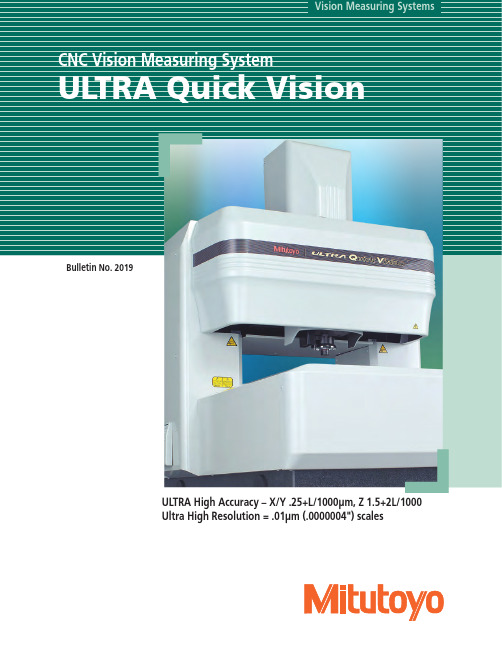
ULTRA High Accuracy – X/Y .25+L/1000µm, Z 1.5+2L/1000 Ultra High Resolution = .01µm (.0000004") scalesThe structural design is optimized through the use of infinite element method (FEM) analysis. This results in maximum rigidity for minimum weight, minimizing deformations due to loading and guaranteeing excellent geometrical accuracy at all times.If a normal air pad is used for the Y axis, it is necessary to increase the mass of the work stage to obtain appropriate rigidity. ULTRA QV (Quick Vision) employs a special air pad called a self-suction type that floats the air pad with compressed air and also generates an absorption power with a vacuum zone provided under negative pressure at the center of the pad. This achieves greater Y-axis rigidity and stage weight reduction concurrently, thus enabling stable stage drive.air temperature on the measuring system structure, the air server supplies air always The thermometer unit installed in the main body reads temperatures at each axis and calculates the amount of expansion and contraction of the body to compensate the measuring accuracy. This function allows the accuracy to be guaranteed in a wide range of 20˚C±2˚C.Additionally, the thermometer unit measures in real time, the workpiece temperatures with two sensors, outputting the results in which dimensions are converted to those at 20˚C.Advanced Technologies Supporting Ultra High-Accuracy SystemsOptimal Structural Design through FEM AnalysisSelf-Suction Air PadTemperature Compensation Function (Option)Conventional glass scaleUltra high-accuracy crystallized glass scaleUltra high-accuracy glass scales are manufactured at the underground laboratory of Mitutoyo Kiyohara Production Department.Compressed airCompressed air Guide planeAir padVacuum suction regionSuctionand in the middle of measuring stroke on a plane using the 5X objective and 1X tube lenstemperature compensation is performed.Those in the case where temperature compensation is*5: An air source is required to maintain the original air pressurebetween 0.5 and 0.9MPa.Unit: Inch (mm)Specifications"Ultra-High Accuracy" Measurement Achieved by Mitutoyo's "ULTRA"Quick VisionThe Ultimate FlagshipMachine NewlyRedesigned withIncreased Speed andHigher AccuracyMitutoyo has NowAttained the Summit ofVision MeasurementOne-Click Point Tool This is a basic tool for capturing one point.One-Click Circle ToolThis tool is appropriate for capturing a full feature circle.One-Click Line ToolThis tool is appropriate for capturing a line feature.One-Click Arc ToolThis tool is appropriate for capturing an arc and theradius of a corner.Pattern SearchT h i s t o o l c a p t u re s t h e position of a pattern that has been registered beforehand. It is optimal for positioningArea Centroid ToolThis tool evaluates the position of a fe a ture's centroid. It is appropriate for capturing the center of a Maximum/Minimum Tool This tool evaluates the maximum or minimum pointwithin the range.Auto Trace ToolThis is a form measuring tool that can autonomously track an unknown feature.The most diverse set of measuring tools available for edge detectionMulti-point auto-focusTargeting the auto-focus tool (surface and pattern) on separate areas allows multiple heights (1344 points at max.) to be measured. Maximum and minimum heights as well as theaverage height can be found.automatically set with one click of the mouse.The removal threshold detection level can be set arbitrarily.Surface Focus Tool This is a general visionfocusing tool.Pattern Focus ToolThis focusing tool is optimal for transparent or low-contrastsurfaces.Edge Focus ToolThis is a tool for focusing on a beveled edge.Noisy edgeNoisy edge Brightness analysisExample of individual layout of focus toolsExample of multiple-height measurement Example of display with the QV graphicsBrightness analysisEdge of Screen Morphological Filterchanges in brightness and differences in texture on the target surface.Advanced edge filtering capabilities including texture, brightness and morphology.alignment, an edge detection error or auto-focus error may result during part program execution.The Smart Recovery function corrects the illumination condition or the position and angle of a tool to automatically perform remeasurement.light intensity correction at procedure creation time, thereby increasing detection repeatability.QV Part ManagerQV Part Manager is the execution program management software for multiple workpieces arranged on the measurement stage.FORMPAK-QV performs contour tolerancing and form analysis from formdata obtained with the QV Auto Trace tool and laser probe.CAD Option displays CAD data on the Graphic window to enhance ease of measurement.A real-time display of measure-mentresults and statistical analysis on the shop floor, with data saved in a database. Includes SPC and statistical analysis, data filtering and reporting systems for complete control of your manu-facturing processes. MeasurLink includes modules for shop floor data collection, QC room data analysis and reporting, gage R&R studies, and gage tracking.QV EioFacilitates external control interface between a PC and QVPAK.QV Eio-PCQVPAK can be controlled from an external PC via RS-232C. QV status can be output using an external I/O board.QV 3DCAD allows the machine to travel to the position specified on a 3DCAD model and execute measurement. This drastically improves the operability and part program creation efficiency compared with operations under joystick control.EASYPAG creates measurement part programs for QVPAK using 2D CAD data. It reduces the number of man-hours for creating part programs, thus allowing a decrease in lead time.PAGPAKPAGPAK is the offline teaching software for creating QVPAK part programs using NC data, CAD data and Gerber data.Pitch circle measurementTool Edit ScreenMeasurement can be performed even if Multiple kinds of workpieces can beQV Eio-PC usage example (System using PATLITE)This hardware allows high-speed focusing or height measurement in a microscopic region with the objective transmission TTL laser.This unit detects temperatures with the main body temperature sensors attached to each axis and two sensors dedicated to a workpiece. The unit finally outputs data converted to dimensions at 20˚C after calculating the expansion and contraction quantities of each main body and workpiece.It is also possible to output dimensions at a reference temperature of 23˚C used in electric and electronics industry although 20˚C is generally assumed as the reference temperature at measurementCalibration Glass ChartThis is a chart for calibration of CCD pixel sizes and offsets between power turrets.Compensation Glass ChartThis is a glass chart of "on-screen compensation" for compensating on-screen distortions an optical system has an "auto-focus compensation" for reducing auto-focus variations resulting from the difference innation or programmable ring light in Quick Vision models that use a hal-ogen light source. This function enhances the visibility of low-reflection surfaces on colored workpieces, facilitating edge detection. This function can also be retrofitted to a conventional Quick Vision. In addition, a yel-low filter enables vision measurement in the yellow light region, which provides high sensitivity.QV-10X, QV-25X: Depending on the workpiece the illumination may be insufficient at aturret lens magnification of 2X and 6X.QV-25X: The PRL illumination is restricted in its usable position.。
python 高密度电法

Python 高密度电法什么是高密度电法高密度电法(High-Density Electrical Resistivity Tomography,简称HDERT)是一种地球物理勘探方法,用于研究地下的电阻率分布。
它通过在地下埋设电极,施加电流并测量电压差,以推断地下的电阻率分布。
高密度电法相比传统的电法方法,具有更高的空间分辨率和更多的数据采集点,可以提供更精细的地下结构信息。
Python 在高密度电法中的应用Python是一种功能强大且广泛应用于科学计算和数据分析的编程语言。
在高密度电法中,Python可以用于数据处理、模型建立、可视化等多个方面。
数据处理高密度电法的数据通常是以文本文件的形式保存的,每个文件包含了多个测点的测量数据。
Python的数据处理库(如NumPy和Pandas)可以帮助我们快速读取、处理和分析这些数据。
以下是一个示例代码,展示了如何使用Python读取和处理高密度电法数据:import numpy as npimport pandas as pd# 读取数据文件data = pd.read_csv('data.csv')# 提取测量数据measurements = data.iloc[:, 1:].values# 计算平均值和标准差mean = np.mean(measurements)std = np.std(measurements)# 打印结果print('平均值:', mean)print('标准差:', std)模型建立在高密度电法中,我们需要建立数学模型来模拟电流在地下的传播和测量。
Python 的科学计算库(如SciPy和scikit-learn)提供了丰富的数值计算和机器学习算法,可以帮助我们构建高密度电法的模型。
以下是一个示例代码,展示了如何使用Python建立高密度电法的模型:from scipy import optimize# 定义模型函数def model_function(x, a, b, c):return a * np.exp(-b * x) + c# 生成样本数据x = np.linspace(0, 10, 100)y = model_function(x, 2, 0.5, 1) + np.random.randn(len(x))# 拟合模型params, params_covariance = optimize.curve_fit(model_function, x, y)# 打印拟合参数print('拟合参数:', params)可视化高密度电法的数据通常是以图像的形式进行展示的,以便更直观地理解地下的电阻率分布。
- 1、下载文档前请自行甄别文档内容的完整性,平台不提供额外的编辑、内容补充、找答案等附加服务。
- 2、"仅部分预览"的文档,不可在线预览部分如存在完整性等问题,可反馈申请退款(可完整预览的文档不适用该条件!)。
- 3、如文档侵犯您的权益,请联系客服反馈,我们会尽快为您处理(人工客服工作时间:9:00-18:30)。
1 High-Radix Floating-Point Division Algorithms for Embedded VLIW Integer Processors(Extended Abstract)Claude-Pierre Jeannerod,Saurabh-Kumar Raina and Arnaud TisserandAr´e naire project(CNRS–ENS Lyon–INRIA–UCBL)LIP,ENS Lyon.46all´e e d’Italie.F–69364LYON Cedex07,FRANCEPhone:+33472728000,Fax:+3372728080E-mail:{fistname}@ens-lyon.frAbstract—This work presentsfloating-point division algo-rithms and implementations for embedded VLIW integer pro-cessors.On those processors,there is no hardwarefloating-point unit,for cost reasons.But,for portability and/or accuracy reasons,a softwarefloating-point emulation layer is sometime useful.In this paper,we focus on high-radix digit-recurrence algorithms forfloating-point division on integer VLIW proces-sors.Our algorithms are targeted for the ST200processor from STMicroelectronics.Index Terms—computer arithmetic,floating-point arithmetic, division,digit-recurrence algorithm,SRT algorithm,high-radix algorithm,integer processor,embedded processor,VLIW proces-sor.I.I NTRODUCTIONThe implementation of fastfloating-point(FP)division is not a trivial task[1],[2].A study from Oberman and Flynn[3] shows that even if the number of issued division instructions is low(around3%for SPEC benchmarks),the total duration of the division computation cannot be neglected(up to40% of the time in arithmetic units).General purpose processors allow fast FP division thanks to a dedicated unit based on the SRT(from the initials of Sweeney,Robertson,and Tocher)algorithm or Newton-Raphson’s algorithm using the FMA(fused multiply and add) of the FP unit(s).Even when a software solution,such as Newton-Raphson’s algorithm,is used,there is some mini-mal hardware support for those algorithms(e.g.,seed tables, see[4].The main division algorithms and implementations used in general purpose processors can be found in a complete survey[5].Most special purpose or embedded processors for digi-tal signal processing,image processing and digital control rely on integer orfixed-point processors,for cost reasons (small area).When implementing algorithms dealing with real numbers on such processors,one has to introduce some scaling operations in the target program,in order to keep accurate computations[6].The insertion of scaling operations is complicated due to the wide range of real numbers required in many applications and it depends on the algorithm and data.Furthermore,scaling is time consuming at both the application and design levels.Of course,algorithms based on FP arithmetic do not have this problem.Then,porting programs from general purpose processors(with FP unit)to integer orfixed-point cores is a complex task.For instance, prototyped applications using Matlab have to be converted to fixed-point format.Furthermore,circuits in these applicationfields seldom integrate dedicated division units.But in order to avoid slow software routines,manufacturers sometimes insert a division step instruction in the ALU(arithmetic and logic unit).Most of the time,this instruction is one step of the non-restoring division algorithm(radix-2).Then a complete n-bit division is done using n steps of this instruction.One goal of this work is to show that some other fast division algorithms may be well suited for the native integer(orfixed-point)hardware support of embedded processors.This work is part of Floating-Point Library for Integer Processor(FLIP).This is a C library for the software support of single precisionfloating-point(FP)arithmetic on processors without FP hardware units such as VLIW or DSP processor cores for embedded applications.Ourfirst target for FLIP is the ST200family of VLIW processors from STMicroelectron-ics(see[7],[8]).Our algorithms can be easily extended to other processors with similar characteristics.In this paper,we focus on pure software division imple-mentation based on high-radix SRT algorithms.We investigate the implementations of these algorithms on processors with rectangular multipliers(e.g.,16×32→32),more or less long latencies for the multiplication unit and parallel functional units(multipliers and ALU).The paper is organized as follows.Section II gives defi-nitions and notations,and recalls the basic algorithms used for software division.Section III presents the SRT algorithm and its extension to high-radix iterations.The implementation on the ST200VLIW processor and its comparison to other solutions are presented in Section IV.In Section V,we briefly present the use of presented algorithms in the case of the FLIP library(Floating-Point Library for Integer Processor).II.B ASIC S OFTWARE D IVISIONDigit-recurrence algorithms produce afixed number of quotient bits at each iteration[9],[1].Such algorithms aresimilar to the “paper-and-pencil”method.The two basic digit-recurrence algorithms are the restoring and the non-restoring algorithms.Those algorithms only rely on very simple radix-2iterations,i.e.one bit of the quotient is produced at each iteration.They are often used in software implementations for low performance applications.Both Newton-Raphson’s and Goldschmidt’s algorithms are based on a functional iteration.The idea is to find an iteration that converges on the quotient value.As an example,Newton-Raphson’s algorithm uses the following functional iteration to evaluate the reciprocal 1/d :y [j +1]=y [j ]×(2−d ×y [j ])where y [j ]is the reciprocal approximation at iteration j .The convergence of this solution is quadratic,that is,the number of correct bits doubles at every iteration.The obtained reciprocal should be multiplied by x in order to complete the computation of the quotient.The initial approximation y 0can be looked up into a table to reduce the number of iterations.This kind of algorithm requires simple arithmetic operators and full-width multiplications (at least in the last iteration).In the following,we will not use this kind of solution because of its long latency for medium precision and because getting a correctly rounded result is much more complicated than using digit-recurrence algorithms.A.Definitions and NotationsIn this paper we follow the definitions and notations pro-posed in [1].The division operation is defined by:x =q ×d +remand|rem |<|d |×ulpandsign (rem )=sign (x )where x is the dividend ,d the divisor ,q the quotient ,and optionally rem the remainder .In our case,we have 0≤x <d and d ∈[1,2).The unit in the last place is ulp =r −n for the radix-r representation of n -digit fractional quotients.In the following,we will use radix-2or radix-2k representations.The value w [j ]denotes the partial remainder obtained at step j .The quotient after j steps is q [j ]= j i =1q i r −i and the final quotient is q =q [n ].B.Restoring AlgorithmThe restoring algorithm uses radix-2quotient digits in the set {0,1}.At each iteration,the algorithm subtracts the divisor d from the partial remainder w (line 4in Figure 1).If the result is strictly less than 0,the previous value should be restored (line 9in Figure 1).Usually,this restoration is not performed using an addition,but by selecting the value 2w [j −1]instead of w [j ],which requires the use of an additional register.1w [0]←−x2f o r j from 1t o n do3w [j ]←−2×w [j −1]4w [j ]←−w [j ]−d 5i f w [j ]≥0then6q j ←−17e l s e8q j ←−09w [j ]←−w [j ]+dFig.1.Restoring division algorithmC.Non-Restoring AlgorithmIn order to avoid the cost of restoration in some cases,the previous algorithm can be modified for radix-2quotient digits in the set {−1,1}instead of {0,1}.The new version,called non-restoring division,presented in Figure 2,allows the same small amount of computations at each iteration.The conversion of the quotient from the digit set {−1,1}to the standard set {0,1}can be done on the fly by using a simple algorithm (see [1]).1w [0]←−x2f o r j from 1t o n do3w [j ]←−2×w [j −1]4i f w [j ]≥0then5w [j ]←−w [j ]−d 6q j ←−17e l s e8w [j ]←−w [j ]+d 9q j ←−−1Fig.2.Non-restoring division algorithmIII.SRT D IVISION A LGORITHMA.Basic AlgorithmThe SRT algorithm,like other digit-recurrence algorithms,is similar to the “paper-and-pencil”method.The main idea in hardware SRT dividers is to use limited comparisons (based on a few most significant bits of d and w [j ])to speed-up quotient selection.Hardware SRT dividers are typically of low complexity,utilize small area,but have relatively large latencies.A complete book is devoted to digit-recurrence algorithms [9]but mainly for hardware implementations.The SRT iteration is based on the computation:w [j +1]←−r ×w [j ]−q j +1×dwhere w [0]=x .At each iteration,the main problem is to determine the new digit of the quotient q j +1.In hardware this is done using a table addressed by a few most significant bits of the divisor d and the partial remainder w [j ].The partial remainder is represented using a redundant notation to speedup the subtraction of q j +1×d from r ×w [j ].In the case of a software implementation,which is our case here,tables for quotient digit selection can not be used(in order to avoid cache misses).Furthermore,a redundant number system is not useful for the partial remainder.B.Standard High-Radix AlgorithmIn our target processors,the rectangle multipliers allow to compute products of one full-width register by one half-width register(i.e.,32×16→32).In a high-radix iteration, this kind of multiplier can be efficiently used to perform the computation q j+1×d.The quotient can be written in a high-radix representation:using radix between28and216for instance.But we need to simplify the new quotient digit selection. The idea of high-radix iterations is to use thefirst most significant bits of the partial remainder as the new quotient digit.To ensure that this trick can be used,the divisor has to be very close to1.This is possible after an initial prescaling step.Prescaling consists here in multiplying both x and d by a value M such that the product M×d is very close to1. The prescaling value is chosen as an approximation of the reciprocal of d(i.e.,M≈1/d).IV.H IGH-R ADIX SRT FOR VLIW I NTEGER P ROCESSOR A.Initial reciprocal approximationWe need M,an initial approximation of the reciprocal such that the value M×d is very close to1.In general purpose processors,one uses a look-up table(such as the Itanium processor[4]).In our case,we will use a polynomial approximation instead. On the interval[1,2](which contains the mantissa of d),the following degree-1polynomial can be used to approximate the function1/d up to4.54bits of accuracy:p(d)=1.457106781−12×dOne has to notice that the4.54bits of accuracy are only the theoretical approximation error.The evaluation error sums up.But for this very specific polynomial,the product1/2×d is performed exactly w.r.t.the internal format.Then,only the subtraction provides an evaluation error(bounded by half an ulp),that is bounded by half a bit.So the total error on the approximation and evaluation on p(d)leads to4bits of accuracy.For this step we compute the following prescaling:M←−p(d)d←−d×Mx←−x×MMultiplying both the numerator and the denominator in the division x/d keep the actual value of the quotient.The only potential problem is to ensure that prescaling can be done without overflow.B.Making d closer to1The previous initial approximation only allows to compute up to4bits at each step of the recurrence.In order to use a higher radix iteration,we want to get a more accurate approx-imation of the reciprocal,i.e.,to make d closer to1.One can use a“better”polynomial approximation.Generally,a more accurate approximation requires a high degree polynomial. Hence,it leads to larger computation time.In our case,we chose to use a part of Goldschmidt’s algorithm.From thefirst approximation,the prescaling step, we have d=1+ .One can easily compute the value1− . Then,the new approximation of the reciprocal is d×(1− )= 1− 2.From a4-bit initial approximation,we now have about 8bits of accuracy for each step.C.High-radix iterationsFrom this starting point,we can now proceed with high-radix SRT iterations.Each iteration gives6bits of the quotient.w[j+1]←−r×w[j]−q j+1×dThe partial remainder w[j]is represented using two’s com-plement representation.It differs from hardware implementa-tions in which w[j]is represented using a redundant number system in order to speedup the subtraction.d is a natural integer.The quotient digit is a small integer on8bits.V.FLIP:F LOATING-P OINT L IBRARY FOR I NTEGERP ROCESSORThis work is a part of FLIP a C library developed in the Ar´e naire team.This library provides thefive basic operations: addition,subtraction,multiplication,division and square-root for a quasi-fully compliant single-precision(SP)IEEE754FP format[10](flags are not supported).This library also provides some running modes with relaxed characteristics:no denormal numbers or restricted rounding modes for instance.This library has been developed and validated within a collaboration with STMicroelectronics.The library has been targeted to the VLIW(very long instruction word)processor cores of the ST200family.Processors of the ST200family executes up to4opera-tions per cycle,with a maximum of one control operation (goto,jump,call,return),one memory operation(load,store, prefetch)and two multiply operations per cycle.All arithmetic instructions operate on integer values,with operands belonging either to the General Registerfile(64×32-bit),or the Branch Registerfile(8×1-bit).The multiply instructions are restricted to16×32-bit on the earlier core variants,but have been recently extended to32-bit by32-bit integer and fractional multiplication on the ST231core.There is no divide instruc-tion but a division step instruction suitable for integer division. In order to reduce the use of conditional branches,the ST200 processor also provides conditional selection instructions.A CKNOWLEDGMENTThis research was supported by the French R´e gion Rhˆo ne-Alpes within the“Arithm´e tique Flottante pour circuits DSP”project.The authors would like to thank Christophe Monat from STMicroelectronics for his valuable support with the ST200environment and Jean-Michel Muller for fruitful dis-cussions.R EFERENCES[1]M.D.Ercegovac and ng,Digital Arithmetic.Morgan Kaufmann,2003.[2]M.J.Flynn and S.F.Oberman,Advanced Computer Arithmetic Design.Wiley-Interscience,2001.[3]S.F.Oberman and M.J.Flynn,“Design issues in division and otherfloating-point operations,”IEEE Transactions on Computers,vol.46, no.2,pp.154–161,Feb.1997.[4]M.Cornea,P.T.P.Tang,and J.Harrison,Scientific Computing onItanium-based Systems.Intel Press,2002.[5]S.Oberman and M.Flynn,“Division algorithms and implementations,”IEEE Transactions on Computers,vol.46,no.8,pp.833–854,Aug.1997.[6] D.Menard and O.Sentieys,“Automatic evaluation of the accuracyoffixed-point algorithms,”in Design,Automation and Test in Europe (DATE),2002,pp.529–537.[7]P.Faraboschi,G.Brown,J.A.Fisher,G.Desoli,and F.Homewood,“Lx:a technology platform for customizable VLIW embedded processing,”in27th Annual International Symposium on Computer Architecture–ISCA’00,June2000.[8]“HP and STMicroelectronics launch”LX”,”/2000/0010/0010feat6.htm.[9]M.D.Ercegovac and ng,Division and Square-Root Algorithms:Digit-Recurrence Algorithms and Implementations.Kluwer Academic, 1994.[10]American National Standards Institute and Institute of Electrical andElectronics Engineers,“IEEE standard for binaryfloating-point arith-metic,”ANSI/IEEE Standard,Std754-1985,1985.。