Non-linear Matrix Factorization with Gaussian Processes

合集下载

非负矩阵分解及其应用探讨

非负矩阵分解及其应用探讨作者：高燕燕来源：《硅谷》2011年第23期摘要：介绍非负矩阵分解（non-negative matrix factorization，NMF）的基本算法思想及其实现过程，并对其在一些重要领域内的应用现状进行概括归纳，最后提出NMF方法在图像处理方面存在的问题及其改进的趋势。

关键词：非负矩阵分解；特征提取；矩阵分解中图分类号：TP391 文献标识码：A 文章编号：1671－7597（2011）1210164－01随着现代计算机处理信息数据的规模越来越大，矩阵作为一种最常见的数据表示形式得到了广泛的应用。

但在实际问题当中，由于矩阵的数据量往往很大，直接处理效率低，意义不大，在实际的操作中，都需要对原始矩阵进行分解。

矩阵分解是将原始矩阵进行适当的分解，使得进一步处理变得简单些。

NMF是D.D.Lee和H.S.Seung在1999年《Nature》中首次提出的算法[1]，该算法要求矩阵中所有元素均为非负的条件下对矩阵进行非负分解。

由于非负矩阵分解实现简单、分解形式和分解结果上的可解释性，以及占用存储空间上的优点，使得非负矩阵分解在实际应用中得到了广泛应用。

1 非负矩阵分解算法1）问题的描述传统NMF问题可描述如下：（1-1）即给定m个n维数据向量集合，每个列向量表示一个样本数据，m为集合中数据样本的个数。

W为基矩阵，H为编码矩阵。

选取的r值一般要求满足，从而可使W和H矩阵的秩远远小于矩阵V的秩。

这样就达到了对原始矩阵V的降维处理。

NMF算法通过“乘性”迭代规则来保证每次迭代后矩阵的元素为非负，保证了非负矩阵分解的可行性。

[2]这种算法实现容易因此得到十分广泛的应用。

2）算法的实现过程NMF算法可以理解为一个带约束的非线性规划的问题，可转化成最优化问题，利用迭代的手段可求解出W和H。

为了求出矩阵分解的结果，Lee和Seung引入了两类目标函数：①矩阵A和B之间的欧氏距离：② Kullback-Leibler散度函数：令A=V，B=WH，可得到用于NMF算法的两类目标函数基于以上两个目标函数，就可得到如下的约束优化问题：和通过合适的迭代规则对以上两个约束优化问题进行收敛得到稳定的矩阵W和H。

奇异值分解与非负矩阵分解的在数据降维方面的特性分析

1.
引言
1999年，《nature》杂志发表了D.D.Lee和H.S.Seung的论文[1]，最早提出了用非负矩阵分解（NMF，Non-negative Matrix Factorization）方法进行大规模数据降维处理的新思想，引起了广大科研人员的密切关注。奇异值分解（SVD，Singular Value Decomposition）是一种较早出现的数据降维与压缩算法。本文将两种不同分解方法进行对比，在Frobenius范数意义下，研究比较两种分解在数据降维的数据量大小、准确性、对不同数据类型的适应能力、矩阵的稀疏性与正交性等方面的特点。
2.
奇异值分解
奇异值分解算法将矩阵X 分解为
X mn U mm mnVnnT
其中U和V是正交矩阵，Σ= Σr 0 0 ，Σr=diag(σ1, σ2,…,σr)，是对角矩阵，其中 0
(1)
r min(m, n, rank ( X )) 。其中σi= λi（i=1,2,…,r）称为矩阵X的奇异值，λ1 ≥λ2 ≥…≥ λr 对应
X1=U1*S1*V1 20 40 60 20 40 60 U1*S2*V1 20 40 60 20 40 60 20 40 60 U1*S2*V3 20 40 60 20 40 60 20 40 60 20 40 60 20 40 60 U1*S1*V3 20 40 60 20 40 60 20 40 60 20 40 60 U2*S4*V2 20 40 60 20 40 60 U1*rand*V1 20 40 60 20 40 60 20 40 620 40 60 U3*S1*V3 20 40 60 20 40 60 U2*rand*V2 U4*S1*V4 X2=U2*S2*V2 20 40 60 20 40 60 U1*S4*V1 X3=U3*S3*V3 20 40 60 20 40 60 X4=U4*S4*V4

Nonnegative Matrix Factorization

Nonnegative Matrix Factorization:A Comprehensive ReviewYu-Xiong Wang,Student Member,IEEE,and Yu-Jin Zhang,Senior Member,IEEE Abstract—Nonnegative Matrix Factorization(NMF),a relatively novel paradigm for dimensionality reduction,has been in the ascendant since its inception.It incorporates the nonnegativity constraint and thus obtains the parts-based representation as well as enhancing the interpretability of the issue correspondingly.This survey paper mainly focuses on the theoretical research into NMF over the last5years,where the principles,basic models,properties,and algorithms of NMF along with its various modifications,extensions, and generalizations are summarized systematically.The existing NMF algorithms are divided into four categories:Basic NMF(BNMF), Constrained NMF(CNMF),Structured NMF(SNMF),and Generalized NMF(GNMF),upon which the design principles,characteristics,problems,relationships,and evolution of these algorithms are presented and analyzed comprehensively.Some related work not on NMF that NMF should learn from or has connections with is involved too.Moreover,some open issues remained to be solved are discussed.Several relevant application areas of NMF are also briefly described.This survey aims to construct an integrated,state-of-the-art framework for NMF concept,from which the follow-up research may benefit.Index Terms—Data mining,dimensionality reduction,multivariate data analysis,nonnegative matrix factorization(NMF)Ç1I NTRODUCTIONO NE of the basic concepts deeply rooted in science and engineering is that there must be something simple, compact,and elegant playing the fundamental roles under the apparent chaos and complexity.This is also the case in signal processing,data analysis,data mining,pattern recognition,and machine learning.With the increasing quantities of available raw data due to the development in sensor and computer technology,how to obtain such an effective way of representation by appropriate dimension-ality reduction technique has become important,necessary, and challenging in multivariate data analysis.Generally speaking,two basic properties are supposed to be satisfied: first,the dimension of the original data should be reduced; second,the principal components,hidden concepts,promi-nent features,or latent variables of the data,depending on the application context,should be identified efficaciously.In many cases,the primitive data sets or observations are organized as data matrices(or tensors),and described by linear(or multilinear)combination models;whereupon the formulation of dimensionality reduction can be regarded as, from the algebraic perspective,decomposing the original data matrix into two factor matrices.The canonical methods, such as Principal Component Analysis(PCA),Linear Discriminant Analysis(LDA),Independent Component Analysis(ICA),Vector Quantization(VQ),etc.,are the exemplars of such low-rank approximations.They differ from one another in the statistical properties attributable to the different constraints imposed on the component matrices and their underlying structures;however,they have something in common that there is no constraint in the sign of the elements in the factorized matrices.In other words,the negative component or the subtractive combina-tion is allowed in the representation.By contrast,a new paradigm of factorization—Nonnegative Matrix Factoriza-tion(NMF),which incorporates the nonnegativity constraint and thus obtains the parts-based representation as well as enhancing the interpretability of the issue correspondingly, was initiated by Paatero and Tapper[1],[2]together with Lee and Seung[3],[4].As a matter of fact,the notion of NMF has a long history under the name“self modeling curve resolution”in chemometrics,where the vectors are continuous curves rather than discrete vectors[5].NMF was first introduced by Paatero and Tapper as the concept of Positive Matrix Factorization,which concentrated on a specific application with Byzantine algorithms.These shortcomings limit both the theoretical analysis,such as the convergence of the algorithms or the properties of the solutions,and the generalization of the algorithms in other applications. Fortunately,NMF was popularized by Lee and Seung due to their contributing work of a simple yet effective algorithmic procedure,and more importantly the emphasis on its potential value of parts-based representation.Far beyond a mathematical exploration,the philosophy underlying NMF,which tries to formulate a feasible model for learning object parts,is closely relevant to perception mechanism.While the parts-based representation seems intuitive,it is indeed on the basis of physiological and psychological evidence:perception of the whole is based on perception of its parts[6],one of the core concepts in certain computational theories of recognition problems.In fact there are two complementary connotations in nonnegativity—nonnegative component and purely additive combination. On the one hand,the negative values of both observations.The authors are with the Tsinghua National Laboratory for InformationScience and Technology and the Department of Electronic Engineering,Tsinghua University,Rohm Building,Beijing100084,China.E-mail:albertwyx@,zhang-yj@.Manuscript received21July2011;revised2Nov.2011;accepted4Feb.2012;published online2Mar.2012.Recommended for acceptance by L.Chen.For information on obtaining reprints of this article,please send e-mail to:tkde@,and reference IEEECS Log Number TKDE-2011-07-0429.Digital Object Identifier no.10.1109/TKDE.2012.51.1041-4347/13/$31.00ß2013IEEE Published by the IEEE Computer Societyand latent components are physically meaningless in many kinds of real-world data,such as image,spectra,and gene data,analysis tasks.Meanwhile,the discovered prototypes commonly correspond with certain semantic interpretation. For instance,in face recognition,the learned basis images are localized rather than holistic,resembling parts of faces,such as eyes,nose,mouth,and cheeks[3].On the other hand, objects of interest are most naturally characterized by the inventory of its parts,and the exclusively additive combina-tion means that they can be reassembled by adding required parts together similar to identikits.NMF thereupon has achieved great success in real-word scenarios and tasks.In document clustering,NMF surpasses the classic methods, such as spectral clustering,not only in accuracy improve-ment but also in latent semantic topic identification[7].To boot,the nonnegativity constraint will lead to sort of sparseness naturally[3],which is proved to be a highly effective representation distinguished from both the com-pletely distributed and the solely active component de-scription[8].When NMF is interpreted as a neural network learning algorithm depicting how the visible variables are generated from the hidden ones,the parts-based represen-tation is obtained from the additive model.A positive number indicates the presence and a zero value represents the absence of some event or component.This conforms nicely to the dualistic properties of neural activity and synaptic strengths in neurophysiology:either excitatory or inhibitory without changing sign[3].Because of the enhanced semantic interpretability under the nonnegativity and the ensuing sparsity,NMF has become an imperative tool in multivariate data analysis, and been widely used in the fields of mathematics, optimization,neural computing,pattern recognition and machine learning[9],data mining[10],signal processing [11],image engineering and computer vision[11],spectral data analysis[12],bioinformatics[13],chemometrics[1], geophysics[14],finance and economics[15].More specifi-cally,such applications include text data mining[16],digital watermark,image denoising[17],image restoration,image segmentation[18],image fusion,image classification[19], image retrieval,face hallucination,face recognition[20], facial expression recognition[21],audio pattern separation [22],music genre classification[23],speech recognition, microarray analysis,blind source separation[24],spectro-scopy[25],gene expression classification[26],cell analysis, EEG signal processing[17],pathologic diagnosis,email surveillance[10],online discussion participation prediction, network security,automatic personalized summarization, identification of compounds in atmosphere analysis[14], earthquake prediction,stock market pricing[15],and so on.There have been numerous results devoted to NMF research since its inception.Researchers from various fields, mathematicians,statisticians,computer scientists,biolo-gists,and neuroscientists,have explored the NMF concept from diverse perspectives.So a systematic survey is of necessity and consequence.Although there have been such survey papers as[27],[28],[12],[13],[10],[11],[29]and one book[9],they fail to reflect either the updated or the comprehensive results.This review paper will summarize the principles,basic models,properties,and algorithms of NMF systematically over the last5years,including its various modifications,extensions,and generalizations.A taxonomy is accordingly proposed to logically group them, which have not been presented before.Besides these,some related work not on NMF that NMF should learn from or has connections with will also be involved.Furthermore, this survey mainly focuses on the theoretical research rather than the specific applications,the practical usage will also be concerned though.It aims to construct an integrated, state-of-the-art framework for NMF concept,from which the follow-up research may benefit.In conclusion,the theory of NMF has advanced sig-nificantly by now yet is still a work in progress.To be specific:1)the properties of NMF itself have been explored more deeply;whereas a firm statistical underpinning like those of the traditional factorization methods—PCA or LDA—is not developed fully(partly due to its knottiness).2)Some problems like the ones mentioned in[29]have been solved,especially those with additional constraints;never-theless a lot of other questions are still left open.The existing NMF algorithms are divided into four categories here given in Fig.1,following some unified criteria:1.Basic NMF(BNMF),which only imposes the non-negativity constraint.2.Constrained NMF(CNMF),which imposes someadditional constraints as regularization.3.Structured NMF(SNMF),which modifies the stan-dard factorization formulations.4.Generalized NMF(GNMF),which breaks throughthe conventional data types or factorization modesin a broad sense.The model level from Basic to Generalized NMF becomes broader.Therein Basic NMF formulates the fundamental analytical framework upon which all other NMF models are built.We will present the optimization tools and computational methods to efficiently and robustly solve Basic NMF.Moreover,the pragmatic issue of NMF with respect to large-scale data sets and online processing will also be discussed.Constrained NMF is categorized into four subclasses:1.Sparse NMF(SPNMF),which imposes the sparse-ness constraint.2.Orthogonal NMF(ONMF),which imposes theorthogonality constraint.3.Discriminant NMF(DNMF),which involves theinformation for classification and discrimination.4.NMF on manifold(MNMF),which preserves thelocal topological properties.We will demonstrate why these morphological constraints are essentially necessary and how to incorporate them into the existing solution framework of Basic NMF.Correspondingly,Structured NMF is categorized into three subclasses:1.Weighed NMF(WNMF),which attaches differentweights to different elements regarding their relativeimportance.2.Convolutive NMF (CVNMF),which considers the time-frequency domain factorization.3.Nonnegative Matrix Trifactorization (NMTF),whichdecomposes the data matrix into three factor matrices.Besides,Generalized NMF is categorized into four subclasses:1.Semi-NMF,which relaxes the nonnegativity con-straint only on the specific factor matrix.2.Nonnegative Tensor Factorization (NTF),whichgeneralizes the matrix-form data to higher dimen-sional tensors.3.Nonnegative Matrix-Set Factorization (NMSF),which extends the data sets from matrices to matrix-sets.4.Kernel NMF (KNMF),which is the nonlinear modelof NMF.The remainder of this paper is organized as follows:first,the mathematic formulation of NMF model is presented,and the unearthed properties of NMF are summarized.Then the algorithmic details of foregoing categories of NMF are elaborated.Finally,conclusions are drawn,and some open issues remained to be solved are discussed.2C ONCEPT AND P ROPERTIES OF NMFDefinition.Given an M dimensional random vector x with nonnegative elements,whose N observations are denoted asx j;j ¼1;2;...;N ,let data matrix be X ¼½x 1;x 2;...;x N 2I R M ÂN!0,NMF seeks to decompose X into nonnegative M ÂL basismatrix U ¼½u 1;u 2;...;u L 2I R M ÂL!0and nonnegative L ÂN coefficient matrix V ¼½v 1;v 2;...;v N 2I R L ÂN!0,such thatX %U V ,where I R M ÂN!0stands for the set of M ÂN element-wise nonnegative matrices.This can also be written as the equivalent vector formula x j %P Li ¼1u i V ij .It is obvious that v j is the weight coefficient of the observation x j on the columns of U ,the basis vectors or the latent feature vectors of X .Hence,NMF decomposes each data into the linear combination of the basis vectors.Because of the initial condition L (min ðM;N Þ,the obtained basis vectors are incomplete over the original vector space.In other words,this approach tries to represent the high-dimensional stochastic pattern with far fewer bases,so the perfect approximation can be achieved successfully only if the intrinsic features are identified in U .Here,we discuss the relationship between L and M ,N a little more.In most cases,NMF is viewed as a dimension-ality reduction and feature extraction technique with L (M;L (N ;that is,the basis set learned from NMF model is incomplete,and the energy is compacted.However,in general,L can be smaller,equal or larger than M .But there are fundamental differences in the decomposition for L <M and L >M .It is a sort of sparse coding and compressed sensing with overcomplete basis when L >M .Hence,L need not be limited by the dimensionality of the data,which is useful for some applications,like classification.In this situation,it may benefit from the sparseness due to both nonnegativity and redundant representation.One approach to obtain this NMF model is to perform the decomposition on the residue matrix E ¼X ÀU V repeat-edly and sequentially [30].As a kind of matrix factorization model,three essential questions need answering:1)existence,whether the nontrivial NMF solutions exist;2)uniqueness,under what assumptions NMF is,at least in some sense,unique;3)effectiveness,under what assumptions NMF is able to recover the “right answer.”The existence was showed via the theory of Completely Positive (CP)Factorization for the first time in [31].The last two concerns were first mentioned and discussed from a geometric viewpoint in [32].Complete NMF X ¼U V is considered first for the analysis of existence,convexity,and computational com-plexity.The trivial solution always exists as U ¼X and V ¼I N .By relating NMF to CP Factorization,Vasiloglou et al.showed that every nonnegative matrix has a nontrivial complete NMF [31].As such,CP Factorizationis a special case,where a nonnegative matrix X 2I R M ÂM!0is CP if it can be factored in the form X ¼U U T ;U 2I R M ÂL!0.The minimum L is called the CP-rank of X .WhenFig.1.The categorization of NMF models and algorithms.combining that the set of CP matrices forms a convex cone with that the solution to NMF belongs to a CP cone, solving NMF is a convex optimization problem[31]. Nevertheless,finding a practical description of the CP cone is still open,and it remains hard to formulate NMF as a convex optimization problem,despite a convex relaxation to rank reduction with theoretical merit pro-posed in[31].Using the bilinear model,complete NMF can be rewritten as linear combination of rank-one nonnegative matrices expressed byX¼X Li¼1U i V i ¼X Li¼1U i V iðÞT;ð1Þwhere U i is the i th column vector of U while V i is the i th row vector of V,and denotes the outer product of two vectors.The smallest L making the decomposition possible is called the nonnegative rank of the nonnegative matrix X, denoted as rankþðXÞ.And it satisfies the following trivial bounds[33]rankðXÞrankþðXÞminðM;NÞ:ð2ÞWhile PCA can be solved in polynomial time,the optimization problem of NMF,with respect to determining the nonnegative rank and computing the associated factor-ization,is more difficult than its unconstrained counterpart. It is in fact NP-hard when requiring both the dimension and the factorization rank of X to increase,which was proved via relating it to NP-hard intermediate simplex problem by Vavasis[34].This is also the corollary of CP programming, since the CP cone cannot be described in polynomial time despite its convexity.In the special case when rankðXÞ¼1, complete NMF can be solved in polynomial time.However, the complexity of complete NMF for fixed factorization rank generally is still unknown[35].Another related work is so-called Nonnegative Rank Factorization(NRF)focusing on the situation of rankðXÞ¼rankþðXÞ,i.e.,selecting rankðXÞas the minimum L[33]. This is not always possible,and only nonnegative matrix with a corresponding simplicial cone(A polyhedral cone is simplicial if its vertex rays are linearly independent.) existed has an NRF[36].In most cases,the approximation version of NMF X% U V instead of the complete factorization is widely utilized. An alternative generative model isX¼U VþE;ð3Þwhere E2I R MÂN is the residue or noise matrix represent-ing the approximation error.These two modes of NMF are essentially coupled with each other,though much more attention is devoted to the latter.The theoretical results on complete NMF will be helpful to design more efficient NMF algorithms[31],[34]. The selection of the factorization rank L of NMF may be more creditable if tighter bound for the nonnegative rank is obtained[37].In essence,NMF is an ill-posed problem with nonunique solutions[32],[38].From the geometric perspective,NMF can be viewed as finding a simplicial cone involving all the data points in the positive orthant.Given a simplicial cone satisfying all these conditions,it is not difficult to construct another cone containing the former one to meet the same conditions,so the nesting can work on infinitively thus leading to an ill-defined factorization notion.From the algebraic perspective,if there exists a solution X%U0V0, let U¼U0D,V¼DÀ1V0,then X%U V.If a nonsingular matrix and its inverse are both nonnegative,then the matrix is a generalized permutation with the form of P S, where P and S are permutation and scaling matrices, respectively.So the permutation and scaling ambiguities for NMF are inevitable.For that matter,NMF is called unique factorization up to a permutation and a scaling transformation when D¼P S.Unfortunately,there are many ways to select a rotational matrix D which is not necessarily a generalized permutation or even nonnegative matrix,so that the transformed factor matrices U and V are still nonnegative.In other words,the sole nonnegativity constraint in itself will not suffice to guarantee the uniqueness,let alone the effectiveness.Nevertheless,the uniqueness will be achieved if the original data satisfy certain generative model.Intuitively,if U0and V0are sufficiently sparse,only generalized permutation matrices are possible rotation matrices satisfying the nonnegativity constraint.Strictly speaking,this is called boundary close condition for sufficiency and necessity of the uniqueness of NMF solution[39].The deep discussions about this issue can be found in[32],[38],[39],[40],[41],and[42].In practice,incorporating additional constraints such as sparseness in the factor matrices or normalizing the columns of U(respectively rows of V)to unit length is helpful in alleviating the rotational indeterminacy[9].It was hoped that NMF would produce an intrinsically parts-based and sparse representation in unsupervised mode[3],which is the most inspiring benefit of NMF. Intuitively,this can be explained by that the stationary points of NMF solutions will typically be located at the boundary of the feasible domain due to the first order optimality conditions,leading to zero elements[37].Further experiments by Li et al.have shown,however,that the pure additivity does not necessarily mean sparsity and that NMF will not necessarily learn the localized features[43].Further more,NMF is equivalent to k-means clustering when using Square of Euclidian Distance(SED)[44],[45], while tantamount to Probabilistic Latent Semantic Analy-sis(PLSA)when using Generalized Kullback-Leibler Divergence(GKLD)as the objective function[46],[47].So far we may conclude that the merits of NMF,parts-based representation and sparseness included,come at the price of more complexity.Besides,SVD or PCA has always a more compact spectrum than NMF[31].You just cannot have the best of both worlds.3B ASIC NMF A LGORITHMSThe cynosure in Basic NMF is trying to find more efficient and effective solutions to NMF problem under the sole nonnegativity constraint,which lays the foundation for the practicability of NMF.Due to its NP-hardness and lack of appropriate convex formulations,the nonconvex formula-tions with relatively easy solvability are generally adopted,and only local minima are achievable in a reasonable computational time.Hence,the classic and also more practical approach is to perform alternating minimization of a suitable cost function as the similarity measures between X and the product U V .The different optimization models vary from one another mainly in the object functions and the optimization procedures.These optimization models,even serving to give sight of some possible directions for the solutions to Constrained,Structured,and Generalized NMF,are the kernel discus-sions of this section.We will first summarize the objective functions.Then the details about the classic Basic NMF framework and the paragon algorithms are presented.Moreover,some new vision of NMF,such as the geometric formulation of NMF,and the pragmatic issue of NMF,such as large-scale data sets,online processing,parallel comput-ing,and incremental NMF,will be discussed.In the last part of this section,some other relevant issues are also involved.3.1Similarity Measures or Objective FunctionsIn order to quantify the difference between the original data X and the approximation U V ,a similarity measure D ðX U V k Þneeds to be defined first.This is also the objective function of the optimization model.These similarity mea-sures can be either distances or divergences,and correspond-ing objective functions can be either a sole cost function or optionally a set of cost functions with the same global minima to be minimized sequentially or simultaneously.The most commonly used objective functions are SED (i.e.,Frobenius norm)(4)and GKLD (i.e.,I-divergence)(5)[4]D F X U V k ðÞ¼12X ÀU V k k 2F ¼12X ijX ij ÀU V ½ ij 2;ð4ÞD KL X U V k ðÞ¼XijX ij lnX ijU V ½ ijÀX ij þU V ½ ij !:ð5ÞThere are some drawbacks of GKLD,especially the gradients needed in optimization heavily depend on the scales of factorizing matrices leading to many iterations.Thus,the original KLD is renewed for NMF by normalizing the input data in [48].Other cost functions consist of Minkowski family of metrics known as ‘p -norm,Earth Mover’s distance metric [18], -divergence [17], -divergence [49], -divergence [50],Csisza´r’s ’-divergence [51],Bregman divergence [52],and - -divergence [53].Most of them are element-wise mea-sures.Some similarity measures are more robust with respect to noise and outliers,such as hypersurface cost function [54], -divergence [50],and - -divergence [53].Statistically,different similarity measures can be deter-mined based on a prior knowledge about the probability distribution of the noise,which actually reflects the statistical structure of the signals and the disclosed compo-nents.For example,the SED minimization can be seen as a maximum likelihood estimator where the difference is due to additive Gaussian noise,whereas GKLD can be shown to be equivalent to the Expectation Maximization (EM)algo-rithm and maximum likelihood for Poisson processes [9].Given that while the optimization problem is not jointly convex in both U and V ,it is separately convex in either Uor V ,the alternating minimizations are seemly the feasible direction.A phenomenon worthy of notice is that although the generative model of NMF is linear,the inference computation is nonlinear.3.2Classic Basic NMF Optimization Framework The prototypical multiplicative update rules originated by Lee and Seung—the SED-MU and GKLD-MU [4]have still been widely used as the baseline.The SED-MU and GKLD-MU algorithms use SED and GKLD as objective functions,respectively,and both apply iterative multiplicative updates as the optimization approach similar to EM algorithms.In essence,they can be viewed as adaptive rescaled gradient descent algorithms.Considering the efficiency,they are relatively simple and parameter free with low cost per iteration,but they converge slowly due to a first-order convergence rate [28],[55].Regarding the quality of the solutions,Lee and Seung claimed that the multiplicative update rules converge to a local minimum [4].Gonzales and Zhang indicated that the gradient and properties of continual nonincreasing by no means,however,ensure the convergence to a limit point that is also a stationary point,which can be understood under the Karush-Kuhn-Tucker (KKT)optimality conditions [55],[56].So the accurate conclusion is that the algorithms converge to a stationary point which is not necessarily a local minimum when the limit point is in the interior of the feasible region;its stationarity cannot be even determined when the limit point lies on the boundary of the feasible region [10].However,a minor modification in their step size of the gradient descent formula achieves a first-order stationary point [57].Another drawback is the strong correlation enforced by the multi-plication.Once an element in the factor matrices becomes zero,it must remain zero.This means the gradual shrinkage of the feasible region,which is harmful for getting more superior solution.In practice,to reduce the numerical difficulties,like numerical instabilities or ill-conditioning,the normalization of the ‘1or ‘2norm of the columns in U is often needed as an extra procedure,yet this simple trick has changed the original optimization problem,thereby making searching for the global minimum more complicated.Besides,to preclude the computational difficulty due to division by zero,an extra positive additive value in the denominator is helpful [56].To accelerate the convergence rate,one popular method is to apply gradient descent algorithms with additive update rules.Other techniques such as conjugate gradient,projected gradient,and more sophisticated second-order scheme like Newton and Quasi-Newton methods et al.are also in consideration.They choose appropriate descent direction,such as the gradient direction,and update the element additively in the factor matrices at a certain learning rate.They differ from one another as for either the descent direction or the learning rate strategy.To satisfy the nonnegativity constraint,the updated matrices are brought back to the feasible region,namely the nonnegative orthant,by additional projection,like simply setting all negative elements to ually under certain mild additional conditions,they can guarantee the first-order stationarity.These are the widely developed algorithms in Basic NMF recent years.。

Projected gradient methods for non-negative matrix factorization

1
Introduction
Non-negative matrix factorization (NMF) (Paatero and Tapper, 1994; Lee and Seung, 1999) is useful for ﬁnding representations of non-negative data. Given an n × m data matrix V with Vij ≥ 0 and a pre-speciﬁed positive integer r < min(n, m), NMF ﬁnds two non-negative matrices W ∈ Rn×r and H ∈ Rr×m such that V ≈ W H. If each column of V represents an object, NMF approximates it by a linear combination of r “basis” columns in W . NMF has been applied to many areas such as ﬁnding basis vectors of images (Lee and Seung, 1999), document clustering (Xu et al., 2003), molecular pattern discovery (Brunet et al., 2004), etc. Donoho and 1
Stodden (2004) have addressed the theoretical issues associated with the NMF approach. The conventional approach to ﬁnd W and H is by minimizing the diﬀerence between V and W H : min

非负矩阵分解模型算法和应用

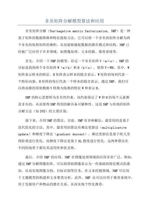
非负矩阵分解模型算法和应用非负矩阵分解（Non-negative matrix factorization, NMF）是一种基于矩阵的数据降维和特征提取方法，它可以将一个非负的矩阵分解为两个非负的低秩矩阵的乘积，从而能够捕捉数据的潜在模式和结构。

NMF已经被广泛应用于许多领域，如图像处理、文本挖掘、推荐系统等。

首先，介绍一下NMF的模型。

给定一个非负矩阵V（m×n），NMF的目标是找到两个非负矩阵W（m×k）和H（k×n），使得V≈WH。

其中，W矩阵表示样本的特征，H矩阵表示样本的隐含表示。

W矩阵的每列代表一个特征向量，H矩阵的每行代表一个样本的隐含表示。

通过NMF，我们可以将高维的原始数据V转换为低维的特征W和表示H。

NMF的核心思想即为非负性约束。

该约束保证了W和H的每个元素都是非负的，从而使得NMF得到的解具备可解释性。

这是NMF与传统的矩阵分解方法（如SVD）的主要区别。

接下来，介绍NMF的算法。

目前，NMF有多种解法，最常用的是基于迭代优化的方法。

其中，最常用的算法有乘法更新法（multiplicative update）和梯度下降法（gradient descent）。

乘法更新法是基于欧几里得距离进行优化，而梯度下降法是基于KL散度进行优化。

这两种算法在不同的场景下都有其适用性和优劣势。

最后，介绍NMF的应用。

NMF在图像处理领域的应用非常广泛。

例如，通过NMF分解图像矩阵，可以将原始图像表示为一些基础的特征模式的叠加，从而实现图像分割、目标识别等任务。

在文本挖掘领域，NMF可以用于主题模型的构建和文本聚类分析。

此外，NMF还可以应用于推荐系统中，用于发掘用户和物品的潜在关系，从而实现个性化推荐。

总结来说，非负矩阵分解是一种非常有用的数据降维和特征提取方法。

它通过将原始数据矩阵分解为非负的低秩矩阵的乘积，可以捕捉到数据的潜在模式和结构。

NMF已经被广泛应用于图像处理、文本挖掘、推荐系统等领域，为这些领域的发展和进步做出了重要贡献。

Graph Regularized Nonnegative Matrix

Ç
1 INTRODUCTION
HE
techniques for matrix factorization have become popular in recent years for data representation. In many problems in information retrieval, computer vision, and pattern recognition, the input data matrix is of very high dimension. This makes learning from example infeasible [15]. One then hopes to find two or more lower dimensional matrices whose product provides a good approximation to the original one. The canonical matrix factorization techniques include LU decomposition, QR decomposition, vector quantization, and Singular Value Decomposition (SVD). SVD is one of the most frequently used matrix factorization techniques. A singular value decomposition of an M Â N matrix X has the following form: X ¼ UÆVT ; where U is an M Â M orthogonal matrix, V is an N Â N orthogonal matrix, and Æ is an M Â N diagonal matrix with Æij ¼ 0 if i 6¼ j and Æii ! 0. The quantities Æii are called the singular values of X, and the columns of U and V are called

属于映射数据到新的空间的方法

属于映射数据到新的空间的方法映射数据到新的空间是一种常见的数据处理方法，它可以将原始数据转换为具有新特征的数据，以便更好地理解和分析。

在本文中，将介绍几种常用的方法来实现数据映射，包括主成分分析、流形学习和自编码器。

一、主成分分析（Principal Component Analysis，PCA）主成分分析是一种常用的线性降维方法，它通过线性变换将原始数据映射到一个新的空间，使得新空间中的样本具有最大的方差。

主成分分析的核心思想是将原始数据在协方差矩阵的特征向量方向上进行投影，从而得到新的特征向量。

这些特征向量被称为主成分，它们按照对应的特征值大小排序，表示数据中的主要变化方向。

通过选择前几个主成分，可以实现数据的降维，同时保留较多的信息。

二、流形学习（Manifold Learning）流形学习是一种非线性降维方法，它假设高维数据分布在一个低维流形上，并试图通过学习这个流形的结构来实现数据的映射。

流形学习方法可以保留原始数据的局部结构和全局结构，能够更好地处理非线性数据。

常用的流形学习方法包括等度量映射（Isomap）、局部线性嵌入（Locally Linear Embedding，LLE）和拉普拉斯特征映射（Laplacian Eigenmaps）等。

这些方法通过计算样本之间的距离或相似度来构建流形结构，并将原始数据映射到低维空间中。

三、自编码器（Autoencoder）自编码器是一种无监督学习的神经网络模型，它可以将输入数据压缩成一个低维的编码表示，并尽可能地通过解码器将编码后的数据重构为原始输入。

自编码器的目标是最小化重构误差，从而学习到数据的有效表示。

自编码器有多种变体，包括稀疏自编码器、去噪自编码器和变分自编码器等。

自编码器可以在无标签数据上进行训练，因此适用于无监督的数据映射任务。

除了上述方法，还有一些其他的数据映射方法，如非负矩阵分解（Non-negative Matrix Factorization，NMF）、线性判别分析（Linear Discriminant Analysis，LDA）和高斯过程回归（Gaussian Process Regression，GPR）等。

Nonnegative matrix factorization and applications

NONNEGATIVE MATRIX F ACTORIZATION AND APPLICATIONSMOODY CHU and ROBERT PLEMMONSDepartment of Mathematics,North Carolina State University,Raleigh,NC27695-8205. Departments of Computer Science and Mathematics,Wake Forest University,Winston-Salem,NC27109. 1IntroductionData analysis is pervasive throughout science,engineering and business applications.Very often the data to be analyzed is nonnegative,and it is very often preferable to take this constraint into account in the analysis process.In this paper we provide a survey of some aspects of nonnegative matrix factorization and its applications to nonnegative matrix data analysis.In general the problem is the following:given a nonnegative data matrix Yﬁnd reduced rank nonnegative matrices U and V so thatY≈UV.Here,U is often thought of as the source matrix and V as the mixing matrix associated with the data in Y.A more formal deﬁnition of the problem is given below.This approximate factorization process is an active area of research in several disciplines(a Google search on this topic recently provided over250references to papers involving nonnegative matrix factorization and applications written in the past ten years),and the subject is certainly a fertile area of research for linear algebraists.An indispensable task in almost every discipline is to analyze a certain data to search for relationships between a set of exogenous and endogenous variables.There are two special concerns in data analysis.First, most of the information gathering devices or methods at present have onlyﬁnite bandwidth.One thus cannot avoid the fact that the data collected often are not exact.For example,signals received by antenna arrays often are contaminated by instrumental noises;astronomical images acquired by telescopes often are blurred by atmospheric turbulence;database prepared by document indexing often are biased by subjective judgment; and even empirical data obtained in laboratories often do not satisfy intrinsic physical constraints.Before any deductive sciences can further be applied,it is important toﬁrst reconstruct or represent the data so that the inexactness is reduced while certain feasibility conditions are satisﬁed.Secondly,in many situations the data observed from complex phenomena represent the integrated result of several interrelated variables acting together.When these variables are less precisely deﬁned,the actual information contained in the original data might be overlapping and ambiguous.A reduced system model could provide aﬁdelity near the level of the original system.One common ground in the various approaches for noise removal,model reduction,feasibility reconstruction,and so on,is to replace the original data by a lower dimensional representation obtained via subspace approximation.The notion of low rank approximations therefore arises in a wide range of important applications.Factor analysis and principal component analysis are two of the many classical methods used to accomplish the goal of reducing the number of variables and detecting structures among the variables.However,as indicated above,often the data to be analyzed is nonnegative,and the low rank data are further required to be comprised of nonnegative values only in order to avoid contradicting physical realities. Classical tools cannot guarantee to maintain the nonnegativity.The approach of low-rank nonnegative matrix factorization(NNMF)thus becomes particularly appealing.The NNMF problem,probably due originally to Paatero and Tapper[21],can be stated in generic form as follows:(NNMF)Given a nonnegative matrix Y∈R m×n and a positive integer p<min{m,n},ﬁnd nonnegative matrices U∈R m×p and V∈R p×n so as to minimize the functionalf(U,V):=12Y−UV 2F.(1)The product UV of the least squares solution is called a nonnegative matrix factorization of Y,although Y is not necessarily equal to the product UV.Clearly the product UV is of rank at most p.An appropriate decision on the value of p is critical in practice,but the choice of p is very often problem dependent.The objective function(1)can be modiﬁed in several ways to reﬂect the application need.For example,penalty1terms can be added to f(U,V)in order to enforce sparsity or to enhance smoothness in the solution U and V[13,24].Also,because UV=(UD)(D−1V)for any invertible matrix D∈R p×p,sometimes it is desirable to“normalize”columns of U The question of uniqueness of the nonnegative factors U and V also arises, which is easily seen by considering case where the matrices D and D−1are nonnegative.For simplicity, we shall concentrate on(1)only in this essay,but the metric to be minimized in the NNMF problem can certainly be generalized and constraints beyond nonnegativity are sometimes imposed for speciﬁc situations, e.g.,[5,13,14,15,18,19,24,25,26,27].In many applications,we will see that the p factors,interpreted as either sources,basis elements,or concepts,play a vital role in data analysis.In practice,there is a need to determine as few factors as possible and,hence the need for a low rank NNMF of the data matrix Y arises. 2Some ApplicationsThe basic idea behind the NNMF is the linear model.The matrix Y=[y ij]∈R m×n in the NNMF formulation denotes the“observed”data whereas each entry y ij represents,in a broad sense,the score obtained by entity j on variable i.One way to characterize the interrelationships among multiple variables that contribute to the observed data Y is to assume that y ij is a linearly weighted score by entity j based on several“factors”. We shall temporarily assume that there are p factors,but often it is precisely the point that the factors are to be retrieved in the mining process.A linear model,therefore,assumes the relationshipY=AF,(2) where A=[a ik]∈R m×p is a matrix with a ik denoting the loading of variable i to factor k or,equivalently, the inﬂuence of factor k on variable i,and F=[f kj]∈R p×n with f kj denoting the score on factor k by entity j or the response of entity j to factor k.Depending on the applications,there are many ways to interpret the meaning of the linear model.We brieﬂy describe a few applications below.2.1Air Emission QualityIn the air pollution research community,one observational technique makes use of the ambient data and source proﬁle data to apportion sources or source categories[12,15].The fundamental principle in this model is that mass conservation can be assumed and a mass balance analysis can be used to identify and apportion sources of airborne particulate matter in the atmosphere.For example,it might be desirable to determine a large number of chemical constituents such as elemental concentrations in a number of samples.The relationships between p sources which contribute m chemical species to n samples,therefore,lead to a mass balance equation,y ij=pk=1a ik f kj,(3)where y ij is the elemental concentration of the i th chemical measured in the j th sample,a ik is the gravimetric concentration of the i th chemical in the k th source,and f kj is the airborne mass concentration that the k th source has contributed to the j th sample.In a typical scenario,only values of y ij are observable whereas neither the sources are known nor the compositions of the local particulate emissions are measured.Thus,a critical question is to estimate the number p,the compositions a ik,and the contributions f kj of the sources.Tools that have been employed to analyze the linear model include principal component analysis,factor analysis,cluster analysis,and other multivariate statistical techniques.In this receptor model,however,there is a physical constraint imposed upon the data.That is,the source compositions a ik and the source contributions f kj must all be nonnegative.The identiﬁcation and apportionment,therefore,becomes a nonnegative matrix factorization problem of Y.2.2Image and Spectral Data ProcessingDigital images are represented as nonnegative matrix arrays,since pixel intensity values are nonnegative.It is sometimes desirable to process data sets of images represented by column vectors as composite objects in2many articulations and poses,and sometimes as separated parts for in,for example,biometric identiﬁcation applications such as face or iris recognition.It is suggested that the factorization in the linear model would enable the identiﬁcation and classiﬁcation of intrinsic “parts”that make up the object being imaged by multiple observations [7,16,26].More speciﬁcally,each column y j of a nonnegative matrix Y now represents m pixel values of one image.The columns a k of A are basis elements in R m .The columns of F ,belonging to R p ,can be thought of as coeﬃcient sequences representing the n images in the basis elements.In other words,the relationship,y j =p k =1a k f kj ,(4)can be thought of as that there are standard parts a k in a variety of positions and that each image represented as a vector y j ,making up the factor U of basis elements is made by superposing these parts together in speciﬁc ways by a mixing matrix represented by V in (1).Those parts,being images themselves,are necessarily nonnegative.The superposition coeﬃcients,each part being present or absent,are also necessarily nonnegative.A related application to the identiﬁcation of object materials from spectral reﬂectance data at diﬀerent optical wavelengths has been investigated in [25].2.3Text MiningAssume that the textual documents are collected in an indexing matrix Y =[y ij ]∈R m ×n .Each document is represented by one column in Y .The entry y ij represents the weight of one particular term i in document j whereas each term could be deﬁned by just one single word or a string of phrases.To enhance discrimination between various documents and to improve retrieval eﬀectiveness,a term-weighting scheme of the form,y ij =t ij g i d j ,(5)is usually used to deﬁne Y [2],where t ij captures the relative importance of term i in document j ,g i weights the overall importance of term i in the entire set of documents,and d j =( m i =1t ij g i )−1/2is the scaling factor for normalization.The normalization by d j per document is necessary because,otherwise,one could artiﬁcially inﬂate the prominence of document j by padding it with repeated pages or volumes.After the normalization,the columns of Y are of unit length and usually nonnegative.The indexing matrix contains lot of information for retrieval.In the context of latent semantic indexing (LSI)application [2,10],for example,suppose a query represented by a row vector q =[q 1,...,q m ]∈R m ,where q i denotes the weight of term i in the query q ,is submitted.One way to measure how the query q matches the documents is to calculate the row vector s =q Y and rank the relevance of documents to q according to the scores in s .The computation in the LSI application seems to be merely the vector-matrix multiplication.This is so only if Y is a “reasonable”representation of the relationship between documents and terms.In practice,however,the matrix Y is never exact.A major challenge in the ﬁeld has been to represent the indexing matrix and the queries in a more compact form so as to facilitate the computation of the scores [6,23].The idea of representing Y by its NNMF approximation seems plausible.In this context,the standard parts a k indicated in (4)may be interpreted as subcollections of some “general concepts”contained in these documents.Like images,each document can be thought of as a linear composition of these general concepts.The column-normalized matrix A itself is a term-concept indexing matrix.Nonnegative matrix factorization has many other applications,including linear sparse coding [13,29],chemometric [11,21],image classiﬁcation [9],neural learning process [20],sound recognition [14],remote sensing and object characterization [25,30].We stress that,in addition to low-rank and nonnegativity,there are applications where other conditions need to be imposed on U and V .Some of these constraints include sparsity,smoothness,speciﬁc structures,and so on.The NNMF formulation and resulting computational methods need to be modiﬁed accordingly,but it will be too involved to include that discussion in this brief survey.33OptimalityQuite a few numerical algorithms have been developed for solving the NNMF.The methodologies adapted are following more or less the principles of alternating direction iterations,the projected Newton,the reduced quadratic approximation,and the descent search.Speciﬁc implementations generally can be categorized into alternating least squares algorithms[21],multiplicative update algorithms[16,17,13],gradient descent algorithm,and hybrid algorithm[24,25].Some general assessments of these methods can be found in[5, 18,28].It appears that there is much room for improvement of numerical methods.Although schemes and approaches are diﬀerent,any numerical method is essentially centered around satisfying theﬁrst order optimality conditions derived from the Kuhn-Tucker theory.Recall that the computed factors U and V may only be local minimizers of(1).Theorem3.1Necessary conditions for(U,V)∈R m×p+×R p×n+to solve the nonnegative matrix factorizationproblem(1)areU.∗(Y−UV)V=0∈R m×p,(6)V.∗U (Y−UV)=0∈R p×n,(7) (Y−UV)V ≤0,(8) U (Y−UV)≤0,(9)where.∗denotes the Hadamard product.4Conclusions and Some Open ProblemsWe have attempted to outline some of the major concepts related to nonnegative matrix factorization and to brieﬂy discuss a few of the many practical applications.Several open problems remain,and we list just a few of them.•Preprocessing the data matrix Y.It has been observed,e.g.[25,27],that noise removal or a particular basis representation for Y can improve the eﬀectiveness of algorithms for solving(1).This is an active area of research and is unexplored for many applications.•Initializing the factors.Methods for choosing,or seeding,the initial matrices U and V for various algorithms(see,e.g.,[30])is a topic in need of further research.•Uniqueness.Suﬃcient conditions for uniqueness of solutions to the NNMF problem can be considered in terms of simplicial cones[1],and have been studied in[7].Algorithms for computing the factors U and V generally produce local minimizers of f(U,V),even when constraints are imposed.It would thus be interesting to apply global optimization algorithms to the NNMF problem.•Updating the factors.Devising eﬃcient and eﬀective updating methods when columns are added to the data matrix Y in(1)appears to be a diﬃcult problem and one in need of further research.Our survey in this short essay is of necessity incomplete,and we apologize for resulting omission of other material or ments by readers to the authors on the material are welcome. References[1] A.Berman and R.J.Plemmons,Nonnegative Matrices in the Mathematical Sciences,SIAM,Philadelphia,1994.[2]M.W.Berry,Computational Information Retrieval,SIAM,Philadelphia,2000.[3]M.Catral,L.Han,M.Neumann and R.J.Plemmons,On reduced rank nonnegative matrix factorizations forsymmetric matrices,Lin.Alg.and Appl.,Special Issue on Positivity in Linear Algebra,393(2004),107-126. [4]M.T.Chu,On the statistical meaning of the truncated singular decomposition,preprint,North Carolina StateUniversity,November,2000.4[5]M.T.Chu,F.Diele,R.Plemmons,and S.Ragni,Optimality,computation,and interpretation of nonnegativematrix factorizations,preprint,2004.[6]I.S.Dhillon and D.M.Modha,Concept decompositions for large sparse text data using clustering,MachineLearning J.,42(2001),143-175.[7] D.Donoho and V.Stodden,When does nonnegative matrix factorization give a correct decomposition into parts,Stanford University,2003,report,available at /~donoho.[8]EPA,National air quality and emissions trends report,Oﬃce of Air Quality Planning and Standards,EPA,Research Traingle Park,EPA454/R-01-004,2001.[9] D.Guillamet,B.Schiele,and J.Vitri.Analyzing non-negative matrix factorization for image classiﬁcation.InProc.16th Internat.Conf.Pattern Recognition(ICPR02),Vol.II,116119.IEEE Computer Society,August2002.[10]T.Hastie,R.Tibshirani,and J.Friedman,The Elements of Statistical Learning:Data Mining,Inference,andPrediction,Springer-Verlag,New York,2001.[11]P.K.Hopke,Receptor Modeling in Environmental Chemistry,Wiley and Sons,New York,1985.[12]P.K.Hopke,Receptor Modeling for Air Quality Management,Elsevier,Amsterdam,Hetherlands,1991.[13]P.O.Hoyer,Nonnegative sparse coding,Neural Networks for Signal Processing XII,Proc.IEEE Workshop onNeural Networks for Signal Processing,Martigny,2002.[14]T.Kawamoto,K.Hotta,T.Mishima,J.Fujiki,M.Tanaka,and T.Kurita.Estimation of single tones from chordsounds using non-negative matrix factorization,Neural Network World,3(2000),429-436.[15] E.Kim,P.K.Hopke,and E.S.Edgerton,Source identiﬁcation of Atlanta aerosol by positive matrix factorization,J.Air Waste Manage.Assoc.,53(2003),731-739.[16] D.D.Lee and H.S.Seung,Learning the parts of objects by nonnegative matrix factorization,Nature,401(1999),788-791.[17] D.D.Lee and H.S.Seung,Algorithms for nonnegative matrix factorization,in Advances in Neural InformationProcessing13,MIT Press,2001,556-562.[18]W.Liu and J.Yi,Existing and new algorithms for nonnegative matrix factorization,University of Texas at Austin,2003,report,available at /users/liuwg/383CProject/ﬁnal_report.pdf.[19] E.Lee,C.K.Chun,and P.Paatero,Application of positive matrix factorization in source apportionment ofparticulate pollutants,Atmos.Environ.,33(1999),3201-3212.[20]M.S.Lewicki and T.J.Sejnowski.Learning overcomplete representations.Neural Comput.,12:337365,2000.[21]P.Paatero and U.Tapper,Positive matrix factorization:A non-negative factor model with optimal utilization oferror estimates of data values,Environmetrics,vol.5,pp.111126,1994.[22]P.Paatero and U.Tapper,Least squares formulation of robust nonnegative factor analysis,Chemomet.Intell.Lab.Systems,37(1997),23-35.[23]H.Park,M.Jeon,and J.B.Rosen,Lower dimensional representation of text data in vector space based informationretrieval,in Computational Information Retrieval,ed.M.Berry,rm.Retrieval Conf.,SIAM, 2001,3-23.[24]V.P.Pauca,F.Shahnaz,M.W.Berry,and R.J.Plemmons,Text mining using nonnegative matrix factorizations,In Proc.SIAM Inter.Conf.on Data Mining,Orlando,FL,April2004.[25]J.Piper,V.P.Pauca,R.J.Plemmons,and M.Giﬃn,Object characterization from spectral data using non-negative factorization and information theory.In Proc.Amos Technical Conf.,Maui,HI,September2004,see /~plemmons.[26]R.J.Plemmons,M.Horvath,E.Leonhardt,V.P.Pauca,S.Prasad,S.Robinson,H.Setty,T.Torgersen,J.vander Gracht,E.Dowski,R.Narayanswamy,and P.Silveira,Computational imaging Systems for iris recognition,In Proc.SPIE49th Annual Meeting,Denver,CO,5559(2004),335-345.[27] F.Shahnaz,M.Berry,P.Pauca,and R.Plemmons,Document clustering using nonnegative matrix factorization,to appear in the Journal on Information Processing and Management,2005,see /~plemmons.[28]J.Tropp,Literature survey:Nonnegative matrix factorization,University of Texas at Asutin,preprint,2003.[29]J.Tropp,Topics in Sparse Approximation,Ph.D.Dissertation,University of Texas at Austin,2004.[30]S.Wild,Seeding non-negative matrix factorization with the spherical k-means clustering,M.S.Thesis,Universityof Colorado,2002.5。

非负矩阵分解聚类

非负矩阵分解聚类1. 简介非负矩阵分解聚类（Non-negative Matrix Factorization Clustering，NMF）是一种常用的无监督学习算法，用于发现数据集中的潜在模式和隐藏结构。

与其他聚类算法相比，NMF具有以下优点：•可解释性强：NMF将数据矩阵分解为两个非负矩阵的乘积，这两个矩阵分别代表了数据的特征和权重，可以直观地解释聚类结果。

•适用于高维稀疏数据：NMF在处理高维稀疏数据时表现出色，能够提取出有意义的特征。

•可扩展性好：NMF的计算复杂度较低，可以处理大规模数据集。

在本文中，我们将详细介绍NMF算法的原理、应用场景、算法流程以及相关实现和评估指标。

2. 算法原理NMF的核心思想是将一个非负数据矩阵分解为两个非负矩阵的乘积，即将数据矩阵X近似表示为WH，其中W和H是非负的。

给定一个非负数据矩阵X，NMF的目标是找到两个非负矩阵W和H，使得它们的乘积WH能够尽可能地接近原始数据矩阵X。

具体而言，NMF的优化目标可以定义为以下损失函数的最小化：其中，|X-WH|表示原始数据矩阵X与近似矩阵WH的差异，||·||_F表示Frobenius范数，(WH)ij表示矩阵WH的第i行第j列元素。

NMF的求解过程可以通过交替更新W和H来实现，具体步骤如下：1.初始化矩阵W和H为非负随机数。

2.交替更新矩阵W和H，使得损失函数逐步减小，直到收敛：–固定矩阵H，更新矩阵W：–固定矩阵W，更新矩阵H：3.重复步骤2，直到达到指定的迭代次数或损失函数收敛。

3. 应用场景NMF在许多领域都有广泛的应用，包括图像处理、文本挖掘、社交网络分析等。

以下是一些常见的应用场景：•图像分析：NMF可以用于图像分解、图像压缩、图像去噪等任务。

通过将图像矩阵分解为特征矩阵和权重矩阵，可以提取出图像的基础特征。

•文本挖掘：NMF可以用于主题建模、文本分类、关键词提取等任务。

通过将文档-词频矩阵分解为文档-主题矩阵和主题-词矩阵，可以发现文本数据中的主题结构。

Algorithms for Non-negative Matrix Factorization

Daniel D.LeeBell Laboratories Lucent Technologies Murray Hill,NJ07974H.Sebastian SeungDept.of Brain and Cog.Sci.Massachusetts Institute of TechnologyCambridge,MA02138 AbstractNon-negative matrix factorization(NMF)has previously been shown tobe a useful decomposition for multivariate data.Two different multi-plicative algorithms for NMF are analyzed.They differ only slightly inthe multiplicative factor used in the update rules.One algorithm can beshown to minimize the conventional least squares error while the otherminimizes the generalized Kullback-Leibler divergence.The monotonicconvergence of both algorithms can be proven using an auxiliary func-tion analogous to that used for proving convergence of the Expectation-Maximization algorithm.The algorithms can also be interpreted as diag-onally rescaled gradient descent,where the rescaling factor is optimallychosen to ensure convergence.1IntroductionUnsupervised learning algorithms such as principal components analysis and vector quan-tization can be understood as factorizing a data matrix subject to different constraints.De-pending upon the constraints utilized,the resulting factors can be shown to have very dif-ferent representational properties.Principal components analysis enforces only a weak or-thogonality constraint,resulting in a very distributed representation that uses cancellations to generate variability[1,2].On the other hand,vector quantization uses a hard winner-take-all constraint that results in clustering the data into mutually exclusive prototypes[3]. We have previously shown that nonnegativity is a useful constraint for matrix factorization that can learn a parts representation of the data[4,5].The nonnegative basis vectors that are learned are used in distributed,yet still sparse combinations to generate expressiveness in the reconstructions[6,7].In this submission,we analyze in detail two numerical algorithms for learning the optimal nonnegative factors from data.2Non-negative matrix factorizationWe formally consider algorithms for solving the following problem:Non-negative matrix factorization(NMF)Given a non-negative matrix,ﬁnd non-negative matrix factors and such that:(1)NMF can be applied to the statistical analysis of multivariate data in the following manner. Given a set of of multivariate-dimensional data vectors,the vectors are placed in the columns of an matrix where is the number of examples in the data set.This matrix is then approximately factorized into an matrix and an matrix. Usually is chosen to be smaller than or,so that and are smaller than the original matrix.This results in a compressed version of the original data matrix.What is the signiﬁcance of the approximation in Eq.(1)?It can be rewritten column by column as,where and are the corresponding columns of and.In other words,each data vector is approximated by a linear combination of the columns of, weighted by the components of.Therefore can be regarded as containing a basis that is optimized for the linear approximation of the data in.Since relatively few basis vectors are used to represent many data vectors,good approximation can only be achieved if the basis vectors discover structure that is latent in the data.The present submission is not about applications of NMF,but focuses instead on the tech-nical aspects ofﬁnding non-negative matrix factorizations.Of course,other types of ma-trix factorizations have been extensively studied in numerical linear algebra,but the non-negativity constraint makes much of this previous work inapplicable to the present case [8].Here we discuss two algorithms for NMF based on iterative updates of and.Because these algorithms are easy to implement and their convergence properties are guaranteed, we have found them very useful in practical applications.Other algorithms may possibly be more efﬁcient in overall computation time,but are more difﬁcult to implement and may not generalize to different cost functions.Algorithms similar to ours where only one of the factors is adapted have previously been used for the deconvolution of emission tomography and astronomical images[9,10,11,12].At each iteration of our algorithms,the new value of or is found by multiplying the current value by some factor that depends on the quality of the approximation in Eq.(1).We prove that the quality of the approximation improves monotonically with the application of these multiplicative update rules.In practice,this means that repeated iteration of the update rules is guaranteed to converge to a locally optimal matrix factorization.3Cost functionsToﬁnd an approximate factorization,weﬁrst need to deﬁne cost functions that quantify the quality of the approximation.Such a cost function can be constructed using some measure of distance between two non-negative matrices and.One useful measure is simply the square of the Euclidean distance between and[13],(2)This is lower bounded by zero,and clearly vanishes if and only if.Another useful measure isWe now consider two alternative formulations of NMF as optimization problems: Problem1Minimize with respect to and,subject to the constraints .Problem2Minimize with respect to and,subject to the constraints .Although the functions and are convex in only or only,they are not convex in both variables together.Therefore it is unrealistic to expect an algorithm to solve Problems1and2in the sense ofﬁnding global minima.However,there are many techniques from numerical optimization that can be applied toﬁnd local minima. Gradient descent is perhaps the simplest technique to implement,but convergence can be slow.Other methods such as conjugate gradient have faster convergence,at least in the vicinity of local minima,but are more complicated to implement than gradient descent [8].The convergence of gradient based methods also have the disadvantage of being very sensitive to the choice of step size,which can be very inconvenient for large applications.4Multiplicative update rulesWe have found that the following“multiplicative update rules”are a good compromise between speed and ease of implementation for solving Problems1and2.Theorem1The Euclidean distance is nonincreasing under the update rules(4)The Euclidean distance is invariant under these updates if and only if and are at a stationary point of the distance.Theorem2The divergence is nonincreasing under the update rules(5)The divergence is invariant under these updates if and only if and are at a stationary point of the divergence.Proofs of these theorems are given in a later section.For now,we note that each update consists of multiplication by a factor.In particular,it is straightforward to see that this multiplicative factor is unity when,so that perfect reconstruction is necessarily aﬁxed point of the update rules.5Multiplicative versus additive update rulesIt is useful to contrast these multiplicative updates with those arising from gradient descent [14].In particular,a simple additive update for that reduces the squared distance can be written as(6) If are all set equal to some small positive number,this is equivalent to conventional gradient descent.As long as this number is sufﬁciently small,the update should reduce .Now if we diagonally rescale the variables and set(8) Again,if the are small and positive,this update should reduce.If we now setminFigure1:Minimizing the auxiliary function guarantees that for.Lemma2If is the diagonal matrix(13) then(15) Proof:Since is obvious,we need only show that.To do this,we compare(22)(23)is a positive eigenvector of with unity eigenvalue,and application of the Frobenius-Perron theorem shows that Eq.17holds.We can now demonstrate the convergence of Theorem1:Proof of Theorem1Replacing in Eq.(11)by Eq.(14)results in the update rule:(24) Since Eq.(14)is an auxiliary function,is nonincreasing under this update rule,accordingto Lemma1.Writing the components of this equation explicitly,we obtain(28)Proof:It is straightforward to verify that.To show that, we use convexity of the log function to derive the inequality(30) we obtain(31) From this inequality it follows that.Theorem2then follows from the application of Lemma1:Proof of Theorem2:The minimum of with respect to is determined by setting the gradient to zero:7DiscussionWe have shown that application of the update rules in Eqs.(4)and(5)are guaranteed to ﬁnd at least locally optimal solutions of Problems1and2,respectively.The convergence proofs rely upon deﬁning an appropriate auxiliary function.We are currently working to generalize these theorems to more complex constraints.The update rules themselves are extremely easy to implement computationally,and will hopefully be utilized by others for a wide variety of applications.We acknowledge the support of Bell Laboratories.We would also like to thank Carlos Brody,Ken Clarkson,Corinna Cortes,Roland Freund,Linda Kaufman,Yann Le Cun,Sam Roweis,Larry Saul,and Margaret Wright for helpful discussions.References[1]Jolliffe,IT(1986).Principal Component Analysis.New York:Springer-Verlag.[2]Turk,M&Pentland,A(1991).Eigenfaces for recognition.J.Cogn.Neurosci.3,71–86.[3]Gersho,A&Gray,RM(1992).Vector Quantization and Signal Compression.Kluwer Acad.Press.[4]Lee,DD&Seung,HS.Unsupervised learning by convex and conic coding(1997).Proceedingsof the Conference on Neural Information Processing Systems9,515–521.[5]Lee,DD&Seung,HS(1999).Learning the parts of objects by non-negative matrix factoriza-tion.Nature401,788–791.[6]Field,DJ(1994).What is the goal of sensory coding?Neural Comput.6,559–601.[7]Foldiak,P&Young,M(1995).Sparse coding in the primate cortex.The Handbook of BrainTheory and Neural Networks,895–898.(MIT Press,Cambridge,MA).[8]Press,WH,Teukolsky,SA,Vetterling,WT&Flannery,BP(1993).Numerical recipes:the artof scientiﬁc computing.(Cambridge University Press,Cambridge,England).[9]Shepp,LA&Vardi,Y(1982).Maximum likelihood reconstruction for emission tomography.IEEE Trans.MI-2,113–122.[10]Richardson,WH(1972).Bayesian-based iterative method of image restoration.J.Opt.Soc.Am.62,55–59.[11]Lucy,LB(1974).An iterative technique for the rectiﬁcation of observed distributions.Astron.J.74,745–754.[12]Bouman,CA&Sauer,K(1996).A uniﬁed approach to statistical tomography using coordinatedescent optimization.IEEE Trans.Image Proc.5,480–492.[13]Paatero,P&Tapper,U(1997).Least squares formulation of robust non-negative factor analy-b.37,23–35.[14]Kivinen,J&Warmuth,M(1997).Additive versus exponentiated gradient updates for linearprediction.Journal of Information and Computation132,1–64.[15]Dempster,AP,Laird,NM&Rubin,DB(1977).Maximum likelihood from incomplete data viathe EM algorithm.J.Royal Stat.Soc.39,1–38.[16]Saul,L&Pereira,F(1997).Aggregate and mixed-order Markov models for statistical languageprocessing.In C.Cardie and R.Weischedel(eds).Proceedings of the Second Conference on Empirical Methods in Natural Language Processing,81–89.ACL Press.。

1、下载文档前请自行甄别文档内容的完整性，平台不提供额外的编辑、内容补充、找答案等附加服务。
2、"仅部分预览"的文档,不可在线预览部分如存在完整性等问题,可反馈申请退款(可完整预览的文档不适用该条件!)。
3、如文档侵犯您的权益，请联系客服反馈,我们会尽快为您处理(人工客服工作时间：9:00-18:30)。

A split for machine learning? (inspired by reﬂections on NIPS 2005 keynote by Urs H¨lzle “Petabyte Processing Made Easy”) o
Data rich: Large amount of data, simpler models. Data scarce: Complex models with a lot of prior knowledge encoded (e.g. Bayesian approaches)
A split for machine learning? (inspired by reﬂections on NIPS 2005 keynote by Urs H¨lzle “Petabyte Processing Made Easy”) o
Data rich: Large amount of data, simpler models. Data scarce: Complex models with a lot of prior knowledge encoded (e.g. Bayesian approaches)
Data rich: Large amount of data, simpler models. Data scarce: Complex models with a lot of prior knowledge encoded (e.g. Bayesian approaches)
Questions: Where are Gaussian processes in this?
Lawrence & Urtasun (EMMDS Workshop)
Matrix Factorization with GPs
3rd July 2009
3 / 36
This Talk
Gaussian Processes and Collaborative Filtering
A split for machine learning? (inspired by reﬂections on NIPS 2005 keynote by Urs H¨lzle “Petabyte Processing Made Easy”) o
Cubic scaling of inference from data! Range of approaches to encoding prior knowledge in covariance function.
Question: Where is collaborative ﬁltering in this?
Data rich: Large amount of data, simpler models.
Lawrence & Urtasun (EMMDS Workshop)
Matrix Factorization with GPs
3rd July 2009
3 / 36
This Talk
Gaussian Processes and Collaborative Filtering
Lawrence & Urtasun (EMMDS Workshop)
Matrix Factorization with GPs
3rd July 2009
2 / 36
This Talk
Gaussian Processes and Collaborative Filtering
A split for machine learning? (inspired by reﬂections on NIPS 2005 keynote by Urs H¨lzle “Petabyte Processing Made Easy”) o
Questions: Where are Gaussian processes in this?
Cubic scaling of inference from data! Range of approaches to encoding prior knowledge in covariance function.
3rd July 2009Lawrence & Urtasun (EMMDS Workshop)
Matrix Factorization with GPs
3rd July 2009
1 / 36
Problem Deﬁnition
Collaborative ﬁltering is the process of ﬁltering information from diﬀerent viewpoints. A particular use of the approach is the prediction of user tastes. Type of question to be answer: What does a given user’s quality rating of one item say about their likely rating for another? For a data set with N items and D users we store ratings in Y ∈ N×D .
Cubic scaling of inference from data! Range of approaches to encoding prior knowledge in covariance function.
Question: Where is collaborative ﬁltering in this?
Lawrence & Urtasun (EMMDS Workshop)
Matrix Factorization with GPs
3rd July 2009
3 / 36
This Talk
Gaussian Processes and Collaborative Filtering
A split for machine learning? (inspired by reﬂections on NIPS 2005 keynote by Urs H¨lzle “Petabyte Processing Made Easy”) o
Cubic scaling of inference from data!
Lawrence & Urtasun (EMMDS Workshop)
Matrix Factorization with GPs
3rd July 2009
3 / 36
This Talk
Gaussian Processes and Collaborative Filtering
Data rich: Large amount of data, simpler models. Data scarce: Complex models with a lot of prior knowledge encoded (e.g. Bayesian approaches)
Questions: Where are Gaussian processes in this?
Question: Where is collaborative ﬁltering in this?
Netﬂix: around 100,000,000 ratings. Purchase preference data sets are much larger!
Lawrence & Urtasun (EMMDS Workshop)
Non-linear Matrix Factorization with Gaussian Processes
Neil D. Lawrence and Raquel Urtasun
University of Manchester and University of California, Berkeley EMMDS Workshop 2009, Copenhagen, Denmark
Data rich: Large amount of data, simpler models. Data scarce: Complex models with a lot of prior knowledge encoded (e.g. Bayesian approaches)
Questions: Where are Gaussian processes in this?
Lawrence & Urtasun (EMMDS Workshop)
Matrix Factorization with GPs
3rd July 2009
3 / 36
This Talk
Gaussian Processes and Collaborative Filtering
A split for machine learning? (inspired by reﬂections on NIPS 2005 keynote by Urs H¨lzle “Petabyte Processing Made Easy”) o
A split for machine learning? (inspired by reﬂections on NIPS 2005 keynote by Urs H¨lzle “Petabyte Processing Made Easy”) o
Data rich: Large amount of data, simpler models. Data scarce: Complex models with a lot of prior knowledge encoded (e.g. Bayesian approaches)