Chapter 5 Properties of Demand(高级微观经济学-上海财经大学,沈凌)
高级微观经济学
高级微观经济学高级经济分析离不开逻辑思维工具的运用,目的是要以严谨的方式揭示经济现象的内在本质,建立经济运行的机理与机制,研究经济实践中的理论问题。
从这个意义上说,高级经济学阐明了经济学的原理,是经济学的精髓。
从方法论上讲,高级经济学运用数理思维工具,提出一系列经济学假设,对经济问题进行深入分析,建立经济现象的理论模型。
因此,高级经济学是一种数学思辨模式的经济学,数学构成它的方法论基础。
本章首先对经济学的含义进行讨论。
这样做的目的,一是要在进行高级分析之前对经济学的基本问题进行必要的反思,一是要说明为什么经济学与数学之间会建立起紧密关系,结下不解之缘的问题。
本章的第二个主题是经济分析方法论。
高级经济分析离不开对经济分析方法论的研究,了解经济分析方法论的形成过程,有助于读者了解高级经济学的研究内容。
本章的最后一项内容是回顾微观经济学的发展历史,介绍微观经济学的高级阶段和现状。
回顾历史,有助于预测和把握未来发展方向。
第一节经济学的含义什么是经济学?这个问题在学术界存在着很大的争议,有着各种各样的回答和解释。
不同人从不同角度看待,会提出不同的见解或经济学定义。
应该说,这样的“百家争鸣”对于经济学的发展是有益的。
一种学说的有没有意义,关键还是要看该学说的研究成果。
只要研究成果能反映客观规律,能满足人类社会实践的需要,这种学说就不会由于它不属于某某定义或学派所划定的范围而被抹杀。
一、经济学一词的渊源经济学(Economy,Economics)一词,可以追溯到古希腊的亚里斯多德(Aristotle, 公元前384--322年,古希腊哲学家)时代。
希腊文中Economy一词为Oikonomia,由词源Oikos(房子,家产)和nomos(规律,管理)组成,其意义是说“家务管理科学”。
到了十七世纪,法国经济学家蒙克莱斯钦(Antoine de Montchrestien,1575--1621)提出了“政治经济学(Political Economy)”一词。
微观经济学chapter5弹性及其应用
经验经之验谈之谈:
12
整理ppt
• 1、相近替代品的可获得性: 可乐:芬达、雪碧 、汽水、果粒橙 大米:(不可能天天吃小米,面条)
总结:有相近替代品的物品的需求往往较富有 弹性
• 2、必需品与奢侈品:取决于消费者偏好 游艇,大米
总结:必需品的需求往往缺乏弹性,而奢侈品 的需求往往富有弹性
– 用平均价格作为计算价格变动的基础 – 用平均数量作为计算需求量变动百分比的基础
整理ppt
25
弧弹性、点弹性
• 前面介绍的弹性称为弧弹性 • 点弹性:
▫ 当我们研究需求曲线上某个点的价格有微小变化与需求 量变化的关系
▫ Ep计算公式 Ep=△Q/Q÷△P/P
整理ppt
26
E = - dQ Q = - dQ . P
13
经验之
整理ppt
谈
• 3、市场的定义
粮食
可乐 百事 、可口可乐
• 总结:任何一个市场上的需求弹性都取决于我们所划 定的市场范围。范围越小越富有弹性
• 4、时间框架
比如汽油价格上涨,在最初的几个月中,汽油的 需求量只是略微减少。
长期 人们会购买更省油的汽车,或转乘公交,或搬 离工作地点近的汽车。(美国汽车大排量,日本汽车 小排量)
P
1.价格 $ 上升22%5...
4
31
整理ppt
富有弹性的需求 - 弹性 > 1
D
50
100 Q
2. ...使需求量减少67%.
32
整理ppt
完全无弹性的需求
- 弹性 = 0
P
D
1. 价格 $5 上升...
微观经济学第5章

Examples of Corner Solutions -the Perfect Substitutes Case
x2 MRS = -1
Slope = -p1/p2 with p1 > p2. x1
Examples of Corner Solutions -the Perfect Substitutes Case
x* 0 2
y * x1 p1
x1
Examples of Corner Solutions -the Perfect Substitutes Case
So when U(x1,x2) = x1 + x2, the most preferred affordable bundle is (x1*,x2*) where y * * ( x1 , x 2 ) ,0 if p1 < p2 p1 and
Rational Constrained Choice
But
what if x1* = 0? Or if x2* = 0? If either x1* = 0 or x2* = 0 then the ordinary demand (x1*,x2*) is at a corner solution (角点解) to the problem of maximizing utility subject to a budget constraint.
bm . ( a b)p2
Computing Ordinary Demands a Cobb-Douglas Example.
So we have discovered that the most preferred affordable bundle for a consumer with Cobb-Douglas preferences
高级微观经济学讲义 (1)
5.Relationship
• Hicks demand and expenditure function:
h(p, u ) p e(p, u )
2 – D p h(p, u ) D p e(p, u ) is s.n.s.d.
• Hicks and Walras demand:
3.Utility maximization
• Consumer’s problem (UMP):
max u ( x)
x0
s.t.
x B(p.w)
• The solutions x(p.w) are called Walras’ Demand Correspondence, or function if it’s single point.
3.Utility maximization
• Properties of x(p.w)
– HD0 – Satisfied Walras’ Law – If % are concave, x(p.w) are concave too, if % are strictly concave, x(p.w) is single point.
– % is local non-satiation: x X, and >0 there is a y, that y-x ,and y x
• proposition3: % is strong monotone, then it’s monotone; % is monotone, it’s local non-satiation.
2.From preferences to utility
• Convexity: x upper contour sets are convex.
曼昆微观经济学第五版第五章课文
1. A 22% $5 increase in price... 4
Demand
90 100
Quantity
2. ...leads to a 11% decrease in quantity.
Harcourt, Inc. items and derived items copyright © 2001 by Harcourt, Inc.
Price elasticity of demand is greater than one.
Harcourt, Inc. items and derived items copyright © 2001 by Harcourt, Inc.
Computing the Price Elasticity
Elastic Demand
- Elasticity is greater than 1
Price
1. A 22% $5 increase in price... 4
Demand
50
100
Quantity
2. ...leads to a 67% decrease in quantity.
Example: If the price of an ice cream cone increases from $2.00 to $2.20 and the amount you buy falls from 10 to 8 cones then your elasticity of demand would be calculated as:
The price elasticity of demand is computed as the percentage change in the quantity demanded divided by the percentage change in price.
曼昆微观经济学第五版第五章课文

Harcourt, Inc. items and derived items copyright © 2001 by Harcourt, Inc.
Computing the Price Elasticity of Demand Using the Midpoint Formula
100
Quantity
2. ...leaves the quantity demanded unchanged.
Harcourt, Inc. items and derived items copyright © 2001 by Harcourt, Inc.
Inelastic Demand
- Elasticity is less than 1
of Demand
(100 - 50)
Price
ED
(100 50)/2 (4.00 - 5.00)
(4.00 5.00)/2
$5
4
Demand 67 percent -3
-22 percent
Demand is price elastic
0
50 100 Quantity
Harcourt, Inc. items and derived items copyright © 2001 by Harcourt, Inc.
Unit Elastic Demand
- Elasticity equals 1
Price
1. A 22% $5 increase in price... 4
Demand
80
100
高级微观经济学-教学大纲
《高级微观经济学》教学大纲“Advanced Microeconomics” Course Outline课程编号:151193A课程类型:专业选修课总学时:48 讲课学时:48学分:3适用对象:经济学、统计学、金融学先修课程:经济学原理、中级微观经济学、线性代数、微积分Course Code: 151193ACourse Type: Specialized elective coursePeriods: 48 Lecture: 48Credits: 3Applicable Subjects: Economics, Statistics, FinancePreparatory Courses: Principles of Microeconomics, Introductory Microeconomics, Linear Algebra, Mathematical Analysis一、课程的教学目标本课程作为本科学生的专业选修课旨在通过介绍微观经济学中的主要模型、原理和证明使学生具备进行微观经济学研究的基本方法与技能,为后续专业课程的学习奠定基础。
This specialized elective course is offered to undergraduate students majoring in Economics, Statistics, and Finance. This course builds the foundation for the study of subsequent major courses and trains the students in the micro – economic research skills.二、教学基本要求本课程的教学内容大致可以分为四大部分。
第一部分为个人决策理论。
第二部分为博弈论。
第三部分为市场均衡和市场失效理论。
第四部分为一般均衡理论。
高级微观经济学讲义(清华 白重恩) Notes3-04
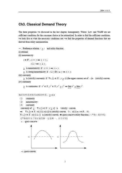
Ch3. Classical Demand TheoryThe three properties we discussed in the last chapter, homogeneity, Walras’ Law, and WARP are not sufficient conditions for the consumer choice to be rationalized. In order to find the sufficient conditions, we look first at what the necessary conditions are; we find the properties of demand functions that are derived from utility maximization.一、Preference relation ( ) and utility function 。
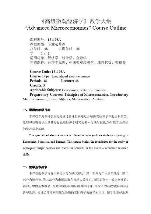
(i) rational: (ii) monotonicity,; .n i i i i x R x y x y x y x y ∈>>⇔>≥⇔≥is monotonicity: if .x y x y >>⇒is strong monotonicity: if &.x y x y x y ≥≠⇒(iii) convexityis (strictly) convexity: if ,{:}x y X y x ∀∈ (the upper contour set of x )is (strictly) convex. (iv) continuityis continuous: if ,;lim lim .nnnnnnn n x X y X x y x y →∞→∞∈∈⇒偏好的性质到效用函数的性质:u → (1) continuity (2) monotonicity:(3) convexity convexity of : ,{:}x y X y x ∀∈ is (strictly )convex.⇒ ,{:()()}x y X u y u x ∀∈≥is (strictly) convex. 令:()u x c R =∈,则:,{:()}c y X u y c ∀∈≥ is (strictly) convex. Î quasi-concave utility function.((严格)拟凹性)(严格拟凹为了保证最佳解一定是唯一,并且可导) u :quasi-concave:u −quasi-convexQuasi-concave and quasi-convex: monotone function; special e.g. line functionAnother proposition: if u is concave (convex) , f is strictly increasing, then f u is quasi-concave (quasi-convex).二、效用最大化问题(utility maximization problem )(UMP)1、 效用最大化问题 给定p ,w ,11max ()s.t. or (budget constraint)xn n u x px w px p x p x ≤=+⋅⋅⋅+性质1:只要u 是连续的,UMP 有解重写UMP {},max ()s.t. :,0xp w u x x B x px w x ∈=≤≥解的存在性和唯一性: B p,w 是闭集,并且有上下界,⇒B p,w 是紧集(compact set ),紧集上的连续函数最大化问题一定有解。
- 1、下载文档前请自行甄别文档内容的完整性,平台不提供额外的编辑、内容补充、找答案等附加服务。
- 2、"仅部分预览"的文档,不可在线预览部分如存在完整性等问题,可反馈申请退款(可完整预览的文档不适用该条件!)。
- 3、如文档侵犯您的权益,请联系客服反馈,我们会尽快为您处理(人工客服工作时间:9:00-18:30)。
Chapter 5 Properties of DemandWhy? Theory – observable characteristics – testing – for future5.1 Relative prices and real incomez Money is a veil. Economists often prefer to measure important economicvariables in real, rather than nominal terms. z Relative pricesj ip p z Relative income jp wz Homogeneity and budget balancedness),1,...,,(),(0),(),(21nn n p w p p p p x w P x t tw tP x w P x =⇒>∀= ),(),(w P w w P Px ∀=5.2 The Slutsky equationz What do we expect from the theory of consumer? --- The law of demandClassical theory: the principle of diminishing marginal utilityz However, Giffen good! It is a product for which, among a poor population, a risein price will lead people to buy even more of the product. Possible examples: the potato in the Irish famine of 1845-1849[Figure 1.19]z Normal good and inferior goodThe “good” is the product for which demand increases in income.0),(>∂∂w w P x i The “bad” is … 0),(<∂∂w w P x iA Giffen good must be inferior, OR/AND an inferior good must be a Giffen good ??z Income effect and substitution effect IE SE TE +=Total effect : (price effect) measures the change of quantity demanded for a goodin response to a change in its price.Substitution effect : measures the effect of relative price change, in which theconsumer substitutes the relatively cheaper good for the relatively expensive good, and remains indifferent after the price change. Income effect :[Figure 1.20]z Theorem 5.1 The Slutsky equation :ww P x w P x p u P x p w P x ij j h i j i ∂∂−∂∂=∂∂∗),(),(),(),( Proof: from last chapter we know: *)),(,(*),(u P e P x u P x i h i =ji j i j h i p u P e w u P e P x p u P e P x p u P x ∂∂∂∂+∂∂=∂∂∗*),(*)),(,(*)),(,(),( w w P v P e u P e ==)),(,(*),(Shephard’s Lemma :)),(,(*),(*),(w P v P x u P x p u P e hj h j j==∂∂ ),()),(,(w P x w P v P x j h j =),(),(),(),(w P x w w P x p w P x p u P x j i j i j h i ∂∂+∂∂=∂∂⇒∗ww P x w P x p u P x p w P x ij j h i j i ∂∂−∂∂=∂∂⇒∗),(),(),(),(z Theorem 5.2 The law of demand :1. Hicksian demand: 0),(≤∂∂ih i p u P x (Negative Own-Substitution Terms)2. Marshallian demand: A decrease in the own price of a normal good will cause quantity demanded to increase. If an own price decrease causes a decrease in quantity demanded, the good must be inferior.Proof: using Shephard’s Lemma and the fact that the expenditure is a concave function. Hence…Classical theory vs. Modern theoryz Theorem 5.3 Symmetric, negative semidefinite (Hicksian) substitutionmatrix()⎟⎟⎟⎟⎟⎟⎠⎞⎜⎜⎜⎜⎜⎜⎝⎛∂∂∂∂∂∂∂∂≡n h n h n n h h p u P x p u P x p u P x p u P x u P ),(...),(:::),(...),(,1111σProof: 1) The order of differentiation of the expenditure function makes nodifference! i j j i p p u P e p p u P e ∂∂∂=∂∂∂),(),(22ihj j h i p u P x p u P x ∂∂=∂∂⇒),(),( 2) ()u P ,σ is simply the Hessian matrix of second-order price partials ofthe expenditure function.z Slutsky matrix⎟⎟⎟⎟⎟⎠⎞⎜⎜⎜⎜⎜⎝⎛∂∂+∂∂∂∂+∂∂∂∂+∂∂∂∂+∂∂),(),(),(...),(),(),(:::),(),(),(...),(),(),(11111111w P x w w P x p w P x w P x w w P x p w P x w P x w w P x p w P x w P x w w P x p w P x n n n n n n n n5.3 Some Elasticity Relationsz A general formula for elasticity: yxx y y x y x e xy ln ln %%∂∂=∂∂=∆∆=z Income Elasticity ),(),(w P x ww w P x i i i ∂∂≡ηz Price Elasticity ),(),(w P x p p w P x i jj i ij ∂∂≡εz Aggregation in consumer demand, where income share10),(=≥≡∑i ii i i i sands ww P x p sEngel aggregation: ∑==ni i i s 11η Cournot aggregation: ∑=−=ni j iji s s 1ε5.4 Integrabilityz We ask a question: if we observe a demand function ),(w P x that has theseproperties (homogeneous of degree zero, satisfy Walras’ law, and have a symmetric and negative semidefinite Slutsky matrix), can we find preferences that rationalize ),(w P x ?-- This integrability problem has a long tradition, beginning with Antonelli 1886.z Why we ask such question?1. On a theoretical level, the properties of demand (homogeneity of degree one,satisfaction of Walras’ law, and a symmetric and negative semidefinite substitution matrix) are not only necessary consequences of the preference-based demand theory, but these are also all of the consequences. As long as consumer demand satisfies these properties, there is some rational preference relation that could have generated this demand.2. The result completes our study of the relation between the preference-basedtheory of demand and the choice-based theory of demand. In general, demand satisfying the weak axiom cannot be rationalized by preferences, because the substitution matrix could be not symmetric. Hence, the result here shows us, that the only thing added to the properties of demand by the rational preference hypothesis, beyond what is implied by the weak axiom, homogeneity of degree one, and Walras’ law, is symmetry of the substitution matrix.3. On a practical level, the result tells us how and when we can recover theinformation of preferences from observation of the consumer’s demand behavior. 4. In empirical studies, it allows us to begin by specifying a tractable demandfunction and then check whether it satisfies the necessary and sufficient conditions. We need not derive the utility function. zTwo steps to recover preferences from demand:1. recovering preferences from the expenditure function ),(u P eTheorem 5.4 Constructing a utility function from an expenditure functionLet ),(w P e be a function satisfying all properties of an expenditure function, then we can construct a utility function by {})(|0max )(u A x u x u ∈≥≡, where{}0),(|)(>>∀≥∈≡+P u P e Px R x u A n2. recovering an expenditure function from ),(w P xTheorem 5.5 Constructing an expenditure function from a demand functionThe necessary and sufficient condition for the recovery of an underlying expenditure function is the symmetric and negative semidefiniteness of the Slutsky equation.At first, we consider the case of two goods. Suppose 12=p without loss of generality, pick an arbitrary point ),,1,(0001u w p .We will now recover the value of the expenditure function 0),1,(101>∀p u p e from following differential equation (to integrate):))(,(),()(1111111p e p x u p x dp p de h == with the initial condition 001)(w p e = For the general case of L commodities, we have a system of partial differential equations:))(,()(...))(,()(11P e P x p P e P e P x p P e L L=∂∂=∂∂ The existence of a solution to above system is guaranteed when 2>L if and only ifits Hessian matrix )(2P e D p is symmetric. ( Frobenius’ theorem)In addition, if a solution exists, as long as ),(w P S is negative semidefinite, it will possess the properties of an expenditure function.The intuition: by changing prices one at a time, we can decompose this problem into L subproblems where only one price changes at each step. Hence, the symmetry of Slutsky matrix implies that the value of expenditure function should not depend on the particular path from the original price to the new price.Example:Suppose there are three goods, the demand function is as follows:3,2,1,),,,(321==i p ww p p p x ii i α, where 1,0321=++>ααααand iWe want to find ()u p p p e ,,,321.We have:()()()321321332211213333122232111321321321)(),()()ln()ln()ln()),(ln(),,()ln()),(ln(),,()ln()),(ln(),,()ln()),(ln(3,2,1,,,,ln 3,2,1,,,,,,,αααααααααααp p p u c u P e u c p p p u P e u p p c p u P e u p p c p u P e u p p c p u P e i p p u p p p e i p u p p p e p u p p p e i i ii i i =⇒+++=⇒⎪⎩⎪⎨⎧+=+=+=⇒==∂∂⇒==∂∂Because the implied demand behavior is independent of strictly increasing transformation, we can choose u u c =)(.Recover a utility function from this expenditure function.{})(|0max )(u A x u x u ∈≥≡, where {}0),(|)(>>∀≥∈≡+P u P e Px R x u A n321321321321),(ααααααp p p Pxu p p up u P e Px ≤⇔=≥ Hence ()321321332211αααp p p x p x p x p x u ++=5.5Welfare analysis。