数字信号处理-第五章
胡广书_数字信号处理题解及电子课件_第5章
π 3. 在实轴但不在圆上,无共轭,角度=0, π 4. 在实轴,但在圆上,无共轭,角度=0,
模<1; 模=1;
在单位圆内 四个零点同时存在, 构成四阶系统.
把该式展开,其系数也是对称的,是具 有线性相位的子系统。
无共轭零点, 有镜象零点
无镜象对称零点, 有共轭零点.
无镜象零点, 也无共轭零点.
− jω n
+
n = ( N +1) / 2
∑
N −1
h ( n )e
− jω n
N −1 + h e 2
N −1 − j ω 2
令:
m = N −1 − n
( N −3) 2 ( N −3) 2 m=0
H (e jω ) 的对称性,有 并利用
H (e jω ) =
则该系统具有线性相位。
上述对称有四种情况:
偶对称
N : even N : odd
第一类 FIR 系统
N : even N : odd
奇对称
第二类 FIR 系统
1. N 为奇数
H (e jω ) = ∑ h(n)e − jω n
n =0 N −1
第一类 FIR 系统
=
( N −3) 2
∑
n=0
h(n)e
幅频
一 阶 全 通 系 统
0 -0.5 -1 -1 0 -1 0 (a) 1
0
0.2 (b)
0.4
1
0.5 -2 0 -3 -4 -0.5
0
0.2 (c)
0.4
0
5
10 (d)
15
20
相频
抽样响应
1 1 0.5 0 -0.5 -1 -1 0 -2 0.5 -4 0 -6 -8 -0.5 0 (a) 1 0 0.5
数字信号处理,第5章课后习题答案
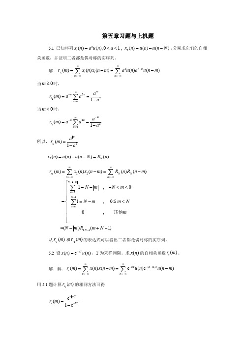
第五章习题与上机题5.1 已知序列12()(),0 1 , ()()()nx n a u n a x n u n u n N =<<=--,分别求它们的自相关函数,并证明二者都是偶对称的实序列。
解:111()()()()()nn mx n n r m x n x n m a u n au n m ∞∞-=-∞=-∞=-=-∑∑当0m ≥时,122()1mmnx n ma r m aaa∞-===-∑ 当0m <时,122()1m mnx n a r m aaa -∞-===-∑ 所以,12()1mx ar m a =-2 ()()()()N x n u n u n N R n =--=22210121()()()()()1,0 =1,00, =()(1)x NN n n N mn N n m N r m x n x n m Rn R n m N m N m N m m Nm N m R m N ∞∞=-∞=-∞--=-=-=-=-⎧=--<<⎪⎪⎪⎪=-≤<⎨⎪⎪⎪⎪⎩-+-∑∑∑∑其他从1()x r m 和2()x r m 的表达式可以看出二者都是偶对称的实序列。
5.2 设()e()nTx n u n -=,T 为采样间隔。
求()x n 的自相关函数()x r m 。
解:解:()()()()e()e ()nTn m T x n n r m x n x n m u n u n m ∞∞---=-∞=-∞=-=-∑∑用5.1题计算1()x r m 的相同方法可得2e()1e m Tx Tr m --=-5.3 已知12()sin(2)sin(2)s s x n A f nT B f nT ππ=+,其中12,,,A B f f 均为常数。
求()x n 的自相关函数()x r m 。
解:解:()x n 可表为)()()(n v n u n x +=的形式,其中)2sin()(11s nT f A n u π=,=)(n v 22sin(2)s A f nT π,)(),(n v n u 的周期分别为 s T f N 111=,sT f N 221=,()x n 的周期N 则是21,N N 的最小公倍数。
第五章 时域离散系统的基本网络结构

本章的主要内容就是描述数字滤波器的基 本网络结构。(IIR、FIR)
引言
时域离散系统或网络可以用差分方程、单 位脉冲响应以及系统函数进行描述。
M
N
y(n) bi x(n i) ai y(n i)
i0
i 1
系统函数H(z)为
M
H (z)
(2) 流图环路中必须存在延时支路;
(3) 节点和支路的数目是有限的。
信号流图表达的系统含义
每个节点连接的有输入支路和输出支路,节点变 量等于所有输入支路的输出之和.
根据信号流图可以求出系统函数(节点法、梅逊 公式法)。
1(n) 2 (n 1) 2 (n) 2 (n 1) 2 (n) x(n) a12 (n) a21n y(n) b21(n) b12 (n) b02(n)
画出H(z)的直接型结构和级联型结构。
级联型
解: 将H(z)进行因式分解,得到: H(z)=(0.6+0.5z-1)(1.6+2z-1+3z-2)
其直接型结构和级联型结构如图所示。
x(n)
0.6
z- 1 0.5
1.6 z- 1
2 z- 1
3
y(n) x(n)
z- 1
z- 1
z- 1
0.96 2
2.8 1.5 y(n)
0 j
y(n)
1 j
z- 1 1j
1 j
z- 11 j
(a)
2 j
z-
1
2
j
(b)
一阶和二阶直接型网络结构 (a)直接型一阶网络结构;(b)直接型二阶网络结构
IIR的级联型例题
数字信号处理-原理实现及应用(高西全-第3版)第5章 信号的相关函数及应用

rxy (m) ryx (m)
性质2 rxy (m) rx (0)ry (0) ExEy
性质3
lim
m
rxy (m)
0
因为一般能量信号都是有限非零时宽的,所以,当 m 时,二者的非零区不重叠, 所以,该性质成立。
信息与通信工程系—数字信号处理
2.自相关函数性质
性质1
若 x(n) 是实信号,则 rx (m)是实偶函数,即
[h(m) h(m)][x(m) x(m)]
rh (m) rx (m)
ry (0) rh (m) rx (m) m0
= rh (n)rx (n m) = rh (n)rx (n)
n
m0 n
系统稳定,则h(n)为能量信号
rh (m) 存在;
如果 rx (m) 存在,则 ry (m) 存在。
观测信号 y(n) x(n) w(n);y(n) 的自相关函 ry (m)
(a) 2
w(n)
0
-2 10 20 30 40 50 60 70 80 90 100 n
(b) 2
y(n)
0
-2
10
20
30
40
50 n
60
70
80
90 100
噪声自相关
(c)
函数导致
1
ry(m)
0
-1
-50 -40 -30 -20 -10
h(m) [x(m) x(m)]
h(m) rx (m)
所以,ryx (m)可以看成线性时不变系统对输入序列的响应输出。
rx (m)
LTI系统 h(n)
ryx (m)
信息与通信工程系—数字信号处理
系统输出信号的自相关函数:
第五章 数字信号处理- 微弱信号处理

第五章微弱信号处理5.1 微弱信号检测技术中气体浓度检测仪中的应用微弱信号不仅意味着信号的幅度小,而且主要指被噪声淹没中的信号。
为了检测被背景噪音淹没的信号,就需要分析噪声产生的原因和规律,研究被测信号的特点、相关性以及噪声的统计特性,以寻找出从背景噪声中检测有用信号的方法。
因此,微弱信号检测技术的首要任务是提高信噪比。
它不同于一般的检测技术,它注重的不是传感器的物理模型和传感原理、相应的信号转换电路和仪表实现方法,而是如何抑制噪声和提高信噪比。
由于被测量的信号微弱,传感器的固有噪声、放大电路及测量仪器的固有噪声以及外界的干扰噪声往往比有用信号的幅度大得多,放大被测信号的过程同时也放大了噪声,而且必然还会附加一些额外的噪声,因此只靠放大是不能把微弱信号检测出来的。
只有在有效地抑制噪声的条件下增大微弱信号的幅度,才能提取出有用的信号。
为了表征噪声对信号的淹没程度,引入信噪比SNR来表示,它指的是信号的有效值S与噪音的有效值N之比。
而评价一种微弱信号检测方法的优劣,经常采用两种指标:一种是信噪改善比SNIR,它等于系统输出端的信噪比SNR和系统输入段oSNR之比。
SNIR越大,表明系统抑制噪声的能力越强。
i另一个指标是检测分辨率,指的是检测仪器指示值可以响应与分辨的最小输入值的变化值。
检测分辨率不同于检测灵敏度,后者表示的是检测系统标定曲线的斜率,定义为输出变化量y∆之比。
一般情况下,∆的输入变化量x∆与引起y灵敏度越高,分辨率越好。
但提高系统的放大倍数虽可提高灵敏度,但却不一定能提高分辨率,因为分辨率要受噪声和误差额制约。
5.1.1 本检测系统的噪声源广义的噪声是扣除被测信号真实值以后的各种测量值,可以分为两类:一是干扰;另一被称为电子噪声(狭义)。
干扰是指被非被测信号或非测量系统所引起的噪声。
从理论上讲,干扰是属于理想上可排除的噪声。
不少干扰源发出的干扰是有规律的,有些具有周期性,有些只是瞬时值。
《信号、系统与数字信号处理》第五章 Z变换与离散系统的频域分析
同理
sinh0nun
1 2
e0n
e0n
un
1 z
2
z
e0
z z e0
z2
z sinh0 2z cosh0
1
z max e0 , e0
2、双边z变换的移位 n0 0
若 xn X z
RX
z
R X
则 x n n0 z n0 X z
RX
z
R X
证明: Z x n n0
n
xT t nT estdt
n
xnT esnT
n
令 z esT 引入新的复变量, 将上式写为
X s s xnT zn
n
此式是复变量 z 的函数(T 是常数),记为
X z xnzn
n
x 2z2 x 1z x0 x1z1 x2z2
Z xn 2un z2 X z z1x1 x 2
3) 若 xn 为因果序列 xnun X z
则 xn mun zm X z
m0
xn
mun
zm
X
z
m1 k 0
xk
z
k
例5-9 求周期序列的单边z变换
解: 周期序列 xn xn rN
m0
令 n 0 ~ N 1 的主值区序列为 x1 n ,
( z 1)
4、指数序列加权
若 xn X z RX z RX
则 an xn X a1z
RX a 1z RX
证:Z an xn an xnzn
n
xn a1z n X z / a
n
RX a 1z RX
a
R X
z
a
R X
利用
数字信号处理 第五章

+ a2 z-1
数字信号处理—第五章
6
举例:二阶数字滤波器
y ( n ) a 1 y ( n 1) a 2 y ( n 2 ) b 0 x ( n )
x(n) b0 +
-1 a1 z
y(n)
+ a2 z-1
数字信号处理—第五章
7
举例:二阶数字滤波器
y ( n ) a 1 y ( n 1) a 2 y ( n 2 ) b 0 x ( n )
z z
2 2
H (z)
1 1k z 1 1k z
1 1
x(n)
H 1(z)
y (n )
H 2(z)
H k (z)
数字信号处理—第五章
22
数字信号处理—第五章
23
IIR数字滤波器的级联型结构优点
1) 每个二阶或一阶子系统单独控制零、极点。 2)级联顺序可交换,零、极点对搭配任意,因此级联 结构不唯一。有限字长对各结构的影响是不一样的, 可通过计算机仿真确定子系统的组合及排序。 3)级联各节之间要有电平的放大和缩小,以使变量值 不会太大或太小。太大可能导致运算溢出;太小可 能导致信噪比太小。 4)级联系统也属于最少延时单元实现,需要最少的存 储器,但乘法次数明显比直接型要多。 4)级联结构中后面的网络输出不会再流到前面,运算 误差积累比直接型小。
数字信号处理—第五章
4
基本单元(数字滤波器结构)有两种表 示方法
数字信号处理—第五章
5
举例:二阶数字滤波器
y ( n ) a 1 y ( n 1) a 2 y ( n 2 ) b 0 x ( n )
x(n) b0 +
数字信号处理第五章-IIR数字滤波器的设计

2、由模平方函数确定系统函数
模拟滤波器幅度响应常用幅度平方函数表示:
| H ( j) |2 H ( j)H *( j)
由于冲击响应h(t)为实函数,H ( j) H *( j)
| H ( j) |2 H ( j)H ( j) H (s)H (s) |s j
H (s)是模拟滤波器的系统函数,是s的有理分式;
分别对应:通带波纹和阻带衰减(阻带波纹)
(4种函数)
只介绍前两种
31
32
33
无论N多大,所 有特性曲线均通 过该点
特性曲线单调减小,N越大,减小越慢 阻
特性曲线单调减小,N越大,减小越快
34
20Nlog2:频率增加一倍,衰减6NdB
35
另外:
36
无论N多大,所 有特性曲线均通 过Ωc点: 衰减3dB, Ωc 为 3dB带宽
8
根据
(线性相位滤波器)
非线性相位滤波器
9
问题:
理想滤波器的幅度特性中,频带之间存 在突变,单位冲击响应是非因果的;
只能用逼近的方法来尽量接近实际的要 求。
滤波器的性能要求以频率响应的幅度特 性的允许误差来表征,如下图:
10
p
11
低通滤波器的频率响应包括:
通带:在通带内,以幅度响应的误差δp逼近 于1;
20
3、数字滤波器设计的基本方法
利用模拟理论进行设计 先按照给定的技术指标设计出模拟滤波 器的系统函数H(s),然后经过一定的变 换得到数字滤波器的系统函数H(z),这实 际上是S平面到Z平面的映射过程: 从时域出发,脉冲响应不变法 从频域出发,双线性变换法 适合于设计幅度特性较规则的滤波器, 如低通、高通等。
由于系统稳定, H(s)的极点一定落在s的左半 平面,所以左半平面的极点一定属于H(s),右 半平面的极点一定属于H(-s)。
- 1、下载文档前请自行甄别文档内容的完整性,平台不提供额外的编辑、内容补充、找答案等附加服务。
- 2、"仅部分预览"的文档,不可在线预览部分如存在完整性等问题,可反馈申请退款(可完整预览的文档不适用该条件!)。
- 3、如文档侵犯您的权益,请联系客服反馈,我们会尽快为您处理(人工客服工作时间:9:00-18:30)。
N / 2 1 n 0
N 1
n even
x(n)W
N / 2 1 n 0 k N
kn N
kn x(n)WN n odd
X (k )
x(2n)W
2 kn N
k ( 2 n 1) x ( 2 n 1 ) W N N / 2 1 n 0 kn x ( 2 n 1 ) W N /2
N / 2 1 n 0
x(2n)W
kn N /2
W
(5.1)
k G ( k ) WN H (k )
where
G(k )
N / 21 n 0
x(2n)W
kn N /2
H (k )
N / 21 n 0
k ( 2 n 1) x ( 2 n 1 ) W N
(5.2)
Both G(k) and H(k) are N/2-point DFT. Although the index k ranges over N values, k = 0 , 1, …, N – 1, each of the sums needs only be computed for k between 0 and N/2 – 1 since G(k) and H(k) are periodic in k with period N/2. After the two DFTs corresponding to the two sums are computed, they are then combined to yield the N-point DFT, X(k). We have seen that the direct computation without exploiting symmetry, N2 complex multiplications (CM)
5.2 Decimation-in-time FFT algorithms
Let N be an integer power of 2, i.e., N = 2m. Since N is an even integer, we can compute X(k) by separating x(n) into two N/2-points sequences consisting of the even numbered points in x(n) and the odd-numbered points in x(n). That is or
N-point computation into the two N/2-point computation. If N/2 is even, as it always is when N is a power of 2, then we can continue to decompose each of the N/2-point DFTs into N/4-point DFTs. That is, G(k) and H(k) can be computed as follows:
G(k )
N / 21 n 0
or
g (n)W
kn N /2
N / 4 1 n 0
g (2n)W
kn N /4
kn N /4
N / 4 1 n 0
k ( 2 n 1) g ( 2 n 1 ) W N /2
G (k )
N / 4 1 n 0
x(4n)W
kn kn X (k ) Rex(n)Re WN Imx(n)Im WN n 0 kn N N 1
j Rex(n)ImW Imx(n)Re W
kn N
The above equation shows that the direct computation of X(k) for each k requires 4N real multiplications (RM) and 4N – 2 real additions (RA). The computation of all the coefficients needs 4N2 RM and N(4N – 2) RA. The computation is large, especially when N is large.
Chapter 5. Computation of the discrete Fou
The discrete Fourier transform (DFT) plays an important role in the analysis, the design, and the implementation of digital signal processing algorithms and systems. One of reasons that Fourier analysis is of such wide-ranging importance in digital signal processing is because of the existence of efficient algorithms for computing the discrete Fourier transform. Recall that the DFT of a finite-duration sequence x(n) is N 1 kn X (k ) x(n)WN , k = 0, 1, …, N – 1, (5-1) n 0 j 2 / N where WN e . The IDFT is
W
k N /2
N / 4 1 n 0
kn x ( 4 n 2 ) W N /4
Similarly,
H (k )
N / 4 1 n 0
x(4n 1)W
kn N /4
W
k N /2
N / 4 1 n 0
kn x ( 4 n 3 ) W N /4
We can continue this procedure until left with only twopoint transforms, this requires m (m = log2N) stages of computation. We have seen that in the original decomposition of an N-point transform into two N/2point transforms, the number of CM and CA required was N+N2/2. When the N/2-point transforms are decomposed into N/4-point transforms, the factor (N/2)2 is replaced by N/2+2(N/4)2, so the overall computation requires N+N+4(N/4)2 CM and CA. If N = 2m, this can be done at most m = log2N times, thus, the number of CM and CA is equal to N log2N.
For this reason, it is important to develop efficient algorithms. Many efforts have been paid on this field. The possibility of greatly reduced computation was overlooked by Cooley and Tukey (1965). This publication touched off a flurry of activity in the application of the DFT to signal processing and resulted in the discovery of a number of computational algorithms known as fast Fourier transform (FFT). The fundamental principle of these algorithms is based on the decomposition of a sequence with length N into successively smaller DFTs. The manner in which this principle is implemented leads to a variety of different algorithms, all with comparable improvements in terms
1 x ( n) N
kn X ( k ) W N k 0 N 1
1 N 1 * kn X ( k ) W N N k 0
*
To indicate the importance of efficient computation schemes, it is instructive to consider the direct computation of the DFT equations. Since x(n) may be complex, we can write
computational efficiency. We will present two basic classes of FFT algorithms. The first one, called decimation-in-time (DIT), derives its name from the fact that in the process of arranging the computation into smaller transformations, the sequences x(n) is decomposed into successively smaller subsequences. The second one is termed as decimation-in-frequency (DIF), which consists of decomposing the DFT coefficients X(k) into smaller subsequences.