Weibull分布
质量管理课程-Weibull分布

案例三
总结词
复杂系统的Weibull分布可靠性评估
详细描述
质量管理课程中,我们还通过案例研究探讨 了复杂系统的Weibull分布可靠性评估。针 对由多个子系统组成的复杂系统,我们首先 识别了各子系统的故障模式和失效机制,然 后使用Weibull分布模型对各子系统的可靠 性进行了评估。最后,我们综合各子系统的 可靠性特征,对整个复杂系统的可靠性进行 了分析和预测。这一案例研究有助于提高我
案例二
总结词
机械部件故障模式的Weibull分布应用
详细描述
在质量管理课程中,我们还探讨了机械部件故障模式的Weibull分布应用。针对不同类 型的机械部件,我们收集了其故障数据,并使用Weibull分布模型进行拟合。通过对比 不同部件的Weibull分布参数,我们分析了各部件的故障模式和可靠性特征,为预防性
Weibull分布的特性
总结词
Weibull分布具有形状参数和尺度参数两个参数,决定了分布 的形状和尺度。
详细描述
Weibull分布有两个参数,一个是形状参数λ(lambda),一个 是尺度参数k。形状参数决定了分布的形状,尺度参数决定了分 布的尺度。当形状参数λ=1时,Weibull分布退化为指数分布。
识别潜在故障模式
通过FMEA分析,识别产品或过程中可能出 现的故障模式。
分析故障影响
评估每种故障模式对产品质量、安全性、可 靠性和其他关键性能指标的影响。
确定风险优先级
根据故障影响程度和发生概率,确定风险优 先级,为改进措施提供依据。
制定预防措施
针对高风险故障模式,制定有效的预防措施, 降低其发生概率或减轻其影响程度。
掌握如何利用软件进行Weibull分布的拟合、分析和绘 图。
r计算weibull分布的尺度和形状参数
r计算weibull分布的尺度和形状参数
在R语言中,可以使用`weibull`函数来计算Weibull分布的尺度和形状参数。
首先,我们需要安装并加载`weibull`包。
如果尚未安装,可以使用以下代码进行安装:
ibull`包:
ibull`函数来拟合Weibull分布。
假设我们有一组数据`x`,我们可以使用以下代码来拟合Weibull分布并计算尺度和形状参数:
r
拟合Weibull分布
fit <- weibull(x, shape = 1, scale = 1)
输出拟合结果
summary(fit)
合结果中,`shape`参数表示形状参数,`scale`参数表示尺度参数。
这些参数可以通过最小化均方误差(MSE)来估计。
在上面的代码中,我们使用默认值1作为初始估计值。
如果需要手动计算尺度和形状参数,可以使用以下公式:
尺度参数(Scale):`scale = 1 / lambda`,其中`lambda`是平均故障时间(MTTF)。
形状参数(Shape):`shape = alpha`,其中`alpha`是形状参数。
在R语言中,可以使用以下代码来计算尺度和形状参数:
x为数据集,可以是寿命数据或其他连续数据
计算形状参数(假设数据符合指数分布)
shape <- 1 指数分布的形状参数为1,对于Weibull分布,形状参数可能需要根据实际情况进行调整
```。
weibull分布风速模型基本构成参数及其作用。

在进行深入探讨Weibull分布风速模型基本构成参数及其作用之前,我们先来简单了解一下Weibull分布。
Weibull分布是由瑞典数学家瓦尔德玛·魏布尔于1951年提出的,用来描述风速、风力等自然现象的统计分布。
1. Weibull分布的基本特征Weibull分布是一种连续概率分布,其密度函数为:\[ f(x;\lambda,k) = \frac{k}{\lambda}\left(\frac{x}{\lambda}\right)^{k-1} e^{-(x/\lambda)^k} \]其中,\( x>0 \),\( \lambda>0 \)为比例参数,\( k>0 \)为形状参数。
Weibull分布的平均值、方差和标准差分别为:\[ \text{E}[X] = \lambda \Gamma(1+\frac{1}{k}) \]\[ \text{Var}[X] = \lambda^2 \left[ \Gamma(1+\frac{2}{k}) -(\Gamma(1+\frac{1}{k}))^2 \right] \]\[ \text{Std}[X] = \lambda \sqrt{\left[ \Gamma(1+\frac{2}{k}) - (\Gamma(1+\frac{1}{k}))^2 \right]} \]其中,\( \Gamma \)为Gamma函数。
2. Weibull分布的构成参数Weibull分布的构成参数包括比例参数\( \lambda \)和形状参数\( k \)。
比例参数\( \lambda \)反映了分布的尺度,它决定了分布的位置,即控制了平均值的大小。
形状参数\( k \)决定了分布的形状,描述了分布的偏斜性。
当\( k>1 \)时,分布呈现右偏态,当\( k<1 \)时,分布呈现左偏态,当\( k=1 \)时,分布呈现对称性。
3. Weibull分布的作用Weibull分布在风能、风电等领域得到了广泛的应用。
韦伯预测(Weibull Forecast)

Confidential
5
参考书籍
书名: 书名:新韦伯分析手册 作 者:瓦拉第.韦伯 出 版 社:鼎茂出版社 出版日期:2007-03-15 版 本:4版 I S B N :9789574143658
. 相关网站:/blog/weibull4tw新韦伯分 析手册第四版副标题:可靠度与寿命预测,安全,存活, 风险,成本和保固理赔的统计分析.
韦伯分布 (Weibull distribution)
韦伯分布(Weibull distribution), 韦伯分布 又称韦氏分布 威布尔分布 韦氏分布或威布尔分布 韦氏分布 威布尔分布,是可靠 性分析和寿命检验的理论基础.
韦伯分布历史 韦伯分布
1. 1927年,Fréchet (1927)首先给出这一分布 的定义. 2. 1933年,Rosin和Rammler在研究碎末的分 布时,第一次应用了韦伯分布(Rosin, P.; Rammler, E. (1933), "The Laws Governing the Fineness of Powdered Coal", Journal of the Institute of Fuel 7: 29 - 36.). 3. 1951年,瑞典工程师,数学家Waloddi Waloddi Weibull(1887-1979)详细解释了这一分布, Weibull 于是,该分布便以他的名字命名为Weibull Distribution.
Confidential
6
�
Confidential
3
韦伯分布应用 韦伯分布
生存分析 工业制造 极值理论 预测天气 可靠性和失效分析 雷达系统 拟合度 量化寿险模型的重复索赔 预测技术变革 风速
威布尔Weibull分布的寿命试验方法

轮船正招式成商立局,标志着中国新式航运业的诞生。
(2)1900年前后,民间兴办的各种轮船航运公司近百家,几乎都是
在列强排挤中艰难求生。
2.航空
(1)起步:1918年,附设在福建马尾造船厂的海军飞机工程处开始
研制 。
(2)发展水:上1飞918机年,北洋政府在交通部下设“
”;此后十年间,航空事业获得较快发展。
1.李鸿章1872年在上海创办轮船招商局,“前10年盈和,成
为长江上重要商局,招商局和英商太古、怡和三家呈鼎立
之势”。这说明该企业的创办
()
A.打破了外商对中国航运业的垄断
B.阻止了外国对中国的经济侵略
C.标志着中国近代化的起步
D.使李鸿章转变为民族资本家
解析:李鸿章是地主阶级的代表,并未转化为民族资本家; 洋务运动标志着中国近代化的开端,但不是具体以某个企业 的创办为标志;洋务运动中民用企业的创办在一定程度上抵 制了列强的经济侵略,但是并未能阻止其侵略。故B、C、D 三项表述都有错误。 答案:A
選擇可靠性,并輸入 “0.90”, 時間項輸入 “500”
分布選擇 “Weibull”
輸入 “8.55”
允許的最大失效數 項輸入 “0”
每個單元的檢驗次 數項輸入 “600”
結果分析
所需測試的樣本數量是6 個,這6個樣本在600小時 測試時間內不能失效,該 試驗計划的實際置信水 平是95.05%.
3.发展 (1)原因: ①甲午战争以后列强激烈争夺在华铁路的 修。筑权 ②修路成为中国人 救的亡强图烈存愿望。 (2)成果:1909年 京建张成铁通路车;民国以后,各条商路修筑 权收归国有。 4.制约因素 政潮迭起,军阀混战,社会经济凋敝,铁路建设始终未入 正轨。
韦伯分布介绍

韋伯分佈韋伯分佈(Weibull distribution)以指數分佈為一特例。
其p.d.f.為其中α,β>0。
以表此分佈, 有二參數α,β, α為尺度參數, β為形狀參數。
若取β=1, 則得分佈, 以表之。
底下給出一些韋伯分佈p.d.f.之圖形。
韋伯分佈是瑞典物理學家Waloddi Weibull, 為發展強化材料的理論, 於西元1939年所引進, 是一較新的分佈。
在可靠度理論及有關壽命檢定問題裡, 常少不了韋伯分佈的影子。
分佈的分佈函數為期望值與變異數分別為Characteristic Effects of the Shape Parameter, β, for the Weibull DistributionThe Weibull shape parameter, β, is also known as the slope. This is because the value of β is equal to the slope of the regressed line in a probability plot. Different values of the shape parameter can have marked effects on the behavior of the distribution. In fact, some values of the shape parameter will cause the distribution equations to reduce to those of other distributions. For example, when β = 1, the pdf of the three-parameter Weibull reduces to that of thetwo-parameter exponential distribution or:where failure rate.The parameter β is a pure number, i.e. it is dimensionless.The Effect of β on the pdfFigure 6-1 shows the effect of different values of the shape parameter, β, on the shape of the pdf. One can see that the shape of the pdf can take on a variety of forms based on the value of β.Figure 6-1: The effect of the Weibull shape parameter on the pdf.For 0 < β1:∙As (or γ),∙As , .∙f(T) decreases monotonically and is convex as T increases beyond the value of γ.∙The mode is non-existent.For β > 1:∙f(T) = 0 at T = 0 (or γ).∙f(T) increases as (the mode) and decreases thereafter.∙For β < 2.6 the Weibull pdf is positively skewed (has a right tail), for 2.6 < β < 3.7 its coefficient of skewness approaches zero (no tail). Consequently, it may approximate the normal pdf, and for β > 3.7 it is negatively skewed (left tail).The way the value of β relates to the physical behavior of the items being modeled becomes more apparent when weobserve how its different values affect the reliability and failure rate functions. Note that for β = 0.999, f(0) = , but for β = 1.001, f(0) = 0. This abrupt shift is what complicates MLE estimation when β is close to one.The Effect ofβ on the cdf and Reliability FunctionFigure 6-2: Effect of β on the cdf on a Weibull probability plot with a fixed value of η.Figure 6-2 shows the effect of the value of β on the cdf, as manifested in the Weibull probability plot. It is easy to see why this parameter is sometimes referred to as the slope. Note that the models represented by the three lines all have the same value of η. Figure 6-3 shows the effects of these varied values of β on the reliability plot, which is a linear analog of the probability plot.Figure 6-3: The effect of values of β on the Weibull reliability plot.∙R(T) decreases sharply and monotonically for 0 < β < 1 and is convex.∙For β = 1, R(T) decreases monotonically but less sharply than for 0 < β < 1 and is convex.∙For β > 1, R(T) decreases as T increases. As wear-out sets in, the curve goes through an inflection point and decreases sharply.The Effect of β on the Weibull Failure Rate FunctionThe value of β has a marked effect on the failure rate of the Weibull distribution and inferences can be drawn about a population's failure characteristics just by considering whether the value of β is less than, equal to, or greater than one.Figure 6-4: The effect of β on the Weibull failure rate function.As indicated by Figure 6-4, populations with β < 1 exhibit a failure rate that decreases with time, populations with β = 1 have a constant failure rate (consistent with the exponential distribution) and populations with β > 1 have a failure rate that increases with time. All three life stages of the bathtub curve can be modeled with the Weibull distribution and varying values of β.The Weibull failure rate for 0 < β < 1 is unbounded at T = 0 (or γ). The failure rate, λ(T), decreases thereaftermonotonically and is convex, approaching the value of zero as or λ( ) = 0. This behavior makes it suitable for representing the failure rate of units exhibiting early-type failures, for which the failure ratedecreases with age. When encountering such behavior in a manufactured product, it may be indicative of problems in the production process, inadequate burn-in, substandard parts and components, or problems with packaging and shipping.For β = 1, λ(T) yields a constant value of or:This makes it suitable for representing the failure rate of chance-type failures and the useful life period failure rate of units.For β > 1, λ(T) increases as T increases and becomes suitable for representing the failure rate of units exhibiting wear-out type failures. For 1 < β < 2, the λ(T) curve is concave, consequently the failure rate increases at a decreasing rate as T increases.For β = 2 there emerges a straight line relationship between λ(T) and T, starting at a value of λ(T) = 0 at T = γ, andincreasing thereafter with a slope of . Consequently, the failure rate increases at a constant rate as T increases. Furthermore, if η = 1 the slope becomes equal to 2, and when γ = 0, λ(T) becomes a straight line which passes through the origin with a slope of 2. Note that at β = 2, the Weibull distribution equations reduce to that of the Rayleigh distribution.When β > 2, the λ(T) curve is convex, with its slope increasing as T increases. Consequently, the failure rate increases at an increasing rate as T increases indicating wear-out life.TopCharacteristic Effects of the Scale Parameter, η, for the Weibull DistributionFigure 6-5: The effects of η on the Weibull pdf for a common β.A change in the scale parameter η has the same effect on the distribution as a change of the abscissa scale. Increasing the value of η while holding β constant has the effect of stretching out the pdf. Since the area under a pdf curve is a constant value of one, the "peak" of the pdf curve will also decrease with the increase of η, as indicated in Figure 6-5.∙If η is increased while β and γ are kept the same, the distribution gets stretched out to the right and its height decreases, while maintaining its shape and location.∙If η is decreased while β and γ are kept the same, the distribution gets pushed in towards the left (i.e. towards its beginning or towards 0 or γ), and its height increases.∙η has the same units as T, such as hours, miles, cycles, actuations, etc.TopCharacteristic Effects of the Location Parameter, γ, for the Weibull DistributionThe location parameter, γ, as the name implies, locates the distribution along the abscissa. Changing the value of γ has the effect of "sliding" the distribution and its associated function either to the right (if γ > 0) or to the left (if γ < 0).Figure 6-6: The effect of a positive location parameter, γ, on the position of the Weibull pdf.∙When γ = 0, the distribution starts at T = 0 or at the origin.∙If γ > 0, the distribution starts at the location γ to the right of the origin.∙If γ < 0, the distribution starts at the location γ to the left of the origin.∙γ provides an estimate of the earliest time-to-failure of such units.∙The life period 0 to +γ is a failure free operating period of such units.∙The parameter γ may assume all values and provides an estimate of the earliest time a failure may be observed. A negative γ may indicate that failures have occurred prior to the beginning of the test, namelyduring production, in storage, in transit, during checkout prior to the start of a mission, or prior to actual use.∙γ has the same units as T, such as hours, miles, cycles, actuations, etc.。
16种常见概率分布概率密度函数意义及其应用
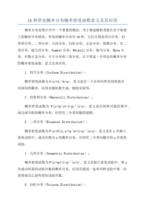
16种常见概率分布概率密度函数意义及其应用概率分布是统计学中一个重要的概念,用于描述随机变量在各个取值上的概率分布情况。
常见的概率分布有16种,它们分别是均匀分布、伯努利分布、二项分布、几何分布、泊松分布、正态分布、指数分布、负二项分布、超几何分布、Gumbel分布、Weibull分布、伽马分布、Beta分布、对数正态分布、卡方分布和三角分布。
以下将逐一介绍这些概率分布的概率密度函数、意义及其应用。
1. 均匀分布(Uniform Distribution):概率密度函数为f(x)=1/(b-a),意义是在一个区间内所有的取值具有相同的概率,应用有随机数生成、模拟实验等。
2. 伯努利分布(Bernoulli Distribution):概率密度函数为P(x)=p^x*(1-p)^(1-x),意义是在两种可能结果中,成功或失败的概率分布,应用有二分类问题的建模。
3. 二项分布(Binomial Distribution):概率密度函数为P(x)=C(n,x)*p^x*(1-p)^(n-x),意义是在n次独立重复试验中,成功次数为x的概率分布,应用有二分类问题中的n次重复试验。
4. 几何分布(Geometric Distribution):概率密度函数为P(x)=p*(1-p)^(x-1),意义是独立重复试验中,第x次成功所需的试验次数的概率分布,应用有描述一连串同样试验中第一次获得成功之前所需的试验次数。
5. 泊松分布(Poisson Distribution):概率密度函数为P(x)=(e^(-λ)*λ^x)/x!,意义是在给定时间或空间内事件发生的次数的概率分布,应用有描述单位时间或单位空间内的事件计数问题。
6. 正态分布(Normal Distribution):概率密度函数为P(x) = (1 / sqrt(2πσ^2)) * e^(-(x-μ)^2 / (2σ^2)),意义是描述连续变量的概率分布,应用广泛,例如测量误差、人口身高等。
正态分布指数分布对数正态分布和威布尔分布函数及其在工程分析中的应用
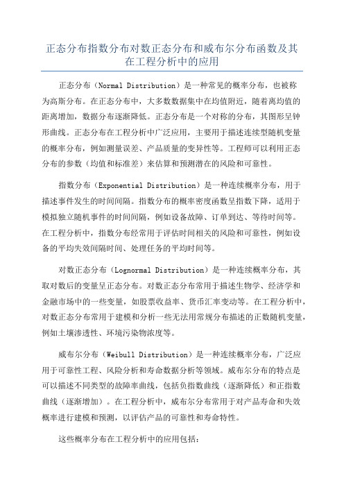
正态分布指数分布对数正态分布和威布尔分布函数及其在工程分析中的应用正态分布(Normal Distribution)是一种常见的概率分布,也被称为高斯分布。
在正态分布中,大多数数据集中在均值附近,随着离均值的距离增加,数据分布逐渐降低。
正态分布是一个对称的分布,其图形呈钟形曲线。
正态分布在工程分析中广泛应用,主要用于描述连续型随机变量的概率分布,例如测量误差、产品质量的变异性等。
工程师可以利用正态分布的参数(均值和标准差)来估算和预测潜在的风险和可靠性。
指数分布(Exponential Distribution)是一种连续概率分布,用于描述事件发生的时间间隔。
指数分布的概率密度函数呈指数下降,适用于模拟独立随机事件的时间间隔,例如设备故障、订单到达、等待时间等。
在工程分析中,指数分布经常用于评估时间相关的风险和可靠性,例如设备的平均失效间隔时间、处理任务的平均时间等。
对数正态分布(Lognormal Distribution)是一种连续概率分布,其取对数后的变量呈正态分布。
对数正态分布常用于描述生物学、经济学和金融市场中的一些变量,如股票收益率、货币汇率变动等。
在工程分析中,对数正态分布常用于建模和分析一些无法用常规分布描述的正数随机变量,例如土壤渗透性、环境污染物浓度等。
威布尔分布(Weibull Distribution)是一种连续概率分布,广泛应用于可靠性工程、风险分析和寿命数据分析等领域。
威布尔分布的特点是可以描述不同类型的故障率曲线,包括负指数曲线(逐渐降低)和正指数曲线(逐渐增加)。
在工程分析中,威布尔分布常用于对产品寿命和失效概率进行建模和预测,以评估产品的可靠性和寿命特性。
这些概率分布在工程分析中的应用包括:1.风险评估:通过对输入变量的分布进行建模,可以使用这些概率分布来评估不同风险情景的概率和可能性。
例如,在工程项目中,可以使用正态分布来估算成本、时间和质量方面的风险。
2.可靠性分析:通过使用威布尔分布和指数分布来模拟和分析设备失效时间和寿命数据,工程师可以评估设备的可靠性和耐用性,进而制定相应的维护策略和计划。
- 1、下载文档前请自行甄别文档内容的完整性,平台不提供额外的编辑、内容补充、找答案等附加服务。
- 2、"仅部分预览"的文档,不可在线预览部分如存在完整性等问题,可反馈申请退款(可完整预览的文档不适用该条件!)。
- 3、如文档侵犯您的权益,请联系客服反馈,我们会尽快为您处理(人工客服工作时间:9:00-18:30)。
Weibull分布(韦伯分布)
(2006-07-04 22:04:01)
转载
分类:学习
Weibull分布,又称韦伯分布、韦氏分布或威布尔分布,由瑞典物理学家Wallodi Weibull于1939年引进,是可靠性分析及寿命检验的理论基础。
Weibull分布能被应用于很多形式,包括1参数、2参数、3参数或混合Weibull。
3参数的该分布由形状、尺度(范围)和位置三个参数决定。
其中形状参数是最重要的参数,决定分布密度曲线的基本形状,尺度参数起放大或缩小曲线的作用,但不影响分布的形状。
另外,通过改变形状参数可以表示不同阶段的失效情况;也可以作为许多其他分布的近似,如,可将形状参数设为合适的值近似正态、对数正态、指数等分布。
形状参数通常在[1,7]间取值。
一般由W(α,β)表示2个参数的Weibull分布,其分布函数为:
,其中x>0,α、β>0。
可以看出有两个参数α、β,其中β为形状参数,α为尺度参数。
若取β为1,则F(x)为指数分布。
Weibull分布的概率密度函数(pdf)为:。
Weibull双参数的PDF分布见上图。
(自己做的,有点粗糙)
下面我们以其pdf图看Weibull分布各参数的作用。
下图是形状参数β对pdf的影响(α固定):
下图为尺度参数α对pdf的影响(β固定),横轴为变量x,纵轴为f(x):
另外,由于Weibull分布可以近似表示其他别的分布,eg,β=1时,F(x)为指数分布。
将其用到复杂网络中,则此时对应指数网络?当β逐渐增大时,是不是对应分布极不均匀的无尺度网络?这样的话可以通过调整一个参数构造不同的网络?
而**人的层次故障节点动态模型就是因此而引入Weibull分布(1参数)的吧?这样的话,β大的网络发生层次故障的规模比较大就可以理解了。
再继续深入分析。