计量--工具变量
计量经济学-工具变量
利用E(zii)=0,在大样本下可得到:
~1
zi yi zi xi
关于0 的估计,仍用~0 Y ~1X 完成。
这种求模型参数估计量的方法称为工具变 量法(instrumental variable method),相应的估 计 量 称 为 工 具 变 量 法 估 计 量 ( instrumental variable (IV) estimator)。
CONSP 0 1GDPP 由于:居民人均消费支出(CONSP)与人 均国内生产总值(GDPP)相互影响,因此,
容易判断GDPP与同期相关(往往是 正相关),OLS估计量有偏并且是非一致的
(低估截距项而高估计斜率项 )。
OLS估计结果:
(13.51) (53.47) R2=0.9927 F=2859.23 DW=0.5503 SSR=23240.7
用OLS估计模型,相当于用xi去乘模型两边、对i求 和、再略去xii项后得到正规方程:
xi yi 1 xi2
解得:
ˆ1
xi yi xi2
(*)
由于Cov(Xi,i)=E(Xii)=0,意味着大样本下: (xii)/n0
表明大样本下:
ˆ1
xi yi xi2
2. 工具变量并没有替代模型中的解释变量, 只是在估计过程中作为“工具”被使用。
上述工具变量法估计过程可等价地分解成下 面的两步OLS回归:
第一步,用OLS法进行X关于工具变量Z的回归:
Xˆ i ˆ0 ˆ1Zi
Yˆi ~0 ~1 Xˆ i
容易验证仍有:
~1
zi yi zi xi
如果用GDPPt-1为工具变量,可得如下工具 变量法估计结果:
北大计量经济学讲义-工具变量与两阶段最小二乘法
nehS naY ,scirtemonocE etaidemretnI
计估SLO的1b到得们我�时x=z当 . 1b
计估�时在存VI当 noitamitsE :elbaliavA si VI na nehW
91
nehS naY ,scirtemonocE etaidemretnI
计估�时在存VI当 noitamitsE :elbaliavA si VI na nehW
�量变具工用使何为 ?selbairaV latnemurtsnI esU yhW
7
nehS naY ,scirtemonocE etaidemretnI
题问差误量测的典经决解来用可VI�且而 melborp selbairav-ni-srorre cissalc eht evlos ot desu eb nac VI ,yllanoitiddA � 差偏量变漏遗决解来用以可VI�以所 saib elbairav dettimo fo melborp eht sserdda ot desu eb nac VI ,suhT �
�
定决资工�子例 noitanimreted egaw :elpmaxE
41
nehS naY ,scirtemonocE etaidemretnI
。关相项差误和育教与时同它。不 .mret rorre eht dna noitacude htob htiw setalerroc tI .oN � �吗量变具工的好是QI ?tnemurtsni doog a QI sI �
。计估致一的1b是计估VI明证律定数 大用应以可�时立成 )5.51(和 )4.51(定假当 .srebmun egral fo wal eht gniylppa retfa ,1b rof tnetsisnoc si rotamitse VI eht taht wohs nac eno ,dloh )5.51( dna )4.51( snoitpmussa nehW �
北大计量经济学讲义-工具变量与两阶段最小二乘法
large numbers. 当假定(15.4) 和(15.5) 成立时,可以应用大
数定律证明IV估计是b1的一致估计。
Intermediate Econometrics,
That is, Cov(z,u) = 0 (15.4) 即Cov(z,u) = 0
Intermediate Econometrics,
Yan Shen
8
Instrumental Variable: Who qualifies? 什么样的变量可以作为IV?
The instrument must be correlated with the endogenous variable x 工具变量应与内生变量 x 相关
Intermediate Econometrics,
Yan Shen
5
Why Use Instrumental Variables? 为何使用工具变量?
Instrumental Variables (IV) estimation is used when your model has endogenous x’s 当模型解释变量具有内生性时,使用工具 变量估计
Suppose the true model regresses log(wage) on education (educ) and ability (abil). 假定真实模型将对数工资对教育和能力回归
Now ability is unobserved, and the proxy, IQ, is not available. 现在能力不可观测,而且没有代理变量IQ
b1 . 当z=x时,我们得到b1的OLS估计
计量经济学工具变量IV (2SLS)
A New Approach to the Omitted Variable Problem
We have talked about the problem of omitted variable bias (in Ch.3), and have shown that it will lead to inconsistency, for
Compute the predicted values of xi, x^i, where
x^i = ^0 + ^1 zi, i = 1,…,n.
(2) Replace xi by x^i in the regression of interest:
regress y on x^i using OLS:
The instrumental variable detects movements in xi that
are uncorrelated with ui, and use these to estimate 1.
Two conditions for a valid instrument
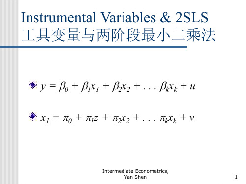
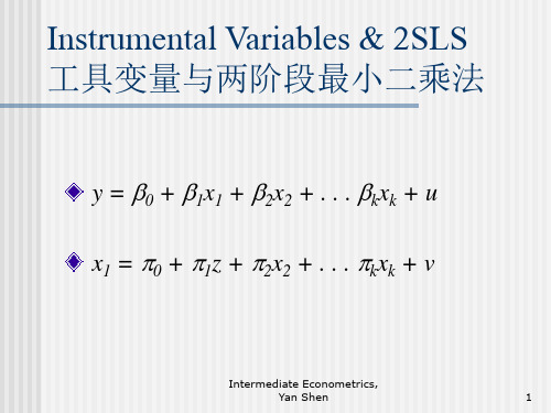
yi = 0 + 1xi + ui
Suppose for now that you have such a zi (we’ll discuss how to find instrumental variables later)
How can you use zi to estimate 1?
We will explain this in two ways
Parent’s education, or number of siblings might be an instrument for educ
第15章-工具变量

第 9 章则证明了,对无法观测解释变量给出适 宜的代理变量,能消除 (或至少减轻)遗漏变量 偏误。不幸的是,我们不是总能得到适宜的代 理变量。
在前面两章,我们解释了在出现不随时间而 变化的遗漏变量情况下, 如何对面板数据应 用固定效应估计或一阶差分来估计随时间而 变化的自变量的影响。尽管这些方法非常有 用,可我们不是总能获得面板数据。
举例来说,考虑成年劳动者的工资方程中存 在无法观测之能力因素的问题。一个简单的 模型为: log(wage)=β 0+β 1educ+β 2abil+e 其中,e 是误差项。
在第 9 章中,我们证明了在某些假定下,如 何用诸如 IQ 的代理变量代替能力,从而通过 以下回归可得到一致估计量 log(wage)对 educ,IQ 回归 然而假定不能得到适当的代理变量(或它不 具备足以获取 1 一致估计量所需的性质)。
如我们在第 2 篇中所示,OLS 可以应用于时 间序列数据,而工具变量法也一样可以。15.7 节讨论了在时间序列数据中应用 IV 法时出现 的一些特殊问题。在 15.8 节中,我们将论述 其在混合横截面和面板数据上的应用。
15.1 动机:简单回归模型中的遗漏变量
面对可能发生的遗漏变量偏误(或无法观测 异质性),迄令为止我们已讨论了三种选择: (1)我们可以忽略此问题,承受有偏而又不 一致估计量的结果;
现在我们来论证,工具变量的可用性能够用于 一致地估计方程 (15. 2)中的参数。具体而言, 我们将说明式(15.4) 与式(15.5) 中的假定足以识 别参数 1 。在这一点上,参数的识别 (identification)意味着我们可以根据总体矩写 出 1 ,而总体矩可用样本数据进行估计。
为了根据总体协方差写出 1 ,我们利用方程 (15.2):z 与 y 之间的协方差为
计量经济学工具变量IVSLS
计量经济学工具变量IVSLS计量经济学中的工具变量(Instrumental Variable, IV)和两阶段最小二乘法(TwoStage Least Squares, 2SLS)是解决内生性问题的重要方法。
本文将从基本概念、理论依据、估计方法、应用案例以及优缺点等方面,对IVSLS进行详细阐述。
一、基本概念1. 内生性问题内生性问题是指模型中的解释变量与误差项存在相关性的问题。
这种相关性可能导致普通最小二乘法(Ordinary Least Squares, OLS)估计的偏误,进而影响模型的准确性和可靠性。
内生性问题主要源于以下几个方面:(1)遗漏变量:模型中未包含对因变量有影响的变量。
(2)同时性:解释变量与因变量同时变化,导致估计偏误。
(3)测量误差:解释变量或因变量的测量误差可能导致内生性问题。
2. 工具变量工具变量(Instrumental Variable, IV)是一种用于解决内生性问题的方法。
工具变量需满足以下条件:(1)与内生解释变量高度相关。
(2)与误差项无关。
(3)与模型中其他解释变量无关。
3. 两阶段最小二乘法(2SLS)两阶段最小二乘法(TwoStage Least Squares, 2SLS)是一种利用工具变量解决内生性问题的估计方法。
该方法分为两个阶段:第一阶段:利用工具变量对内生解释变量进行回归,得到其预测值。
第二阶段:将第一阶段的预测值代入原模型,使用最小二乘法进行估计。
二、理论依据1. 工具变量的有效性工具变量的有效性取决于其与内生解释变量的相关性以及与误差项的无关性。
如果工具变量与内生解释变量的相关性较弱,那么其估计结果将不准确;如果工具变量与误差项相关,那么其估计结果将存在偏误。
2. 2SLS估计的渐近性质在满足一定条件下,2SLS估计具有以下渐近性质:(1)一致性:当样本容量趋于无穷大时,2SLS估计的值将收敛于真实参数值。
(2)渐进正态性:当样本容量趋于无穷大时,2SLS估计的分布将趋于正态分布。
计量经济学总结:计量工具变量伍德里奇
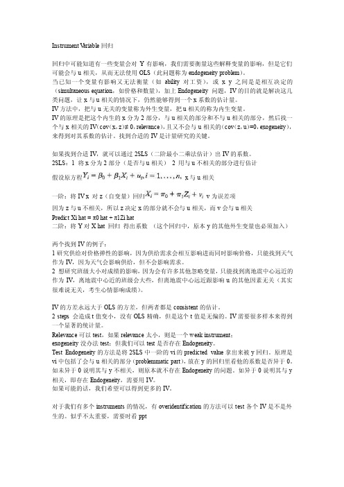
Instrument V ariable回归回归中可能知道有一些变量会对Y有影响,我们需要衡量这些解释变量的影响,但是它们可能会与u相关,从而无法使用OLS(此问题称为endogeneity problem)。
当已知一个变量有影响又无法衡量(如ability对工资),或x y之间是是相互决定的(simultaneous equation,如价格和数量),加上Endogeneity 问题,IV的目的就是解决这几类问题,让x与u相关的情况下,仍然能够得到一个x系数的估计量。
IV方法中,把与u无关的变量称为外生变量,把u相关的称为内生变量。
IV的原理是把这个内生的x分为2部分,与u相关的部分和不与u相关的部分,然后找一个与x相关的IV(cov(x,z)≠ 0,relevance),且又不会与u相关的(cov(z,u)=0,exogeneity),来得到对其系数的估计。
找到合适的IV是计量研究的关键。
如果找到合适IV,就可以通过2SLS(二阶最小二乘法估计)出IV的系数。
2SLS:1 将x分为2部分(是否与u相关)2 用与u不相关的部分进行估计假设原方程x与u相关一阶:将IV x 对z(自变量)回归v为误差项因为z与u不相关,所以z决定x的部分就不会与u相关,而v会与u相关Predict Xi hat = π0 hat + π1Zi hat二阶:将Y对X hat 回归得出系数(这个回归中,原本y的其他外生变量也必须加入)两个找到IV的例子:1研究供给对价格弹性的影响,因为供给需求会相互影响进而同时影响价格,只能找到天气作为IV,因为天气会影响供给,但不会影响需求。
2 想研究班级大小对成绩的影响,因为会有许多其他忽略变量,只能找到离地震中心远近的作为IV,离地震中心近的班级会大些,但离地震中心远近跟影响u的其他因素无关(其实很难说无关,考生心情影响成绩)。
IV的方差永远大于OLS的方差,但两者都是consistent的估计。
工具变量是什么意思
工具变量是什么意思
工具变量的意思是:一个计量经济学的概念,它的出现是为了克服普通最小二乘法中的内生性问题。
在这里,内生性是指回归模型中的解释变量(X)和随机扰动项(δ)相关。
工具变量(英语:instrumental variable,简称“IV”)也称为“仪器变量”或“辅助变量”,是经济学、计量经济学、流行病学和相关学科中无法实现可控实验的时候,用于估计模型因果关系的方法。
工具变量(英语:instrumental variable,简称“IV”)也称为“仪器变量”或“辅助变量”,是经济学、计量经济学、流行病学和相关学科中无法实现可控实验的时,用于估计模型因果关系的方法。
在回归模型中,当解释变量与误差项存在相关性(内生性问题),使用工具变量法能够得到一致的估计量。
内生性问题一般产生于被忽略变量问题或者测量误差问题。
当内生性问题出现时,常见的线性回归模型会出现不一致的估计量。
此时,如果存在工具变量,那么人们仍然可以得到一致的估计量。
根据定义,工具变量应该是一个不属于原解释方程并且与内生解释变量相关的变量。
在线性模型中,一个有效的工具变量应该满足以下两点:
此变量和内生解释变量存在相关性;
此变量和误差项不相关,也就是说工具变量严格外生。
- 1、下载文档前请自行甄别文档内容的完整性,平台不提供额外的编辑、内容补充、找答案等附加服务。
- 2、"仅部分预览"的文档,不可在线预览部分如存在完整性等问题,可反馈申请退款(可完整预览的文档不适用该条件!)。
- 3、如文档侵犯您的权益,请联系客服反馈,我们会尽快为您处理(人工客服工作时间:9:00-18:30)。
which introduces a variable z that is associated with x but not u. It is still the case that z and y will be correlated, but the only source of such correlation is the indirect path of z being correlated with x which in turn determines y . The more direct path of z being a regressor in the model for y is ruled out. More formally, a variable z is called an instrument or instrumental variable for the regressor x in the scalar regression model y = x + u if (1) z is uncorrelated with the error u;and (2) z is correlated with the regressor x. The rst assumption excludes the instrument z from being a regressor in the model for y , since if instead y depended on both x and z and y is regressed on x alone then z is being absorbed into the error so that z will then be correlated with the error. The second assumption requires that there is some association between the instrument and the variable being instrumented. Examples of an Instrument In many microeconometric applications it is dif cult to nd legitimate instruments. Here we provide two examples. Suppose we want to estimate the response of market demand to exogenous changes in market price. Quantity demanded clearly depends on price, but prices are not exogenously given since they are determined in part by market demand. A suitable instrument for price is a variable that is correlated with price but does not directly effect quantity demanded. An obvious candidate is a variable that effects market supply, since this also effect prices, but is not a direct determinant of demand. An example is a measure of favorable growing conditions if an agricultural product is being modelled. The choice of instrument here is uncontroversial, provided favorable growing conditions do not directly effect demand, and is helped greatly by the formal economic model of supply and demand. Next suppose we want to estimate the returns to exogenous changes in schooling. Most observational data sets lack measures of individual ability, so regression of earnings on schooling has error that includes unobserved ability and hence is
where there is no association between x and u.
36
CHAPTER 4. LINEAR MODELS
But in some situations there may be an association between regressors and errors. For example, consider regression of earnings (y ) on years of schooling (x). The error term u embodies all factors other than schooling that determine earnings, such as ability. Suppose a person has a high level of u, due to high (unobserved) ability. This increases earnings, since y = x + u. But it may also lead to higher levels of x, since schooling is likely to be higher for those with high ability. A more appropriate path diagram is then the following x " u ! y %
4.8. INSTRUMENTAL VARIABLES De nition of an Instrument
37
A crude experimental or treatment approach is still possible using observational data, provided there exists an instrument z that has the property that changes in z are associated with changes in x but do not led to change in y (aside from the indirect route via x). This leads to the following path diagram z ! x " u ! y %
4.8.2
Instrumental Variable
The inconsistency of OLS is due to endogeneity of x, meaning that changes in x are associated not only with changes in y but also changes in the error u. What is needed is a method to generate only exogenous variation in x. An obvious way is through an experiment, but for most economics applications experiments are too expensive or even infeasible.
where u is an error term. Regression of y on x yields OLS estimate b of . Standard regression results make the assumption that the regressors are uncorrelated with the errors in the model (4.43). Then the only effect of x on y is a direct effect via the term x. We have the following path analysis diagram x u ! y %
4.8.1
InHale Waihona Puke onsistency of OLS
Consider the scalar regression model with dependent variable y and single regressor x. The goal of regression analysis is to estimate the conditional mean function E[y jx]. A linear conditional mean model, without intercept for notational convenience, speci es E[y jx] = x: (4.42) This model without intercept nests the model with intercept if dependent and regressor variables are measured as deviations from their respective means. Interest lies in obtaining a consistent estimate of as this gives the change in the conditional mean given an exogenous change in x. For example, interest may lie in the effect in earnings due to an increase in schooling due to exogenous reasons, such as an increase in the minimum school leaving age, that are not a choice of the individual. The OLS regression model speci es y = x + u; (4.43)