The Large N Limit of the (2,0) Superconformal Field Theory

合集下载

张胜利-TheHGI-南京理工大学

张胜利邮箱：zhangslvip@通讯地址：南京市玄武区孝陵卫200号材料科学与工程学院，邮编：210094主要研究方向：1.二维半导体精细结构的XAFS实验和模拟相结合的研究；2.新型光电信息功能材料的设计和电子结构性质研究；3.低维纳米材料结构与物理化学性质的第一性原理研究。

主持科研项目：1. 国家自然科学青年基金项目，过渡金属二硫属化物范德华异质结的组装、能带调控和光学性质研究，2015.1-2017.12，主持(在研)。

2. 江苏省科技计划项目-青年项目，类石墨烯TMDCs范德华异质结能带调控和光学性质研究，2014.7-2017.6，主持(在研)。

3. 中国博士后科研资助计划项目(2014M551594)，过渡金属二硫属化物范德华异质结的理论设计与物性调控，2014.9-2016.9，主持(在研)。

4. 江苏省博士后科研资助计划项目(1402154C)，新型二维VIB族硫属化合物层状复合材料的设计和性能调控，2014.11-2016.11，主持(在研)。

研究工作经历：2013/7－至今，南京理工大学，材料科学与工程学院，讲师；2008/09 – 2013/06 北京化工大学，计算材料方向, 博士。

教学工作：《新材料技术概论》，《纳米CMOS集成电路设计与加工》和《半导体器件TCAD设计》代表性学术论文:2014Antimonene: Semimetal-semiconductor and Indirect-direct Band Gap Transitions, Angewandte Chemie International Edition, 2014, Accepted. (IF=11.336)phase transition between metallic and semiconducting single-layer MoS2 and WS2 through size effects, Physical Chemistry Chemical Physics 2014, On-line, DOI: 10.1039/c4cp04775c. (IF=4.198)storage for B/n-codoped graphyne, RSC Advances, 4, 54879, 2014. (IF=3.708)24. Yousheng Zou, Haipeng Wang, Shengli Zhang, Dong Lou, Yuhui Dong, Xiufeng Song, Haibo Zeng. Structural, electrical and optical properties of Mg-doped CuAlO 2 films by pulsed laser deposition. RSC Advances, 4, 41294, 2014. (IF=3.708)23. Xiaoming Li, Shengli Zhang, Sergei A Kulinich, Yanli Liu, Haibo Zeng. Engineering surface states ofcarbon dots to achieve controllable luminescence for solid-luminescent composites and sensitiveBe2+ detection. Scientific Reports, 4, 4976-4983, 2014. (IF=5.078)22. Lihong Zhang, Shengli Zhang, Peng Wang, Chuan Liu, Shiping Huang, Huiping Tian. The effect of electric field on Ti-decorated graphyne for hydrogen storage. Computational and Theoretical Chemistry, 1035, 68-75, 2014. (IF=1.368)21. Xiaoli Du, Chuan Liu, Shengli Zhang, Peng Wang, Shiping Huang, Huiping Tian. Structural, magnetic and electronic properties of FenPt13-n clusters with n=0-13: A first-principle study. Journal of Magnetism and Magnetic Materials, 369, 27-33, 2014. (IF=2.002)201320. Shengli Zhang, Yonghong Zhang, Shiping Huang, Peng Wang, Huiping Tian. First-principles study of cubane-type ZnO: Another ZnO polymorph. Chemical Physics Letters, 556, 102-105, 2013.(IF=1.991)19. Shengli Zha ng, Yonghong Zhang, Shiping Huang, Peng Wang and Huiping Tian. Mechanistic investigations on the adsorption of thiophene over cubane–type Zn3NiO4 bimetallic oxide. Applied Surface Science, 258, 10148-10153, 2013. (IF=2.538)18. Chuan Liu, Shengli Zhang, Shiping Huang, Peng Wang, Huiping Tian. Structure, electronic characteristic and thermodynamic properties of K2ZnH4 hydride crystal: A first–principles study.Journal of Alloys and Compounds, 549, 30-37, 2013. (IF=2.726)17. Jia Li, Shengli Zhang, Shiping Huang, Peng Wang, Huiping Tian. Structural, electronic and thermodynamic properties of R3ZnH5(R=K, Rb, Cs): A first–Principle calculation. Journal of Solid State Chemistry, 198, 433-439, 2013. (IF=2.200)16. Zheng Wu, Yonghong Zhang, Shiping Huang, Shengli Zhang. The structural and electronic properties of assembled CdTe Multi–cage nanochains. Computational Materials Science, 68, 238-244, 2013. (IF=1.879)15. Peng Wang, Mingxia Yang, Shengli Zhang, Shiping Huang, Huiping Tian. Density functional theory study of the electronic and magnetic properties of Mn–doped (MgO)n (n=2–10) clusters. Chinese Journal Chemical Physics, 1, 35-42, 2013. (IF=0.720)14. Jiali Jiang, Shengli Zhang, Shiping Huang, Peng Wang, Huiping Tian. Density functional theory studies of Yb-, Ca- and Sr-substituted Mg2NiH4 hydrides. Computational Materials Science, 7, 55-64, 2013. (IF=1.879)13. Ping Cheng, Shengli Zhang, Peng Wang, Shiping Huang, Huiping Tian. First-principles investigation of thiophene adsorption on Ni13 and Zn@Ni12 putational and Theoretical Chemistry, 1020, 136-142, 2013. (IF=1.368)12. Chuan Liu, Shengli Zha ng, Peng Wang, Shiping Huang, Huiping Tian. Confinement effects on structural, electronic properties and dehydrogenation thermodynamics of LiBH4. International Journal of Hydrogen Energy, 20, 8367-8375, 2013. (IF=2.930)11. Yonghong Zhang, Hui Ding, Chuan Liu, Shengli Zhang, Shiping Huang. Significant effects of graphite fragments on hydrogen storage performances of LiBH4: A first-principlesapproach. International Journal of Hydrogen Energy, 38, 13717-13727, 2013. (IF=2.930)201210. Shengli Zhang, Yonghong Zhang, Shiping Huang, Chunru Wang, Theoretical investigationsof sp–sp2 hybridized zero–dimensional fullerenynes. Nanoscale，4, 2839-2842, 2012. (IF=6.739)9. Hui Ding, Sh engli Zhang, Yonghong Zhang, Shiping Huang, Effects of nonmetal element (B, C and Si) additives in Mg2Ni hydrogen storage alloy.International Journal of Hydrogen Energy, 37, 6700-6713, 2012. (IF=2.930)8. Yonghong Zhang, Xiaozhen Zheng, Shengli Zhang, Shiping Huang, Peng Wang, Huiping Tian. Bare and Ni decorated Al12N12cage as materials for hydrogen storage: Density functionalcalculation. International Journal of Hydrogen Energy, 37, 12411-12419, 2012. (IF=2.930)20117. Shengli Zhang, Yonghong Zhang, Shiping Huang, Liang Qiao, Shansheng Yu, Weitao Zheng, Field emission mechanism of island−shape Graphene–BN nanocomposite. Journal of Physical Chemistry C, 115, 9471-9476, 2011. (IF=4.835)6. Shengli Zhang, Yonghong Zhang, Shiping Huang, Hui Liu, Peng Wang, Huiping Tian.Theoretical investigation of growth, stability, and electronic properties of beaded ZnO nanoclusters. Journal of Materials Chemistry, 21, 16905-16910, 2011. (IF=6.626)5. Shengli Zhang, Yonghong Zhang, Shiping Huang, Hui Liu, Peng Wang, Huiping Tian. Theoretical investigation of electronic structure and field emission properties of ZnO–CNT nanocontacts. Carbon, 49, 3835-3841, 2011. (IF=6.160)4. Rui Jin, Shengli Zhang,Yonghong Zhang, Shiping Huang, Peng Wang, Huiping Tian. Theoretical investigation of adsorption and dissociation of H2 on (ZrO2)n (n=1–6) clusters. International Journal of Hydrogen Energy, 36, 9069-9078, 2011. (IF=2.930)20103. Shengli Zhang, Yonghong Zhang, Shiping Huang, Hui Liu, Peng Wang, Huiping Tian, First–principles study of field emission properties of Graphene–ZnO nanocomposite. Journal of Physical Chemistry C, 114, 19284-19288, 2010. (IF=4.835)2. Shengli Zhang, Yonghong Zhang, Shiping Huang, Hui Liu, Huiping Tian, First-principles study of structural, electronic and vibrational properties of aluminum-doped silica nanotubes. Chemical Physics Letters, 498, 172-177, 2010. (IF=1.991)1. Shengli Zhang, Yonghong Zhang, Shiping Huang, Peng Wang and Huiping Tian. Molecular dynamics simulations of silica nanotube: structural and vibrational properties under differenttemperatures. Chinese Journal of Chemical Physics, 23, 497-503, 2010. (IF=0.720)。

Two-Dimensional Gas of Massless Dirac Fermions in Graphene

Two-Dimensional Gas of Massless Dirac Fermions in Graphene K.S. Novoselov1, A.K. Geim1, S.V. Morozov2, D. Jiang1, M.I. Katsnelson3, I.V. Grigorieva1, S.V. Dubonos2, A.A. Firsov21Manchester Centre for Mesoscience and Nanotechnology, University of Manchester, Manchester, M13 9PL, UK2Institute for Microelectronics Technology, 142432, Chernogolovka, Russia3Institute for Molecules and Materials, Radboud University of Nijmegen, Toernooiveld 1, 6525 ED Nijmegen, the NetherlandsElectronic properties of materials are commonly described by quasiparticles that behave as nonrelativistic electrons with a finite mass and obey the Schrödinger equation. Here we report a condensed matter system where electron transport is essentially governed by the Dirac equation and charge carriers mimic relativistic particles with zero mass and an effective “speed of light” c∗ ≈106m/s. Our studies of graphene – a single atomic layer of carbon – have revealed a variety of unusual phenomena characteristic of two-dimensional (2D) Dirac fermions. In particular, we have observed that a) the integer quantum Hall effect in graphene is anomalous in that it occurs at halfinteger filling factors; b) graphene’s conductivity never falls below a minimum value corresponding to the conductance quantum e2/h, even when carrier concentrations tend to zero; c) the cyclotron mass mc of massless carriers with energy E in graphene is described by equation E =mcc∗2; and d) Shubnikov-de Haas oscillations in graphene exhibit a phase shift of π due to Berry’s phase.Graphene is a monolayer of carbon atoms packed into a dense honeycomb crystal structure that can be viewed as either an individual atomic plane extracted from graphite or unrolled single-wall carbon nanotubes or as a giant flat fullerene molecule. This material was not studied experimentally before and, until recently [1,2], presumed not to exist. To obtain graphene samples, we used the original procedures described in [1], which involve micromechanical cleavage of graphite followed by identification and selection of monolayers using a combination of optical, scanning-electron and atomic-force microscopies. The selected graphene films were further processed into multi-terminal devices such as the one shown in Fig. 1, following standard microfabrication procedures [2]. Despite being only one atom thick and unprotected from the environment, our graphene devices remain stable under ambient conditions and exhibit high mobility of charge carriers. Below we focus on the physics of “ideal” (single-layer) graphene which has a different electronic structure and exhibits properties qualitatively different from those characteristic of either ultra-thin graphite films (which are semimetals and whose material properties were studied recently [2-5]) or even of our other devices consisting of just two layers of graphene (see further). Figure 1 shows the electric field effect [2-4] in graphene. Its conductivity σ increases linearly with increasing gate voltage Vg for both polarities and the Hall effect changes its sign at Vg ≈0. This behaviour shows that substantial concentrations of electrons (holes) are induced by positive (negative) gate voltages. Away from the transition region Vg ≈0, Hall coefficient RH = 1/ne varies as 1/Vg where n is the concentration of electrons or holes and e the electron charge. The linear dependence 1/RH ∝Vg yields n =α·Vg with α ≈7.3·1010cm-2/V, in agreement with the theoretical estimate n/Vg ≈7.2·1010cm-2/V for the surface charge density induced by the field effect (see Fig. 1’s caption). The agreement indicates that all the induced carriers are mobile and there are no trapped charges in graphene. From the linear dependence σ(Vg) we found carrier mobilities µ =σ/ne, whichreached up to 5,000 cm2/Vs for both electrons and holes, were independent of temperature T between 10 and 100K and probably still limited by defects in parent graphite. To characterise graphene further, we studied Shubnikov-de Haas oscillations (SdHO). Figure 2 shows examples of these oscillations for different magnetic fields B, gate voltages and temperatures. Unlike ultra-thin graphite [2], graphene exhibits only one set of SdHO for both electrons and holes. By using standard fan diagrams [2,3], we have determined the fundamental SdHO frequency BF for various Vg. The resulting dependence of BF as a function of n is plotted in Fig. 3a. Both carriers exhibit the same linear dependence BF = β·n with β ≈1.04·10-15 T·m2 (±2%). Theoretically, for any 2D system β is defined only by its degeneracy f so that BF =φ0n/f, where φ0 =4.14·10-15 T·m2 is the flux quantum. Comparison with the experiment yields f =4, in agreement with the double-spin and double-valley degeneracy expected for graphene [6,7] (cf. caption of Fig. 2). Note however an anomalous feature of SdHO in graphene, which is their phase. In contrast to conventional metals, graphene’s longitudinal resistance ρxx(B) exhibits maxima rather than minima at integer values of the Landau filling factor ν (Fig. 2a). Fig. 3b emphasizes this fact by comparing the phase of SdHO in graphene with that in a thin graphite film [2]. The origin of the “odd” phase is explained below. Another unusual feature of 2D transport in graphene clearly reveals itself in the T-dependence of SdHO (Fig. 2b). Indeed, with increasing T the oscillations at high Vg (high n) decay more rapidly. One can see that the last oscillation (Vg ≈100V) becomes practically invisible already at 80K whereas the first one (Vg <10V) clearly survives at 140K and, in fact, remains notable even at room temperature. To quantify this behaviour we measured the T-dependence of SdHO’s amplitude at various gate voltages and magnetic fields. The results could be fitted accurately (Fig. 3c) by the standard expression T/sinh(2π2kBTmc/heB), which yielded mc varying between ≈ 0.02 and 0.07m0 (m0 is the free electron mass). Changes in mc are well described by a square-root dependence mc ∝n1/2 (Fig. 3d). To explain the observed behaviour of mc, we refer to the semiclassical expressions BF = (h/2πe)S(E) and mc =(h2/2π)∂S(E)/∂E where S(E) =πk2 is the area in k-space of the orbits at the Fermi energy E(k) [8]. Combining these expressions with the experimentally-found dependences mc ∝n1/2 and BF =(h/4e)n it is straightforward to show that S must be proportional to E2 which yields E ∝k. Hence, the data in Fig. 3 unambiguously prove the linear dispersion E =hkc∗ for both electrons and holes with a common origin at E =0 [6,7]. Furthermore, the above equations also imply mc =E/c∗2 =(h2n/4πc∗2)1/2 and the best fit to our data yields c∗ ≈1⋅106 m/s, in agreement with band structure calculations [6,7]. The employed semiclassical model is fully justified by a recent theory for graphene [9], which shows that SdHO’s amplitude can indeed be described by the above expression T/sinh(2π2kBTmc/heB) with mc =E/c∗2. Note that, even though the linear spectrum of fermions in graphene (Fig. 3e) implies zero rest mass, their cyclotron mass is not zero. The unusual response of massless fermions to magnetic field is highlighted further by their behaviour in the high-field limit where SdHO evolve into the quantum Hall effect (QHE). Figure 4 shows Hall conductivity σxy of graphene plotted as a function of electron and hole concentrations in a constant field B. Pronounced QHE plateaux are clearly seen but, surprisingly, they do not occur in the expected sequence σxy =(4e2/h)N where N is integer. On the contrary, the plateaux correspond to half-integer ν so that the first plateau occurs at 2e2/h and the sequence is (4e2/h)(N + ½). Note that the transition from the lowest hole (ν =–½) to lowest electron (ν =+½) Landau level (LL) in graphene requires the same number of carriers (∆n =4B/φ0 ≈1.2·1012cm-2) as the transition between other nearest levels (cf. distances between minima in ρxx). This results in a ladder of equidistant steps in σxy which are not interrupted when passing through zero. To emphasize this highly unusual behaviour, Fig. 4 also shows σxy for a graphite film consisting of only two graphene layers where the sequence of plateaux returns to normal and the first plateau is at 4e2/h, as in the conventional QHE. We attribute this qualitative transition between graphene and its two-layer counterpart to the fact that fermions in the latter exhibit a finite mass near n ≈0 (as found experimentally; to be published elsewhere) and can no longer be described as massless Dirac particles. 2The half-integer QHE in graphene has recently been suggested by two theory groups [10,11], stimulated by our work on thin graphite films [2] but unaware of the present experiment. The effect is single-particle and intimately related to subtle properties of massless Dirac fermions, in particular, to the existence of both electron- and hole-like Landau states at exactly zero energy [912]. The latter can be viewed as a direct consequence of the Atiyah-Singer index theorem that plays an important role in quantum field theory and the theory of superstrings [13,14]. For the case of 2D massless Dirac fermions, the theorem guarantees the existence of Landau states at E=0 by relating the difference in the number of such states with opposite chiralities to the total flux through the system (note that magnetic field can also be inhomogeneous). To explain the half-integer QHE qualitatively, we invoke the formal expression [9-12] for the energy of massless relativistic fermions in quantized fields, EN =[2ehc∗2B(N +½ ±½)]1/2. In QED, sign ± describes two spins whereas in the case of graphene it refers to “pseudospins”. The latter have nothing to do with the real spin but are “built in” the Dirac-like spectrum of graphene, and their origin can be traced to the presence of two carbon sublattices. The above formula shows that the lowest LL (N =0) appears at E =0 (in agreement with the index theorem) and accommodates fermions with only one (minus) projection of the pseudospin. All other levels N ≥1 are occupied by fermions with both (±) pseudospins. This implies that for N =0 the degeneracy is half of that for any other N. Alternatively, one can say that all LL have the same “compound” degeneracy but zeroenergy LL is shared equally by electrons and holes. As a result the first Hall plateau occurs at half the normal filling and, oddly, both ν = –½ and +½ correspond to the same LL (N =0). All other levels have normal degeneracy 4B/φ0 and, therefore, remain shifted by the same ½ from the standard sequence. This explains the QHE at ν =N + ½ and, at the same time, the “odd” phase of SdHO (minima in ρxx correspond to plateaux in ρxy and, hence, occur at half-integer ν; see Figs. 2&3), in agreement with theory [9-12]. Note however that from another perspective the phase shift can be viewed as the direct manifestation of Berry’s phase acquired by Dirac fermions moving in magnetic field [15,16]. Finally, we return to zero-field behaviour and discuss another feature related to graphene’s relativistic-like spectrum. The spectrum implies vanishing concentrations of both carriers near the Dirac point E =0 (Fig. 3e), which suggests that low-T resistivity of the zero-gap semiconductor should diverge at Vg ≈0. However, neither of our devices showed such behaviour. On the contrary, in the transition region between holes and electrons graphene’s conductivity never falls below a well-defined value, practically independent of T between 4 and 100K. Fig. 1c plots values of the maximum resistivity ρmax(B =0) found in 15 different devices, which within an experimental error of ≈15% all exhibit ρmax ≈6.5kΩ, independent of their mobility that varies by a factor of 10. Given the quadruple degeneracy f, it is obvious to associate ρmax with h/fe2 =6.45kΩ where h/e2 is the resistance quantum. We emphasize that it is the resistivity (or conductivity) rather than resistance (or conductance), which is quantized in graphene (i.e., resistance R measured experimentally was not quantized but scaled in the usual manner as R =ρL/w with changing length L and width w of our devices). Thus, the effect is completely different from the conductance quantization observed previously in quantum transport experiments. However surprising, the minimum conductivity is an intrinsic property of electronic systems described by the Dirac equation [17-20]. It is due to the fact that, in the presence of disorder, localization effects in such systems are strongly suppressed and emerge only at exponentially large length scales. Assuming the absence of localization, the observed minimum conductivity can be explained qualitatively by invoking Mott’s argument [21] that mean-free-path l of charge carriers in a metal can never be shorter that their wavelength λF. Then, σ =neµ can be re-written as σ = (e2/h)kFl and, hence, σ cannot be smaller than ≈e2/h per each type of carriers. This argument is known to have failed for 2D systems with a parabolic spectrum where disorder leads to localization and eventually to insulating behaviour [17,18]. For the case of 2D Dirac fermions, no localization is expected [17-20] and, accordingly, Mott’s argument can be used. Although there is a broad theoretical consensus [18-23,10,11] that a 2D gas of Dirac fermions should exhibit a minimum 3conductivity of about e2/h, this quantization was not expected to be accurate and most theories suggest a value of ≈e2/πh, in disagreement with the experiment. In conclusion, graphene exhibits electronic properties distinctive for a 2D gas of particles described by the Dirac rather than Schrödinger equation. This 2D system is not only interesting in itself but also allows one to access – in a condensed matter experiment – the subtle and rich physics of quantum electrodynamics [24-27] and provides a bench-top setting for studies of phenomena relevant to cosmology and astrophysics [27,28].1. Novoselov, K.S. et al. PNAS 102, 10451 (2005). 2. Novoselov, K.S. et al. Science 306, 666 (2004); cond-mat/0505319. 3. Zhang, Y., Small, J.P., Amori, M.E.S. & Kim, P. Phys. Rev. Lett. 94, 176803 (2005). 4. Berger, C. et al. J. Phys. Chem. B, 108, 19912 (2004). 5. Bunch, J.S., Yaish, Y., Brink, M., Bolotin, K. & McEuen, P.L. Nanoletters 5, 287 (2005). 6. Dresselhaus, M.S. & Dresselhaus, G. Adv. Phys. 51, 1 (2002). 7. Brandt, N.B., Chudinov, S.M. & Ponomarev, Y.G. Semimetals 1: Graphite and Its Compounds (North-Holland, Amsterdam, 1988). 8. Vonsovsky, S.V. and Katsnelson, M.I. Quantum Solid State Physics (Springer, New York, 1989). 9. Gusynin, V.P. & Sharapov, S.G. Phys. Rev. B 71, 125124 (2005). 10. Gusynin, V.P. & Sharapov, S.G. cond-mat/0506575. 11. Peres, N.M.R., Guinea, F. & Castro Neto, A.H. cond-mat/0506709. 12. Zheng, Y. & Ando, T. Phys. Rev. B 65, 245420 (2002). 13. Kaku, M. Introduction to Superstrings (Springer, New York, 1988). 14. Nakahara, M. Geometry, Topology and Physics (IOP Publishing, Bristol, 1990). 15. Mikitik, G. P. & Sharlai, Yu.V. Phys. Rev. Lett. 82, 2147 (1999). 16. Luk’yanchuk, I.A. & Kopelevich, Y. Phys. Rev. Lett. 93, 166402 (2004). 17. Abrahams, E., Anderson, P.W., Licciardello, D.C. & Ramakrishnan, T.V. Phys. Rev. Lett. 42, 673 (1979). 18. Fradkin, E. Phys. Rev. B 33, 3263 (1986). 19. Lee, P.A. Phys. Rev. Lett. 71, 1887 (1993). 20. Ziegler, K. Phys. Rev. Lett. 80, 3113 (1998). 21. Mott, N.F. & Davis, E.A. Electron Processes in Non-Crystalline Materials (Clarendon Press, Oxford, 1979). 22. Morita, Y. & Hatsugai, Y. Phys. Rev. Lett. 79, 3728 (1997). 23. Nersesyan, A.A., Tsvelik, A.M. & Wenger, F. Phys. Rev. Lett. 72, 2628 (1997). 24. Rose, M.E. Relativistic Electron Theory (John Wiley, New York, 1961). 25. Berestetskii, V.B., Lifshitz, E.M. & Pitaevskii, L.P. Relativistic Quantum Theory (Pergamon Press, Oxford, 1971). 26. Lai, D. Rev. Mod. Phys. 73, 629 (2001). 27. Fradkin, E. Field Theories of Condensed Matter Systems (Westview Press, Oxford, 1997). 28. Volovik, G.E. The Universe in a Helium Droplet (Clarendon Press, Oxford, 2003).Acknowledgements This research was supported by the EPSRC (UK). We are most grateful to L. Glazman, V. Falko, S. Sharapov and A. Castro Netto for helpful discussions. K.S.N. was supported by Leverhulme Trust. S.V.M., S.V.D. and A.A.F. acknowledge support from the Russian Academy of Science and INTAS.43µ (m2/Vs)0.8c4P0.4 22 σ (1/kΩ)10K0 0 1/RH(T/kΩ) 1 2ρmax (h/4e2)1-5010 Vg (V) 50 -10ab 0 -100-500 Vg (V)50100Figure 1. Electric field effect in graphene. a, Scanning electron microscope image of one of our experimental devices (width of the central wire is 0.2µm). False colours are chosen to match real colours as seen in an optical microscope for larger areas of the same materials. Changes in graphene’s conductivity σ (main panel) and Hall coefficient RH (b) as a function of gate voltage Vg. σ and RH were measured in magnetic fields B =0 and 2T, respectively. The induced carrier concentrations n are described by [2] n/Vg =ε0ε/te where ε0 and ε are permittivities of free space and SiO2, respectively, and t ≈300 nm is the thickness of SiO2 on top of the Si wafer used as a substrate. RH = 1/ne is inverted to emphasize the linear dependence n ∝Vg. 1/RH diverges at small n because the Hall effect changes its sign around Vg =0 indicating a transition between electrons and holes. Note that the transition region (RH ≈ 0) was often shifted from zero Vg due to chemical doping [2] but annealing of our devices in vacuum normally allowed us to eliminate the shift. The extrapolation of the linear slopes σ(Vg) for electrons and holes results in their intersection at a value of σ indistinguishable from zero. c, Maximum values of resistivity ρ =1/σ (circles) exhibited by devices with different mobilites µ (left y-axis). The histogram (orange background) shows the number P of devices exhibiting ρmax within 10% intervals around the average value of ≈h/4e2. Several of the devices shown were made from 2 or 3 layers of graphene indicating that the quantized minimum conductivity is a robust effect and does not require “ideal” graphene.ρxx (kΩ)0.60 aVg = -60V4B (T)810K12∆σxx (1/kΩ)0.4 1ν=4 140K 80K B =12T0 b 0 25 50 Vg (V) 7520K100Figure 2. Quantum oscillations in graphene. SdHO at constant gate voltage Vg as a function of magnetic field B (a) and at constant B as a function of Vg (b). Because µ does not change much with Vg, the constant-B measurements (at a constant ωcτ =µB) were found more informative. Panel b illustrates that SdHO in graphene are more sensitive to T at high carrier concentrations. The ∆σxx-curves were obtained by subtracting a smooth (nearly linear) increase in σ with increasing Vg and are shifted for clarity. SdHO periodicity ∆Vg in a constant B is determined by the density of states at each Landau level (α∆Vg = fB/φ0) which for the observed periodicity of ≈15.8V at B =12T yields a quadruple degeneracy. Arrows in a indicate integer ν (e.g., ν =4 corresponds to 10.9T) as found from SdHO frequency BF ≈43.5T. Note the absence of any significant contribution of universal conductance fluctuations (see also Fig. 1) and weak localization magnetoresistance, which are normally intrinsic for 2D materials with so high resistivity.75 BF (T) 500.2 0.11/B (1/T)b5 10 N 1/2025 a 0 0.061dmc /m00.04∆0.02 0c0 0 T (K) 150n =0e-6-3036Figure 3. Dirac fermions of graphene. a, Dependence of BF on carrier concentration n (positive n correspond to electrons; negative to holes). b, Examples of fan diagrams used in our analysis [2] to find BF. N is the number associated with different minima of oscillations. Lower and upper curves are for graphene (sample of Fig. 2a) and a 5-nm-thick film of graphite with a similar value of BF, respectively. Note that the curves extrapolate to different origins; namely, to N = ½ and 0. In graphene, curves for all n extrapolate to N = ½ (cf. [2]). This indicates a phase shift of π with respect to the conventional Landau quantization in metals. The shift is due to Berry’s phase [9,15]. c, Examples of the behaviour of SdHO amplitude ∆ (symbols) as a function of T for mc ≈0.069 and 0.023m0; solid curves are best fits. d, Cyclotron mass mc of electrons and holes as a function of their concentration. Symbols are experimental data, solid curves the best fit to theory. e, Electronic spectrum of graphene, as inferred experimentally and in agreement with theory. This is the spectrum of a zero-gap 2D semiconductor that describes massless Dirac fermions with c∗ 300 times less than the speed of light.n (1012 cm-2)σxy (4e2/h)4 3 2 -2 1 -1 -2 -3 2 44Kn7/ 5/ 3/ 1/2 2 2 210 ρxx (kΩ)-4σxy (4e2/h)0-1/2 -3/2 -5/2514T0-7/2 -4 -2 0 2 4 n (1012 cm-2)Figure 4. Quantum Hall effect for massless Dirac fermions. Hall conductivity σxy and longitudinal resistivity ρxx of graphene as a function of their concentration at B =14T. σxy =(4e2/h)ν is calculated from the measured dependences of ρxy(Vg) and ρxx(Vg) as σxy = ρxy/(ρxy + ρxx)2. The behaviour of 1/ρxy is similar but exhibits a discontinuity at Vg ≈0, which is avoided by plotting σxy. Inset: σxy in “two-layer graphene” where the quantization sequence is normal and occurs at integer ν. The latter shows that the half-integer QHE is exclusive to “ideal” graphene.。

The Renormalized Trajectory of the O(N) Non-linear Sigma Model

H(
0
0
;
0
Y P ( ; 0) =
x0
;c0 ;::) =
Z
D P(
0
x0
; 0 )e H( ; ;c;::);
k
P Px2x
(4)Βιβλιοθήκη 0xx2x0 x
k ; (5)
2. THE FIXED POINT ACTION
The path integral of the O(N) non-linear sigma R Q model on the lattice is given by H), where x is a twoZ = x D x exp( dimensional lattice vector to label the Rsites, x is N R +an Q component scalar eld, and D x = 1 d (1 2 ) is the O(N) invariant meax 1 x x sure. The lattice hamiltonian H is not unique. The only constraints come from the symmetries of the system and the fact that it ought to reduce in the classical continuum limit to the continuum hamiltonian. The lattice hamiltonian with these constraints can be parametrized as
The Renormalized Trajectory of the O(N) Non-linear Sigma Model

随机树大偏差

Adv.Appl.Prob.41,845–873(2009)Printed in Northern Ireland©Applied Probability Trust2009 LARGE DEVIATIONS FOR THE LEAVESIN SOME RANDOM TREESWLODEK BRYC∗∗∗andDA VID MINDA,∗∗∗∗University of CincinnatiSUNDER SETHURAMAN,∗∗∗∗Iowa State UniversityAbstractLarge deviation principles and related results are given for a class of Markov chainsassociated to the‘leaves’in random recursive trees and preferential attachment randomgraphs,as well as the‘cherries’inYule trees.In particular,the method of proof,combininganalytic and Dupuis–Ellis-type path arguments,allows for an explicit computation of thelarge deviation pressure.Keywords:Large deviation;central limit;preferential attachment;planar oriented;uniformly random trees;leaves;cherries;Yule;random Stirling permutations2000Mathematics Subject Classiﬁcation:Primary60F10Secondary05C801.Introduction and resultsIn this paper we consider large deviations and related laws of large numbers and central limit theorems for a class of Markov chains associated to the number of leaves,or nodes of degree one,in preferential attachment random graphs and random recursive trees,and also the number of‘cherries’,or pairs of leaves with a common parent,in Yule trees.These random graphs model various networks such as pyramid schemes,chemical polymerization,the Internet, social structures,genealogical families,among others.In particular,the leaf and cherry counts in these models are of interest,and have concrete interpretations.Deﬁne the nondecreasing Markov chain{Z n:n≥1}starting from the initial state Z1= k0≥0by its one-step transitionsPr(Z n+1−Z n=v|Z n)=⎧⎪⎨⎪⎩1−Z ns nif v=1,Z ns nif v=0,(1.1)where{s n:n≥1}is a sequence of positive numbers such thats n≥k0+n−1and s nn→αfor some1<α<∞(1.2)Received1October2008;revision received14April2009.∗Postal address:Department of Mathematical Sciences,University of Cincinnati,2855Campus Way,PO Box210025, Cincinnati,OH45221-0025,USA.∗∗Email address:wlodzimierz.bryc@∗∗∗Email address:david.minda@∗∗∗∗Postal address:Department of Mathematics,396Carver Hall,Iowa State University,Ames,IA50011,USA. Email address:sethuram@845846W.BRYC ET AL. with convention that0/0=0.Additionally,we also consider two special sequences:s n=n,α=1,and k0=0,1,(1.3)ands n=n2,α=12,and k0=0.(1.4)The Markov chain Z n,with respect to certain s n s andαs,will be seen to represent the count of leaves in preferential attachment and recursive trees,and the count of cherries in Yule trees. For most of these models,a law of large numbers(LLN)and a central limit theorem(CLT) with respect to Z n have been proved.Then,characterizing the associated large deviations is a natural problem which gives insight into the properties of rare events,and seems less studied in random graphs.Previous large deviations work on related models has concentrated on analytic methods with respect to some urn schemes,not applicable in our setting[25],or on extensions of the Dupuis–Ellis weak convergence approach(cf.[20])to allocation counts different than ours[21],[44].We also note that some exponential bounds via martingale concentration inequalities are found in the case where s n is linear with slopeα[15].See also[4],[6],[12],[18],[19],and[28]for other types of large deviations work in various random tree models.Our main results are to prove a large deviation principle(LDP)for Z n/n with an explicitly computed‘pressure’,or Legendre transform of the associated rate function(Theorem1.1). Such explicit computations are not commonplace,and our ordinary differential equation(ODE) method,as described below,is quite different from the methods in[25],where a quasi-linear partial differential equation(PDE)is solved,or in[44],where aﬁnite-dimensional minimization problem is obtained.In addition,aside from a LLN,which is trivially obtained,we prove a CLT for Z n through complex variable arguments with the pressure(Theorem1.3).These proofs of the LLN and CLT,although indirect,serve as alternate arguments when the LLN and CLT are already known in model contexts.In Subsection1.2we more carefully deﬁne the random graph models considered,provide the related literature,and discuss applications of our results through Propositions1.1–1.4.We remark that Proposition1.2gives a quenched LLN,CLT,and LDPs for the count of certain leaves in a randomized preferential attachment model which involves a random s n.The large deviation arguments to handle the chain whenα>1,that is,under assump-tion(1.2),and the casesα=1andα=12,that is,under assumptions(1.3)and(1.4),respectively,make use of two different methods:an ODE method under assumption(1.2),and a singularity analysis approach under assumptions(1.3)and(1.4).The ODE approach relies on a large deviation principle for the path interpolation of Z nt /n(Theorem1.2),perhaps of interest in itself,that we establish by the Dupuis–Ellis weak convergence approach.Our ODE technique to prove the LDP for Z n/n is to consider the recurrence relation for m n(λ)=E[exp{λZ n}]obtained from(1.1):m n+1(λ)=(1−eλ)m n(λ)s n+eλm n(λ).(1.5)Dividing through by m n(λ),we writem n+1(λ) m n(λ)=1−eλs n/nm n(λ)nm n(λ)+eλ.(1.6)LDP for leaves in random trees847 The idea now is to take the limit on n in the above display.When the‘pressure’ exists,it satisﬁes (λ)=lim n→∞(1/n)log m n(λ).In this case,it is natural to suppose that the limits(λ)=limn→∞m n(λ)nm n(λ),(1.7)e (λ)=limn→∞m n+1(λ)m n(λ)(1.8)both exist.Then,from(1.6)we can write the ODEe (λ)=1−eλα(λ)+eλ, (0)=0.(1.9)This equation has unique solution(1.13),below.The main task is to show that the pressure and limits(1.7)and(1.8)exist.But,the pressure exists as a consequence of the path LDP for Z nt /n by the contraction principle.We note,in principle,that we can try to compute the pressure or the rate function from(1.14),below,by the calculus of variations,but we found it difﬁcult to solve the associated Euler equations for (5.1),below.Finally,we show that(1.7)and(1.8)exist by extending m n(λ)to the complex plane,and then analyzing its zeros and analytic properties.These estimates are also useful for the CLT arguments.The second approach to prove the LDP under assumptions(1.3)and(1.4),whenα=1andα=12,uses the fact that s n is linear with slopeα.In this approach,in the spirit of[25],we compute the pressure from analysis of singularities for the generating function G(λ,z)=n≥1m n(λ)z n−1.From(1.5)we can write the linear PDE∂G ∂z (1−eλz)+eλ−1α∂G∂λ=eλG.(1.10)We can solve this PDE implicitly,and locate,at least heuristically,a singular point.Then, formally,from root test asymptotics,the pressure would be the reciprocal of the location of the singularity.The difﬁculty is in establishing the analyticity of the solution and identifying its singularity. Flajolet et al.[25]used this program to obtain large deviations and the CLT for a certain class ofurn models.However,the cases where s n is linear with slopeα=12,1,2and,more generally,the urns associated with noninteger s n are not covered by their arguments.On the other hand, we are able to supply the needed analyticity and singularity identiﬁcation when s n has slopesα=12,1,2,and in this way prove the LDP for Z n/n(Theorem1.1)in these cases.The plan of the paper is to state the results in Subsection1.1,discuss applications to random graphs in Subsection1.2,prove the path LDP(Theorem1.2)in Section2,prove the LDP for Z n/n(Theorem1.1)and associated LLN and CLT(Theorem1.3)in Section3,reprove Theorem1.1for s n=2n by singularity analysis in Section4,and conclude in Section5.1.1.ResultsWe recall the setting for large deviations.A sequence{X n}of random variables with values in a separable complete metric space X satisﬁes the LDP with speed n and rate function I:X→[0,∞]if I has compact level sets{x:I(x)≤a}for a≥0,and for every Borel848W.BRYC ET AL. set U∈B X,−inf x∈U◦I(x)≤lim infn→∞1nlog Pr(X n∈U)≤lim supn→∞1nlog Pr(X n∈U)≤−infx∈¯UI(x).(Here U◦is the interior of U and¯U is the closure of U.)Often the rate function is given in terms of the Legendre transform of the pressure (·)when it exists.When X=R,this representation takes the formI(x)=supλ∈R{λx−log (λ)},(1.11)where we recall that(λ):=limn→∞1nlog E[exp{λZ n}].(1.12)Now recall the Markov chain Z n corresponding to sequence{s n},(1.1).Theorem1.1.Suppose that one of the conditions(1.2),(1.3),or(1.4)holds.Then,the sequence Z n/n satisﬁes the LDP with speed n and strictly convex rate function I given by(1.11)withpressure(λ)=−logαeλ−1λe s−1eλ−1α−1d sforλ=0(1.13)and (0)=0.Remark1.1.Forα=12or for integerα≥1,the integral in(1.13)can be evaluated explicitly;cf.(3.4),(3.5),and(4.1),below.We now consider the LDP for the family of stochastic processes{X n(t):0≤t≤1}obtained by linear interpolation of the Markov chain(1.1),X n(t):=1nZ nt −k0+1+nt− ntn(Z nt −k0+2−Z nt −k0+1)for t≥k0nand X n(t):=t for0≤t≤k0/n.The trajectories of X n(t)are nondecreasing Lipschitz functions with constant at most1.Theorem1.2.Suppose that condition(1.2)holds.As a sequence of C([0,1];R)-valued ran-dom variables,X n satisﬁes the LDP with speed n and convex rate function I:C([0,1];R)→[0,∞]given byI(ϕ)=1˙ϕ(t)logαt˙ϕ(t)αt−ϕ(t)+(1−˙ϕ(t))logαt(1−˙ϕ(t))ϕ(t)d t(1.14)ifϕ(0)=0,ϕ(t)is differentiable,and0≤˙ϕ≤1for almost all t,and the integral converges; otherwise,I(ϕ)=∞.By the contraction principle,Theorem1.2implies the LDP for Z n/n with rate function given by the variational expressionI(x)=inf{I(ϕ):ϕ(0)=0,ϕ(1)=x}.(1.15)LDP for leaves in random trees 8491.00.80.60.40.20Figure 1:Thick curves are numerical solutions of the Euler equations for (1.15)with α=2for x =0.13,23,0.85,1.Dashed,thin or thick,lines are straight lines from (0,0)to (1,x).In general,optimal trajectories are not straight lines—exceptions are the LLN trajectory ϕα(t)=tα/(α+1)and the extreme case ϕ(t)=t .But,the optimal trajectories try to stay near the LLN line (for which I (ϕα)=0)to minimize cost before going to destination x (cf.Figure 1).Lemmas for the proof of Theorem 1.1give normal approximation.The law of large numbers also follows from Theorem 1.1.Theorem 1.3.Suppose that one of the conditions (1.2),(1.3),or (1.4)holds.Then,we haveZ n n →αα+1almost surely (a.s.)and also 1√n(Z n −E [Z n ])d −→N(0,σ2),where σ2=α2(1+α)2(2+α),and ‘d−→’denotes convergence in distribution.1.2.Applications to random graph modelsAs alluded to in the introduction,the Markov chain Z n ,depending on parameters,represents the number of leaves in at least two random graph models,that is,preferential attachment graphs with linear-type weights,and uniformly and planar oriented trees.Also,Z n in a particular case corresponds to the count of cherries in Yule trees.1.2.1.Preferential attachment graphs.Preferential attachment graphs have a long history dating back to Yule (cf.[35]).However,since the work of Barabasi–Albert [1],[5],these graphs have been of recent interest with respect to modeling of various ‘real-world’networks such as the Internet (WWW),and social and biological communities.Leaves,or nodes with degree one,in these networks of course represent sites with one link,or members at the periphery.(See books [11],[15],and [23]for more discussion.)The idea is to start with an initially connected graph G 1with a ﬁnite number of vertices,and say no self-loops (so that the vertices have well-deﬁned degrees).At step 1,add another vertex,and connect it to a vertex x of G 1preferentially,that is,with probability proportional to its weight,f (d x )/ y ∈G 1f (d y ),to form a new graph G 2.Continue in this way by adding a new850W.BRYC ET AL.vertex and connecting it preferentially to form G k for k ≥1.Here,the ‘weight’of a vertex is a function f of its degree d x .When f :N →R +is increasing,already well-connected vertices tend to become better connected,a sort of reinforcing effect.We note when the initial graph G 1is a tree,the later graphs {G n }are also trees.Our results will be applicable to linear weights,f (k)=k +βfor β>−1,which correspond to certain power-law mean degree ly,let T n (k)be the number of vertices in G n with degree k for k ≥1.It was shown,by martingale arguments in [9]and [36],and by embedding into branching processes in [40],that the LLN T n (k)/n →r k a.s.holds,wherer k =2+βk +βk j =1j +βj +2+2β=O 1k .We note that a corresponding CLT for T n (k)is proved in [36].Part of the appeal,with respect to applications,is that the parameter βcan sometimes be matched to empirical network data where similar power-law behavior is observed.Let d G 1and |G 1|be the total degree and number of vertices in G 1,respectively.Deﬁne also k G 10as the number of leaves in G 1.For the number of vertices with degree 1,or the leaves T n =T n (1),we have the following result which in part reproves the associated LLN and CLT.Proposition 1.1.The count T n is the Markov chain Z n withs n =11+β(d G 1+2(n −1)+(|G 1|+n −1)β),k 0=k G 10,and α=(2+β)/(1+β).Hence,as α>1,the LLN,CLT in Theorem 1.3,and LDPs in Theorems 1.1and 1.2apply.Proof.The count T n increases by one in the next step when a nonleaf is selected,and remains the same when a leaf is chosen.Since at each step the total degree of the graph augments by two,at step n ,the total degree of G n is d G 1+2(n −1),and so the total weight of G n with |G 1|+n −1vertices is d G 1+2(n −1)+(|G 1|+n −1)β.Therefore,the probability at step n that a vertex x ∈G n is selected is (d x +β)/(d G 1+2(n −1)+(|G 1|+n −1)β).Then,at step n ,given that the leaves have total weight T n +T n β,the probability that a leaf is selected is T n (1+β)/(d G 1+2(n −1)+(|G 1|+n −1)β).Therefore,T n can be identiﬁed with the Markov chain Z n with s n =(d G 1+2(n −1)+(|G 1|+n −1)β)/(1+β),k 0=k G 10,and α=(2+β)/(1+β).The condition s n ≥k 0+n −1is straightforwardly veriﬁed.We can also randomize the model by adding a random number of edges at each step.Let {γi }be a sequence of independent,identically distributed random variables on N with ﬁnite mean ¯γ=E [γ1]<∞.Consider the following evolution given a realization of the sequence {γi }.At step n ≥1,we add a new vertex to the graph G n and connect it to a node selected preferentially from G n with γn +1directed edges put between them,that is,one edge directed to the new vertex and the remaining γn directed towards the selected node in G n .Here,to select preferentially means that a node in x ∈G n is selected with probability proportional to weight d in x +β,where d in x is the in-degree of x .For simplicity,to allow the full range β>−1,in the following we will assume that all nodes in the initial graph G 1have in-degree at least 1.The effect of these random edge additions with respect to {γi }is to randomize further the weight given the nodes in the graph.The deterministic model,that is,the model given above,is when P (γ1=1)≡1and the directions on edges are not taken in account.We note that the randomized model isLDP for leaves in random trees 851similar to the one in [3].See also [16]for a more general randomized model,and also [19]and[32]for other random edge schemes.In our randomized model we now deﬁne the notion of generalized leaves,that is,those nodes which connect to exactly one other vertex,or in other words,those vertices with in-degree equal to 1.Let T gen n =T gen n (1)denote the number of generalized leaves at step n ,and let d in G 1be the total in-degree of G 1.Deﬁne also k gen 0as the number of generalized leaves in G 1.The following result gives new quenched LLN,CLT,and LDPs with respect to T gen n .Proposition 1.2.Given the sequence {γi },T gen n is the Markov chain Z n with k 0=k gen0,s 1=(d in G 1+|G 1|β)/(1+β)and,for n ≥2,s n =11+β d in G 1+n −1 i =1(γi +1)+(|G 1|+n −1)β .Hence,a.s.with respect to {γi },since s n /n →α=(¯γ+1+β)/(1+β)>1,the LLN,CLT in Theorem 1.3,and LDPs in Theorems 1.1and 1.2hold for {Z n }conditioned on {γi }.Proof.Similar to the leaves in the deterministic model,at each step,the generalized leaf count increases by one when the new vertex connects to a nongeneralized leaf,and remains the same when the new vertex links to a generalized leaf.In step n ≥1,the total in-degree of the graph increases by γn +1.Also,the total weight of the graph at step 1is d in G 1+|G 1|β,and at step n ≥2is d in G 1+ n −1i =1(γi +1)+(|G 1|+n −1)β.Then,the probability that the new vertex links to vertex x at step 1is (d in x +β)/(d in G 1+|G 1|β)and at step n ≥2is (d in x +β)/(d in G 1+ n −1i =1(γi +1)+(|G 1|+n −1)β).Therefore,analogous to the deterministic model,the probability a leaf is selected at step 1is T gen 1(1+β)/(d in G 1+|G 1|β)and at step n ≥2is T gen n (1+β)/(d in G 1+ n −1i =1(γi +1)+(|G 1|+n −1)β).Hence,T gen n is seen to be the Markov chain Z n with s n and k 0as desired,and satisfying s n ≥k 0+n −1.1.2.2.Random recursive trees.Random recursive trees are also well-established models,dating to the 1960s,with applications to data sorting and searching,pyramid schemes,spread of epidemics,chemical polymerization,family trees (stemma)of copies of ancient manuscripts,etc.Leaves in these trees correspond to ‘shutouts’with respect to pyramid schemes,nodes with small ‘afﬁnity’in polymerization models,‘terminal copies’in stemma of manuscripts,etc.See[41],[42],and the references therein (e.g.[37])for more discussion.Following the proof of Proposition 1.3,below,we also mention connections with Stirling permutations.These recursive schemes form a sequence of trees.We start with a single vertex labeled 0with degree 1(e.g.connected to a node outside the system),and then attach a new vertex at step n ≥1,labeled n ,to one of the n nodes already present.When the choice is made uniformly over the labels 0,1,...,n −1,the model forms a growing uniformly recursive tree.However,when the vertex,say x ∈{0,1,...,n −1},is chosen with probability proportional to its degree d x ,and the new vertex is inserted at random uniformly in one of the d x gaps between its d x −1children (the left and right of all child labels joining x are also considered gaps),a plane oriented tree is grown.Here,unlike for the uniformly recursive tree scheme,different orders of labels at each distance from the root 0give rise to distinct trees.Let R unif n (k)and R plan n(k)be the numbers of vertices at step n with degree k in the uniform and planar oriented schemes,respectively.With respect to both types of recursive schemes,LLN and CLTs for R n (k)have also been proved by combinatorial,urn,and martingale methods (see [23,Chapter 4],[29],and [41]).Part of the next result reproves the LLN and CLT with respect to the leaves R unif n =R unif n(1)and R plan n =R plan n (1).852W.BRYC ET AL.Proposition 1.3.The count R unif n is the Markov chain Z n with k 0=1,s n =n ,and α=1.However,R plan n is the chain Z n with k 0=1,s n =2n −1,and α=2.Hence,with respect to R unif n and R plan n ,the LLN,CLT,and LDP in Theorems 1.1and 1.3apply.In addition,with respect to R plan n ,the path LDP in Theorem 1.2holds.Proof.The counts R unif n and R plannincrease by one in the next step when a nonleaf is selected,and remain the same when a leaf is chosen.With respect to the uniform scheme,the probability that at step n a vertex x ∈{0,...,n −1}is selected is 1/n .Hence,the probability that a leaf is selected at this step is R unif n /n .Since R unif 1=1(the 0th labeled node),it follows that R unif n is identiﬁed with the Markov chain Z n with k 0=1,s n =n ,and α=1.On the other hand,with respect to the planar oriented scheme (which is similar to preferential attachment with β=0),at each step the total degree of the graph increases by two,and so the total degree of the tree at step n ,noting that the degree of 0is initially 1,is 2(n −1)+1=2n −1.Therefore,the probability that at step n a vertex x ∈{0,...,n −1}is selected is d x /(2n −1).Correspondingly,at step n ,as there are R plan n leaves each with degree 1,the probability that a leaf is selected is R plan n /(2n −1).Since initially R plan 1=1,R plan n is seen to be the chain Z n with k 0=1,s n =2n −1,and α=2.We now comment on recent connections of planar oriented trees with Stirling permutations (cf.[30]and [31]).A Stirling permutation of length 2n is a permutation of the multiset {1,1,2,2,...,n,n }such that,for each i ≤n ,the elements occurring between the two i s are larger than i (cf.[27]).It turns out that each permutation is a distinct code for a plane-oriented recursive tree with n +1vertices.Indeed,quoting from [30],consider the depth ﬁrst walk which starts at the root and goes ﬁrst to the leftmost daughter of the root,explores that branch (recursively,using the same rules),returns to the root,and continues to the next daughter,and so on.Each edge is passed twice in the walk,once in each bel the edges in the tree according to the order in which they were added—edge j is added at step j and connects vertex j to a previously labeled vertex.The plane recursive tree is coded by the sequence of labels passed by the depth ﬁrst walk.With respect to a tree with n +1vertices,the code is of length 2n ,where each of the labels 1,2,...,n appears twice.Adding a new vertex means inserting the pair (n +1)(n +1)in the code in one of the 2n +1places.In a Stirling permutation a 1a 2···a 2n ,the index 1≤i ≤2n is a plateau if a i =a i +1(where a 2n +1=0).Janson [30]showed that the number of leaves in a plane-oriented tree with n +1vertices is the number of plateaux in a random Stirling permutation of length 2n .See [30]for more details.1.2.3.Yule trees.Since Yule’s inﬂuential 1924paper [43],Yule trees,among other processes,have been used widely to model phylogenetic evolutionary relationships between species (see [2]for an interesting essay).In particular,the counts of various shapes and features of these trees can be studied,and matched to empirical data to test evolutionary hypotheses.In [34],an LLN and CLT is proved for the number of cherries,or pairs of leaves with a common parent,in Yule trees.Associated conﬁdence intervals are computed,and some empirical data sets are examined to see their compatibility with ‘Yule tree’genealogies.Other related statistical tests and limit results can be found in [7],[8],[26],and [39].In the Yule tree process,we start with a root vertex.It will split into two daughter nodes at step 1,each of which is equally likely to split into two children at step 2.At step n ,one of the n leaves in the tree is chosen at random,and it then splits into two daughters,and so on.LetLDP for leaves in random trees 853C n be the number of cherries at step n ≥1.The following proposition reproves the LLN and CLT for the cherry counts C n ,and also states an associated LDP.Proposition 1.4.The cherry count C n is the Markov chain Z n with k 0=0,s n =n/2,and α=12.Hence,the LLN,CLT,and LDP in Theorems 1.1and 1.3hold.Proof.The counts C n increase by one in the next step when a leaf not part of a cherry is selected,and remains the same when a leaf in a cherry pair is chosen.At step n ,as one of the n leaves is selected at random,the probability that a leaf in a cherry pair is taken is 2C n /n .As initially C 1=0(only the root node is present),C n is identiﬁed with the chain Z n with k 0=0,s n =n/2,and α=12. 2.Proof of Theorem 1.2We follow the method and notation of Dupuis and Ellis [20].Although some arguments are analogous to those found in [20,Chapter 6],which considers random walk models with time-homogeneous continuous statistics,and [44],where a different model with a time singularity at t =0is examined,for completeness we give all details as several differ,especially in the lower bound proof.Let X n j =Z j −k 0+1/n for k 0≤j ≤n ,and set X n j =j/n for 0≤j ≤k 0.Then,noting(1.1),given X n j ,we have X n j +1=X n j +v n j /n ,where v n j has Bernoulli distribution ρσn (j/n),X n j .Here,σn (t)= s nt −k 0+1 /n for t ≥k 0/n ,0for t <k 0/n ,ρσ,x (A)=x σδ0(A)+ 1−x σδ1(A)for A ⊂R ,0≤x ≤σ,and ρ0,0:=δ1.Deﬁne X n ·as the polygonal interpolated path connecting points (j/n,X n j )for 0≤j ≤n .Also,for probability measures µ νsuch that d µ=f d ν,deﬁne R(µ ν)= f log f d ν,the relative entropy;set R(µ ν)=∞when µis not absolutely continuous with respect to ν.Let h :C([0,1],R )→R be a bounded continuous function.To prove Theorem 1.2,we need only establish Laplace principle upper and lower bounds [20,p.74].The upper bounds are to show thatlim sup n →∞1nlog E [exp {−nh(X n ·)}]≤−inf ϕ∈C([0,1],R ){I (ϕ)+h(ϕ)}for a rate function I .The lower bounds are to prove the reverse inequality:lim inf n →∞1nlog E [exp {−nh(X n ·)}]≥−inf ϕ∈C([0,1],R ){I (ϕ)+h(ϕ)}.Deﬁne,for k 0+1≤j ≤n ,noting that X n j =j/n for j ≤k 0is deterministic,W n (j,x j ,...,x k 0+1)=−1nlog E [exp {−nh(X n ·)}|X n j =x j ,...,X n k 0+1=x k 0+1]and W n :=W n (k 0,∅)=−1nlog E [exp {−nh(X n ·)}].854W.BRYC ET AL. Then,by the Markov property,for k0+1≤j≤n−1,exp{−nW n(j,x j,...,x k0+1)}=E[exp{−nW n(j+1,X n j+1,x j,...,x k0+1)}|X n j=x j,...,X n k0+1=x k0+1]=exp−nW nj+1,x j+vn,x j,...,x k0+1ρσn(j/n),x j(d v).By a property of relative entropy[20,Proposition1.4.2(a)],for k0+1≤j≤n−1, W n(j,x j,...,x k0+1)=−1n logexp−nW nj+1,x j+yn,x j,...,x k0+1ρσn(j/n),x j(d v)=infγ1nR(γ ρσn(j/n),x j)+W nj+1,x j+yn,x j,...,x1γ(d y).Also,the boundary condition W n(n,x n,...,x k0+1)=h(x·)holds with respect to the linearlyinterpolated path x·=x n·connecting{( /n,x /n)}k0≤ ≤n.The basic observation in the Dupuis–Ellis method is that W n(j,x j,...,x k0+1)satisﬁes acontrol problem(see[20,Section3.2])whose solution,for k0≤j≤n−1,isV n(j,x j,...,x k0+1)=inf{v n i}¯E j,xj,...,x k0+11nn−1i=jR(v n i(·) ρσn(i/n),¯X ni)+h(¯X n·).Here,v n i(d y)=v n i(d y;x k0,...,x i)is a Bernoulli distribution given x k,...,x i for k0≤i≤n−1and in the display v n i(·)=v n i(d y|¯X n k0,...,¯X n i);{¯X n i;0≤i≤n}is the adapted pathsatisfying¯X n l=l/n for0≤l≤k0and¯X n l+1=¯X n l+¯Y n l/n for k0≤l≤n−1,where¯Y n l,conditional on(¯X n l,...,¯X n k0),has distribution v n l(·);¯X n·is the interpolated path with respectto{¯X n l};and¯E j,x j,...,x k0+1denotes the conditional expectation with respect to the¯X n·processgiven the values{¯X n l=x l:k0+1≤l≤j}at step k0+1≤j≤n.The boundary conditions are V n(n,x n,...,x k0+1)=h(x·)andV n(k0,∅)=V n=inf{v n j}¯E1nn−1j=k0R(v n j(·) ρσn(j/n),¯X nj)+h(¯X n·).(2.1)In particular,by[20,Corollary5.2.1],W n=−1nlog E[exp{−nh(X n·)}]=V n.(2.2)The goal will be to take Laplace limits using this representation.To simplify later expressions, we will take v n j=δ1for0≤j≤k0−1when k0≥1.2.1.Upper boundTo establish the upper bound,weﬁrst put the controls{v n j}into continuous-time paths.Let v n(d y|t)=v n j(d y)for t∈(j/n,(j+1)/n],0≤j≤n−1,and v n(d y|0)=v n0.Deﬁnev n(A×B)=Bv n(A|t)d t。

Generalized WDVV equations for B_r and C_r pure N=2 Super-Yang-Mills theory

a r X i v :h e p -t h /0102190v 1 27 F eb 2001Generalized WDVV equations for B r and C r pure N=2Super-Yang-Mills theoryL.K.Hoevenaars,R.MartiniAbstractA proof that the prepotential for pure N=2Super-Yang-Mills theory associated with Lie algebrasB r andC r satisﬁes the generalized WDVV (Witten-Dijkgraaf-Verlinde-Verlinde)system was given by Marshakov,Mironov and Morozov.Among other things,they use an associative algebra of holomorphic diﬀter Ito and Yang used a diﬀerent approach to try to accomplish the same result,but they encountered objects of which it is unclear whether they form structure constants of an associative algebra.We show by explicit calculation that these objects are none other than the structure constants of the algebra of holomorphic diﬀerentials.1IntroductionIn 1994,Seiberg and Witten [1]solved the low energy behaviour of pure N=2Super-Yang-Mills theory by giving the solution of the prepotential F .The essential ingredients in their construction are a family of Riemann surfaces Σ,a meromorphic diﬀerential λSW on it and the deﬁnition of the prepotential in terms of period integrals of λSWa i =A iλSW ∂F∂a i ∂a j ∂a k .Moreover,it was shown that the full prepotential for simple Lie algebras of type A,B,C,D [8]andtype E [9]and F [10]satisﬁes this generalized WDVV system 1.The approach used by Ito and Yang in [9]diﬀers from the other two,due to the type of associative algebra that is being used:they use the Landau-Ginzburg chiral ring while the others use an algebra of holomorphic diﬀerentials.For the A,D,E cases this diﬀerence in approach is negligible since the two diﬀerent types of algebras are isomorphic.For the Lie algebras of B,C type this is not the case and this leads to some problems.The present article deals with these problems and shows that the proper algebra to use is the onesuggested in[8].A survey of these matters,as well as the results of the present paper can be found in the internal publication[11].This paper is outlined as follows:in theﬁrst section we will review Ito and Yang’s method for the A,D,E Lie algebras.In the second section their approach to B,C Lie algebras is discussed. Finally in section three we show that Ito and Yang’s construction naturally leads to the algebra of holomorphic diﬀerentials used in[8].2A review of the simply laced caseIn this section,we will describe the proof in[9]that the prepotential of4-dimensional pure N=2 SYM theory with Lie algebra of simply laced(ADE)type satisﬁes the generalized WDVV system. The Seiberg-Witten data[1],[12],[13]consists of:•a family of Riemann surfacesΣof genus g given byz+µz(2.2)and has the property that∂λSW∂a i is symmetric.This implies that F j can be thought of as agradient,which leads to the followingDeﬁnition1The prepotential is a function F(a1,...,a r)such thatF j=∂FDeﬁnition2Let f:C r→C,then the generalized WDVV system[4],[5]for f isf i K−1f j=f j K−1f i∀i,j∈{1,...,r}(2.5) where the f i are matrices with entries∂3f(a1,...,a r)(f i)jk=The rest of the proof deals with a discussion of the conditions1-3.It is well-known[14]that the right hand side of(2.1)equals the Landau-Ginzburg superpotential associated with the cor-∂W responding Lie ing this connection,we can deﬁne the primaryﬁeldsφi(u):=−∂x (2.10)Instead of using the u i as coordinates on the part of the moduli space we’re interested in,we want to use the a i .For the chiral ring this implies that in the new coordinates(−∂W∂a j)=∂u x∂a jC z xy (u )∂a k∂a k )mod(∂W∂x)(2.11)which again is an associative algebra,but with diﬀerent structure constants C k ij (a )=C k ij(u ).This is the algebra we will use in the rest of the proof.For the relation(2.7)weturn to another aspect of Landau-Ginzburg theory:the Picard-Fuchs equations (see e.g [15]and references therein).These form a coupled set of ﬁrst order partial diﬀerential equations which express how the integrals of holomorphic diﬀerentials over homology cycles of a Riemann surface in a family depend on the moduli.Deﬁnition 6Flat coordinates of the Landau-Ginzburg theory are a set of coordinates {t i }on mod-uli space such that∂2W∂x(2.12)where Q ij is given byφi (t )φj (t )=C kij (t )φk (t )+Q ij∂W∂t iΓ∂λsw∂t kΓ∂λsw∂a iΓ∂λsw∂a lΓ∂λsw∂t r(2.15)Taking Γ=B k we getF ijk =C lij (a )K kl(2.16)which is the intended relation (2.7).The only thing that is left to do,is to prove that K kl =∂a mIn conclusion,the most important ingredients in the proof are the chiral ring and the Picard-Fuchs equations.In the following sections we will show that in the case of B r ,C r Lie algebras,the Picard-Fuchs equations can still play an important role,but the chiral ring should be replaced by the algebra of holomorphic diﬀerentials considered by the authors of [8].These algebras are isomorphic to the chiral rings in the ADE cases,but not for Lie algebras B r ,C r .3Ito&Yang’s approach to B r and C rIn this section,we discuss the attempt made in[9]to generalizethe contentsof the previoussection to the Lie algebras B r,C r.We will discuss only B r since the situation for C r is completely analogous.The Riemann surfaces are given byz+µx(3.1)where W BC is the Landau-Ginzburg superpotential associated with the theory of type BC.From the superpotential we again construct the chiral ring inﬂat coordinates whereφi(t):=−∂W BC∂x (3.2)However,the fact that the right-hand side of(3.1)does not equal the superpotential is reﬂected by the Picard-Fuchs equations,which no longer relate the third order derivatives of F with the structure constants C k ij(a).Instead,they readF ijk=˜C l ij(a)K kl(3.3) where K kl=∂a m2r−1˜C knl(t).(3.4)The D l ij are deﬁned byQ ij=xD l ijφl(3.5)and we switched from˜C k ij(a)to˜C k ij(t)in order to compare these with the structure constants C k ij(t). At this point,it is unknown2whether the˜C k ij(t)(and therefore the˜C k ij(a))are structure constants of an associative algebra.This issue will be resolved in the next section.4The identiﬁcation of the structure constantsThe method of proof that is being used in[8]for the B r,C r case also involves an associative algebra. However,theirs is an algebra of holomorphic diﬀerentials which is isomorphic toφi(t)φj(t)=γk ij(t)φk(t)mod(x∂W BC2Except for rank3and4,for which explicit calculations of˜C kij(t)were made in[9]we will rewrite it in such a way that it becomes of the formφi(t)φj(t)=rk=1 C k ij(t)φk(t)+P ij[x∂x W BC−W BC](4.3)As aﬁrst step,we use(3.4):φiφj= Ci·−→φ+D i·−→φx∂x W BC j= C i−D i·r n=12nt n2r−1 C n·−→φ+D i·−→φx∂x W BCj(4.4)The notation −→φstands for the vector with componentsφk and we used a matrix notation for thestructure constants.The proof becomes somewhat technical,so let usﬁrst give a general outline of it.The strategy will be to get rid of the second term of(4.4)by cancelling it with part of the third term,since we want an algebra in which theﬁrst term gives the structure constants.For this cancelling we’ll use equation(3.4)in combination with the following relation which expresses the fact that W BC is a graded functionx ∂W BC∂t n=2rW BC(4.5)Cancelling is possible at the expense of introducing yet another term which then has to be canceled etcetera.This recursive process does come to an end however,and by performing it we automatically calculate modulo x∂x W BC−W BC instead of x∂x W BC.We rewrite(4.4)by splitting up the third term and rewriting one part of it using(4.5):D i·−→φx∂x W BC j= −12r−1 D i·−→φx∂x W BC j= −D i2r−1·−→φx∂x W BC j(4.6) Now we use(4.2)to work out the productφkφn and the result is:φiφj= C i·−→φ−D i2r−1·r n=12nt n D n·−→φx∂x W BC j +2rD i2r−1·rn=12nt n −D n·r m=12mt m2r−1[x∂x W BC−W BC]j(4.8)Note that by cancelling the one term,we automatically calculate modulo x∂x W BC −W BC .The expression between brackets in the ﬁrst line seems to spoil our achievement but it doesn’t:until now we rewrote−D i ·r n =12nt n 2r −1C m ·−→φ+D n ·−→φx∂x W BCj(4.10)This is a recursive process.If it stops at some point,then we get a multiplication structureφi φj =r k =1C k ij φk +P ij (x∂x W BC −W BC )(4.11)for some polynomial P ij and the theorem is proven.To see that the process indeed stops,we referto the lemma below.xby φk ,we have shown that D i is nilpotent sinceit is strictly upper triangular.Sincedeg (φk )=2r −2k(4.13)we ﬁnd that indeed for j ≥k the degree of φk is bigger than the degree ofQ ij5Conclusions and outlookIn this letter we have shown that the unknown quantities ˜C k ijof[9]are none other than the structure constants of the algebra of holomorphic diﬀerentials introduced in [8].Therefore this is the algebra that should be used,and not the Landau-Ginzburg chiral ring.However,the connection with Landau-Ginzburg can still be very useful since the Picard-Fuchs equations may serve as an alternative to the residue formulas considered in [8].References[1]N.Seiberg and E.Witten,Nucl.Phys.B426,19(1994),hep-th/9407087.[2]E.Witten,Two-dimensional gravity and intersection theory on moduli space,in Surveysin diﬀerential geometry(Cambridge,MA,1990),pp.243–310,Lehigh Univ.,Bethlehem,PA, 1991.[3]R.Dijkgraaf,H.Verlinde,and E.Verlinde,Nucl.Phys.B352,59(1991).[4]G.Bonelli and M.Matone,Phys.Rev.Lett.77,4712(1996),hep-th/9605090.[5]A.Marshakov,A.Mironov,and A.Morozov,Phys.Lett.B389,43(1996),hep-th/9607109.[6]R.Martini and P.K.H.Gragert,J.Nonlinear Math.Phys.6,1(1999).[7]A.P.Veselov,Phys.Lett.A261,297(1999),hep-th/9902142.[8]A.Marshakov,A.Mironov,and A.Morozov,Int.J.Mod.Phys.A15,1157(2000),hep-th/9701123.[9]K.Ito and S.-K.Yang,Phys.Lett.B433,56(1998),hep-th/9803126.[10]L.K.Hoevenaars,P.H.M.Kersten,and R.Martini,(2000),hep-th/0012133.[11]L.K.Hoevenaars and R.Martini,(2000),int.publ.1529,www.math.utwente.nl/publications.[12]A.Gorsky,I.Krichever,A.Marshakov,A.Mironov,and A.Morozov,Phys.Lett.B355,466(1995),hep-th/9505035.[13]E.Martinec and N.Warner,Nucl.Phys.B459,97(1996),hep-th/9509161.[14]A.Klemm,W.Lerche,S.Yankielowicz,and S.Theisen,Phys.Lett.B344,169(1995),hep-th/9411048.[15]W.Lerche,D.J.Smit,and N.P.Warner,Nucl.Phys.B372,87(1992),hep-th/9108013.[16]K.Ito and S.-K.Yang,Phys.Lett.B415,45(1997),hep-th/9708017.。

数学专业英语吴炯圻

New Words & Expressions:algebra 代数学 geometrical 几何的algebraic 代数的 identity 恒等式arithmetic 算术, 算术的 measure 测量，测度axiom 公理 numerical 数值的, 数字的conception 概念，观点 operation 运算constant 常数 postulate 公设logical deduction 逻辑推理 proposition 命题division 除，除法 subtraction 减，减法 formula 公式 term 项，术语trigonometry 三角学 variable 变化的，变量2.1 数学、方程与比例Mathematics, Equation and Ratio4Mathematics comes from man’s social practice, for example, industrial and agricultural production, commercial activities, military operations and scientific and technological researches.1－A What is mathematics数学来源于人类的社会实践，比如工农业生产，商业活动，军事行动和科学技术研究。

And in turn, mathematics serves the practice and plays a great role in all fields. No modern scientific and technological branches could be regularly developed without the application of mathematics.反过来，数学服务于实践，并在各个领域中起着非常重要的作用。

数学-科学的王后与仆人

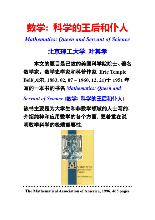
数学: 科学的王后和仆人Mathematics: Queen and Servant of Science北京理工大学叶其孝本文的题目是已故的美国科学院院士、著名数学家、数学史学家和科普作家Eric Temple Bell(贝尔, 1883, 02, 07 ~ 1960, 12, 21)于1951年写的一本书的书名Mathematics: Queen and Servant of Science (数学: 科学的王后和仆人). 该书主要是为大学生和非数学领域的人士写的, 介绍纯粹和应用数学的各个方面, 更着重在说明数学科学的极端重要性.The Mathematical Association of America, 1996, 463 pages实际上这是他1931年写的The Queen of the Sciences (科学的王后)和1937年写的The Handmaiden of the Sciences (科学的女仆)这两本通俗数学论著的合一修订扩大版.Eric Temple Bell Alexander Graham Bell (1847 ~ 1922) 按常识的理解, 女王是优美、高雅、无懈可击、至尊至贵的, 在科学中只有纯粹数学才具有这样的特点, 简洁明了的数学定理一经证明就是永恒的真理, 极其优美而且无懈可击;另一方面, 科学和工程的各个分支都在不同程度上大量应用数学, 这时数学科学就是仆人, 这些仆人是否强有力, 用起来是否得心应手是雇佣这些仆人的主人最为关心的事. 事实上, servant这个字本身就有“供人们利用之物, 有用的服务工具”的意思. 毫无疑问, 我们的目的不是为数学争一个好的名分, 而是想说明数学是怎样通过数学建模来解决各种实际问题的; 数学(数学建模)的极端重要性, 以及探讨正确认识和理解数学科学的作用对于发展我国科学技术、经济以及教育, 从而争取在21世纪把我国真正建设成为屹立于世界民族之林的强国，乃至个人事业发展的至关重要性. 当然, 我们也希望说明王后和仆人集于一身并不矛盾. 历史上, 很多特别受人尊敬的科学家, 不仅仅是由于他们的科学成就, 更因为他们的科学成就能够服务于人类.数学是科学的王后, 算术是数学的王后. 她常常放下架子为天文学和其他科学效劳, 但是在所有情况下, 第一位的是她(数学)应尽的责任. (高斯)Mathematics is the Queen of the Sciences, and Arithmetic the Queen of Mathematics. She often condescends to render service to astronomy and other natural sciences, but under all circumstance the first place is her due.— Carl Friedrich Gauss (卡尔·弗里德里希·高斯, 1777, 4, 30 ~ 1855, 2, 23)From: Bell, Eric T., Mathematics: Queen and Servant of Science, MAA, 1951, p.1;Men of Mathematics, Simon and Schuster, New York, 1937, p. xv.***************************************************自古以来，数学的发展始终与科学技术的发展紧密相连，反之亦然. 首先, 我们来看一下导致我们现在这个飞速发展的信息社会的19、20世纪几乎所有重大科学理论的发展和完善过程中数学(数学建模)所起到的不可勿缺的作用.数学研究的成果往往是重大科学发明的催生素(仅就19、20世纪而言, 流体力学、电磁理论、相对论、量子力学、计算机、信息论、控制论、现代经济学、万维网和互联网搜索引擎、生物学、CT、甚至社会政治学领域等). 但是20世纪上半世纪, 数学虽然也直接为工程技术提供一些工具, 但基本方式是间接的: 先促进其他科学的发展, 再由这些科学提供工程原理和设计的基础. 数学是幕后的无名英雄.现在, 数学无处不在, 数学和工程技术之间,在更广阔的范围内和更深刻的程度上, 直接地相互作用着, 极大地推动了科学和工程科学的发展, 也极大地推动了技术的发展. 数学不仅是幕后的无名英雄, 很多方面开始走向“前台”. 但是对数学的极端重要性迄今尚未有共识, 取得共识对加强一个国家的竞争力来说是至关重要的.硬能力―一位美国朋友谈及对未来中国人的看法: 20年后, 中国年轻人会丢了中国人现在的硬能力, 他们崇拜各种明星, 不愿献身科学, 不再以学术研究为荣, 聪明拔尖的学生都去学金融、法律等赚钱的专业; 而美国人因为认识到其硬能力(例如数学)不行, 进行教育改革, 20年后, 不但保持了其软实力即非专业能力的优势, 而且在硬能力上赶上中国人.‖“正在丢失的硬实力”, 鲁鸣, 《青年文摘》2011年第5期动向：美国很多州新办STEM高中, 一些大学开始开设STEM课程等.STEM = Science + Technology + Engineering + Mathematics2012年2月7日公布的美国总统科技顾问委员会给总统的报告，参与超越：培养额外的100万具有科学、技术、工程和数学学位的大学生(Engage to Excel: Producing One Million Additional College Graduates with Degrees in Science, Technology, Engineering, and Mathematics)The Mathematical Sciences in 2025, the National Academies Press, 2013人们使用的数学科学思想、概念和方法的范围在不断扩大的同时，数学科学的用途也在不断扩展. 21世纪的大部分科学与工程将建立在数学科学的基础上.This major expansion in the uses of the mathematical sciences has been paralleled by a broadening in the range of mathematical science ideas and techniques being used. Much of twenty-first century science and engineering is going to be built on a mathematical science foundation, and that foundation must continue to evolve and expand.数学科学是日常生活的几乎每个方面的组成部分.互联网搜索、医疗成像、电脑动画、数值天气预报和其他计算机模拟、所有类型的数字通信、商业和军事中的优化问题以及金融风险的分析——普通公民都从支撑这些应用功能的数学科学的各种进展中获益，这样的例子不胜枚举.The mathematical sciences are part of almost every aspect of everyday life. Internet search, medical imaging, computer animation, numerical weather predictions and othercomputer simulations, digital communications of all types, optimization in business and the military, analyses of financial risks —average citizens all benefit from the mathematical science advances that underpin these capabilities, and the list goes on and on.调查发现:数学科学研究工作正日益成为生物学、医学、社会科学、商业、先进设计、气候、金融、先进材料等许多研究领域不可或缺的重要组成部分. 这种研究工作涉及最广泛意义下数学、统计学和计算综合，以及这些领域与潜在应用领域的相互作用. 所有这些活动对于经济增长、国家竞争力和国家安全都是至关重要的，而且这种事实应该对作为整体的数学科学的资助性质和资助规模产生影响. 数学科学的教育也应该反映数学科学领域的新的状况.Finding: Mathematical sciences work is becoming an increasingly integral and essential component of a growing array of areas of investigation in biology, medicine, social sciences, business, advanced design, climate, finance, advanced materials, and many more. This work involves the integration of mathematics, statistics, and computation in the broadest sense and the interplay of these areas withareas of potential application. All of these activities are crucial to economic growth, national competitiveness, and national security, and this fact should inform both the nature and scale of funding for the mathematical sciences as a whole. Education in the mathematical sciences should also reflect this new stature of the field.****************************************************************为了以下讲述的方便, 我们先来了解一下什么是数学建模.数学模型(Mathematical Model)是用数学符号对一类实际问题或实际发生的现象的(近似的)描述.数学建模(Mathematical Modeling)则是获得该模型并对之求解、验证并得到结论的全过程.数学建模不仅是了解基本规律, 而且从应用的观点来看更重要的是预测和控制所建模的系统的行为的强有力的工具.数学建模是数学用来解决各种实际问题的桥梁.↑→→→→→→→→↓↑↓↑↓↓↑↓←←←←←通不过↓↓通过)定义：数学建模就是上述框图多次执行的过程数学建模的难点观察、分析实际问题, 作出合理的假设, 明确变量和参数, 形成明确的数学问题. 不仅仅是翻译的问题; 涉及的数学问题可能是复杂、困难的, 求解也许涉及深刻的数学方法. 如何作出正确的判断, 寻找合适、简洁的(解析或近似) 解法; 如何验证模型.简言之:合理假设、模型建立、模型求解、解释验证.记住这16个字, 将会终生受用.数学建模的重要作用：源头创新当然数学建模也有局限性, 不能单独包打天下, 因为实际问题是非常复杂的, 需要多学科协同解决.在图灵(A. M. Turing)的文章: The Chemical Basis of Morphogenesis (形态生成的化学基础), Philosophical Transactions of the Royal Society of London (伦敦皇家学会哲学公报), Series B (Biological Sciences),v.237(1952), 37-72.1. 一个胚胎的模型. 成形素本节将描述一个正在生长的胚胎的数学模型. 该模型是一种简化和理想化, 因此是对原问题的篡改. 希望本文论述中保留的一些特征, 就现今的知识状况而言, 是那些最重要的特征.1. A model of the embryo. MorphogensIn this section a mathematical model of the growing embryo will be described. This model will be asimplification and an idealization, and consequently a falsification. It is to be hoped that the features retained for discussion are those of greatest importance in the present state of knowledge.想单靠数学建模本身来解决重大的生物学问题是不可能的，另一方面，想仅仅依靠实验来获得对生物学的合理、完整的理解也是极不可能的. There is no way mathematical modeling can solve major biological problems on its own. On the other hand, it ishighly unlikely that even a reasonably complete understanding could come solely from experiment.—— J. D. Murray, Why Are There No 3-Headed Monsters? Mathematical Modeling in Biology, Notices of the AMS,v. 59 (2012), no. 6, p.793.自古以来公平、公正的竞赛都是培养、选拔人才的重要手段, 科学和数学也不例外.中学生IMO (国际数学奥林匹克(International Mathematical Olympiad), 1959 ～)北美的大学生Putnbam数学竞赛(1938 ～)全国大学生数学竞赛(2010 ～)Mathematical Contest in Modeling (MCM, 1985 ～)美国大学生数学建模竞赛Interdisciplinary Contest in Modeling (ICM, 1999～)美国大学生跨学科建模竞赛China Undergraduate Mathematical Contest in Modeling (CUMCM, 1992～) 中国大学生数学建模竞赛中国大学生参加美国大学生数学建模竞赛情况中国大学生数学建模竞赛情况在以下讲述中涉及物理方面的具体的数学模型 (问题)的叙述和初步讨论可参考《物理学与偏微分方程》, 李大潜、秦铁虎编著, (上册, 1997; 下册, 2000), 高等教育出版社.Seven equations that rule your world (主宰你生活的七个方程式), by Ian Stewart, NewScientist, 13 February 2012.Fourier transformation 2ˆ()()ix f f x e dx πξξ∞--∞=⎰Wave equation 22222u u c t x ∂∂=∂∂ Ma xwell‘s equation110, , 0, H E E E H H c t c t∂∂∇⋅=∇⨯=-∇⋅=∇⨯=∂∂Schrödinger‘s equation ˆψH ψi t∂=∂Ian Stewart, In Pursuit of the Unknown:17 Equations That Changed the World (追求对未知的认识：改变世界的17个方程), Basic Books, March 13, 2012.目录(Contents)Why Equations? /viii1. The squaw on the hippopotamus ——Pythagoras‘sTheorem/12. Shortening the proceedings —— Logarithms/213. Ghosts of departed quantities —— Calculus/354. The system of the world ——Newton‘s Law ofGravity/535. Portent of the ideal world —— The Square Root ofMinus One/736. Much ado about knotting ——Euler‘s Formula forPolyhedra/837. Patterns of chance —— Normal Distribution/1078. Good vibrations —— Wave Equation/1319. Ripples and blips —— Fourier Transform/14910. The ascent of humanity —— Navier-StokesEquation/16511. Wave in the ether ——Maxwell‘s Equations/17912. Law and disorder —— Second Law ofThermodynamics /19513. One thing is absolute —— Relativity/21714. Quantum weirdness —— Schrödinger Equation/24515. Codes, communications, and computers ——Information Theory/26516. The imbalance of nature —— Chaos Theory/28317. The Midas formula —— Black-Scholes Equation/195Where Next?/317Notes/321Illustration Credits/330Index/331相对论Albert Einstein(1879, 3, 14 ～1955, 4, 18)20世纪最伟大的科学成就莫过于Einstein(爱因斯坦)的狭义和广义相对论了, 但是如果没有Minkowski (闵可夫斯基)几何、Riemann(黎曼)于1854年发明的Riemann几何, 以及Cayley(凯莱), Sylvester(西勒维斯特)和Noether(诺特)等数学家发展的不变量理论, Einstein的广义相对论和引力理论就不可能有如此完善的数学表述. Einstein自己也不止一次地说过.早在1905年, 年仅26岁的爱因斯坦就已提出了狭义相对论. 狭义相对论推倒了牛顿力学的质量守恒、能量守恒、质量能量互不相关、时空永恒不变的基本命题. 这是一场真正的科学革命.为了导出狭义相对论，爱因斯坦作出了两个假设：运动的相对性(所有匀速运动都是相对的)和光速为常数(光的运动例外, 它是绝对的). (1)狭义相对性原理,即在所有惯性系中, 物理学定律具有相同的数学表达形式;(2)光速不变原理,真空中光沿各个方向传播的速率都相等，与光源和观察者的运动状态无关.时空不是绝对独立的.由此可以导出一些推论: 相对论坐标变换式和速度变换式, 同时的相对性, 钟慢尺缩效应和质能关系式等.他的好友物理学家P.Ehrenfest指出实际上还蕴涵着第三个假设, 即这两个假设是不矛盾的. 物体运动的相对性和光速的绝对性, 两者之间的相互制约和作用乃是相对论里一切我们不熟悉的时空特征的根源.(部分参阅李新洲:《寻找自然之律--- 20世纪物理学革命》, 上海科技教育出版社, 2001.)1907 年德国数学家H. Minkowski (1864 ～1909) 提出了―Minkowski 空间‖,即把时间和空间融合在一起的四维空间1,3R. Minkowski 几何为Einstein 狭义相对论提供了合适的数学模型.“没有任何客观合理的方法能够把四维连续统分离成三维空间连续统和一维时间连续统. 因此从逻辑上讲, 在四维时空连续统(space- time continuum)中表述自然定律会更令人满意. 相对论在方法上的巨大进步正是建立在这个基础之上的, 这种进步归功于闵可夫斯基(Minkowski).”—Albert Einstein, The Meaning of Relativity, 1922, Princeton University Press. 中译本, 阿尔伯特·爱因斯坦著, 相对论的意义, (普林斯顿科学文库(Princeton Science Library) 1), 郝建纲、刘道军译, 上海科技教育出版社, 2001, p. 27.有了Minkowski 时空模型后, Einstein 又进一步研究引力场理论以建立广义相对论. 1912 年夏他已经概括出新的引力理论的基本物理原理, 但是为了实现广义相对论的目标, 还必须寻求理论的数学结构, Einstein 为此花了 3 年的时间, 最后, 在数学家M. Grossmann 的介绍下学习掌握了发展相对论引力学说所必需的数学工具—以Riemann几何和Ricci, Levi - Civita的绝对微分学, 也就是Einstein 后来所称的张量分析.“根据前面的讨论, 很显然, 如果要表达广义相对论, 就需要对不变量理论以及张量理论加以推广. 这就产生了一个问题, 即要求方程的形式必须对于任意的点变换都是协变的. 在相对论产生以前很久, 数学家们就已经建立了推广的张量演算理论. 黎曼(Riemann)首先把高斯(Gauss)的思路推广到了任意维连续统, 他很有预见性地看到了……进行这种推广的物理意义. 随后, 这个理论以张量微积分的形式得到了发展, 对此里奇(Ricci)和莱维·齐维塔(Tulio Levi-Civita, 1873～1941)做出了重要贡献. ”—阿尔伯特·爱因斯坦著, 相对论的意义, 郝建纲、刘道军译, 上海科技教育出版社, 2001, p. 57.从数学建模的角度看, 广义相对论讨论的中心问题是引力理论, 其基础是以下两个假设: 1. (等效原理)惯性力场与引力场的动力学效应是局部不可分辨的，(或说引力和非惯性系中的惯性力等效)；2. (广义相对性原理) 一切参考系都是平权的，换言之，客观的真实的物理规律应该在任意坐标变换下形式不变——广义协变性(即一切物理定律在所有参考系[无论是惯性的或非惯性的]中都具有相同的形式)。

1、下载文档前请自行甄别文档内容的完整性，平台不提供额外的编辑、内容补充、找答案等附加服务。
2、"仅部分预览"的文档,不可在线预览部分如存在完整性等问题,可反馈申请退款(可完整预览的文档不适用该条件!)。
3、如文档侵犯您的权益，请联系客服反馈,我们会尽快为您处理(人工客服工作时间：9:00-18:30)。

arXiv:hep-th/9803068v3 14 Apr 1998ILL-(TH)-98-01hep-th/9803068

TheLargeNLimitofthe(2,0)SuperconformalFieldTheory

RobertG.Leigh∗†andMosheRozali‡DepartmentofPhysicsUniversityofIllinoisatUrbana-ChampaignUrbana,IL61801

February1,2008

AbstractWediscussthelargeNlimitofthe(2,0)ﬁeldtheoryinsixdimen-sions.WedothisbyassumingthevalidityofMaldacena’sconjectureofthecorrespondencebetweenlargeNgaugetheoriesandsupergrav-itybackgrounds,hereAdS7×S4.Wereviewthespectrumofthesupergravitytheoryandcomputethespectrumofprimaryoperatorsoftheconformalalgebraofarbitraryspin.1IntroductionAninterestingdevelopmentstemmingfrominvestigationsofstringdualityistheexistenceofhigherdimensionalinteractingsuperconformalﬁxedpoints.Thesimplestsuchﬁxedpointisthe(2,0)ﬁeldtheoryinsixdimensions.Thetheorycanbediscoveredontheworld-volumeoftheM-theory5-branes[3],andinthecompactiﬁcationoftypeIIBstringtheoryonasingularK3[2].Thistheory,compactiﬁedona5-torus,isalsorelevanttoMatrixtheory[4]compactiﬁcationsonT4[5,6].TherealizationofthetheoryasembeddedinM-theoryleavesmanyques-tionsopen.Thetheoryofasingleﬁvebraneisafreeﬁeldtheorycontainingonefreetensormultiplet.ForNﬁvebranesoneexpectstogetaninteractingﬁeldtheoryataﬁxedpointoftherenormalizationgroup[11].Onewouldlikethereforetocomputedimensionsofprimaryoperatorsandtheircorrelationfunctionsinordertoextractinformationaboutthetheory.SomeprogresshasbeenmadeinRef.[1],inwhichtheDLCQofthe(2,0)theorywasdiscussed,viatheMatrixdescriptionofM-theory.Severalquantitieswerecomputed,forlowvaluesofN.Recently,Maldacena[7,8]hasmadethesuggestionthatlargeNgaugetheoriesarerelatedtosupergravityonanti-deSitter(AdS)space.1Inthecaseofmaximalsupersymmetry,thefullspaceisAdSn×C,whereCisasphereofappropriatedimension.Thisconjecturehasbeensigniﬁcantlyclariﬁedbytherecentworkof[10].Inthepresentpaper,westudythecaseofsupergravityonAdS7×S4,whichisrelatedtothetheoryoftheM5-brane,andthusshouldgiveinformationonthe(2,0)theoryinthelargeNlimit.Similarstudieshavebeendone[13,14]intheAdS5×S5case,wherethecorrespondinggaugetheoryistherelativelywell-understoodN=4,d=4SU(N)Yang-Millstheory.Inthiscase,however,weexpecttolearnsomethingnewaboutthe(2,0)theory,atleastintheinﬁniteNlimit.Assumingthevalidityoftheconjecture,thereisacorrespondencebetweenthespectrumofmassesontheAdSspaceandthespectrumofdimensionsofoperatorsintheconformalﬁeldtheory[10].Insection2weextendtheanalysisof[10]tonon-scalaroperators.InparticularweﬁndacorrelationbetweenthesignofthemassofafermionicstateonAdS7andthechiralityoftheoperatoritinducesontheboundary.Usingthisanalysisweconstructinsection3thespectrumoftheconformalprimaryoperatorsofarbitraryspininthe(2,0)theory.Accordingtotheconjecturein[7]thisisacompletelistoftheprimaryoperatorswhosedimensionisﬁniteintheinﬁniteNlimit.Afterthisworkwascompleted,wereceivedtwopaperswhichdiscusssimilarissues[19,20].Ourresults,wheretheyoverlap,areinagreement.

2KKModesofd=11SupergravityonS4In[10]aninterpretationofMaldacena’sconjecturewassuggested.ThegaugetheoryisdescribedbythesupergravitybackgroundviaaholographicimageontheboundaryoftheAdSspace.Thereisaone-to-onemappingofbulksupergravitymodesandconformaloperatorsintheboundarytheory.TheKaluza-Kleinmodesonthesphereplayaspecialrole,sincetheydescribethecompletesetofoperatorswhosedimensionsareindependentofNinthelargeNlimit.ItisknownthatallsuchKaluza-KleinmodesappearasshortmultipletsofthesupersymmetryalgebrainanAdSbackground[18].Thescalingdimensionofagivenboundaryoperatorisrelatedtoamassparameterofthecorrespondingbulksolution.Inthissection,wereviewthisrelationandextendittooperatorsofarbitraryspin.TheKaluza-Kleinmodesofd=11supergravityonS4areknown,havingbeenworkedoutinRefs.[16,15].Itshouldthusbeasimpletasktoidentifytheprimaryoperatorsofthed=6superconformaltheory.Theoperators,beingelementsofshortmultiplets,shouldsaturatecertainunitarityboundswhichhaverecentlybeenworkedoutinRef.[12].WewillrefertothebulkasM,andthe6-dimensionalboundaryasB.Wedenoteamodeinthebulkgenericallyasj{α},whereαisacollectionofquantumnumberslabelingtherepresentationofthesuperconformalalgebraSp(6,2|4);itissuﬃcienttogivequantumnumbersofthemaximalcompactsubgroup,hereSpin(5,1)×Spin(2)×Sp(2)R.ThebulkmodecouplestoanoperatorontheboundaryO{¯α},where¯αistheconjugaterepresentation.Forexample,ifjisachiralspinor,thecorrespondingOisananti-chiralspinor;similarlyifjisaself-dualtensor,thenOisanti-self-dual.Thecouplingissimplyoftheform󰀃

Bj{α}·O{¯α}(1)