《金融工程》案例解析(英文版)
清华大学金融工程学10

? 浮动利率短期证券( FIRSTS);
? 不发达国家( LDC)债转股融资;
? 可分拆股票组合单位( USUs,没有推出)
金融工程案例分析
5
USUs产品
USU(Unbundled Stock Units)
? 一种交换权,股东有权以普通股交换一个包含 债券、优先股和股票认购证的证券组合。
? USU产品的特点:
金融工程案例分析
共同的原 因
作为 covered warrant, 法律上认 为是证券, 而不是期 权
17
案例简要回顾
? SLH的分析人员注意到近来欧洲市场的一 批新产品交易——合成担保认股权证 (Synthetic Covered Warrants )。这种认 股权证由银行家信托公司(BT)于1989年 4月首次在欧洲市场上发行,本质上属于 对美国蓝筹股的长期看涨期权。
金融工程案例分析
14
三种covered warrants
发行者 标的物
有否保证
Back-to-back warrant
Stillhalter
银行 银行
Synthetic covered 银行 warrant
日本公司的 认股权证
该银行股东 的股票
美国蓝筹公 司的股票
有 (认股权证) 有 (股票)
无,可认为 是信用担保
? 绑定发售; ? 组合可分拆进行交易
金融工程案例分析
6
USUs产品
? 已有4家蓝筹公司,公开宣布愿意发行56 亿美元的USU产品:
? 美国运通; ? 道氏化学公司; ? 辉瑞; ? Sara Lee
? “USU将s 成为90年代的金融狂热”
——Business Week评论
金融工程英文
AbstractPurpose –The purpose of this paper is to provide a general discussion of how techniques from financial engineering can be used to investigate the economic costs of farm programs and to aid in the design of new financial products to implement margin protection for dairy farmers. Specifically the paper investigates the Milk Income Loss Contract (MILC) and the Dairy Margin Protection (DMP) program. In addition the paper introduces the concept of the Milk to Corn Price ratio to protect margins.Design/methodology/approach –The paper introduces and reviews the tools of financial engineering. These include the stochastic calculus and Itoˆ’s Lemma. The empirical tool is Monte Carlosimulations. The approach is part pedagogy and part practice.Findings –In this paper the authors illustrate how financial engineering can be used to price complex price stabilization formula in the USA and to illustrate its use in the design of new products. Practical implications –In this paper the authors illustrate how financial engineering can be used to price complex price stabilization formula in the USA and to illustrate its use in the design of new products.Social implications–Farm programs designed to protect dairy farmers margins are designed in a seemingly ad hoc fashion. Assessments of programs such as MILC or DMP are conducted on an ex-post basis using historical data. The financial engineering approach presented in this paper provides the means to add significant depth to the assessment of such programs which can be used in conjunction with Monte Carlo simulation to identify alternative model structures before they are written into law.Originality/value –This paper builds upon an existing literature. Its originality is in the application of financial engineering techniques to farm dairy policy.Keywords :Dairy policy, DMP, Financial Engineering, Itoˆ’s lemma, MILC, Milk to corn ratio Agricultural policy in the USA and elsewhere has from time to time established programs that in one form or another have been structured around the randomness of prices with the objective of providing some form of stabilization. These have included loan rates and target prices under the Commodity Credit Corporation until 2002 and currently revolving around flex payments, direct and countercyclical payments, SURE (the Supplemental Revenue Assistance Program), ACRE (Average Crop Revenue Election) and for dairy the Milk Income Loss Contract (MILC) in the 2008 Farm Bill (Bekkerman et al, 2012). In addition to these, new programs have evolved on a revenue basis with insurance indemnities paid on the joint outcomes of crop yield and market prices. Indeed, it seems that any new Farm Bill has some evolutionary or revolutionary stabilization program as part of its text, and sometimes in a rather convoluted and seemingly ad hoc form. For example, a host of volumetric or revenue-based programs are proposed in the 2013 Farm Bill including ARC (Agricultural Risk Coverage), STAX (the Stacked Income Protection Plan), RLC (Revenue Loss Coverage) and SCO (The Supplemental Coverage Option) (Paulson et al., 2013; Barut and Collins, 2014).Since the 1970s there has been a general interest in determining the value of a particular program both in terms of welfare to farmers and public expenditure to the tax payers (Marcus and Modest, 1986; Brinch and Stokes, 2001; Hertzler, 1991; Pederson and Zhou, 2009; Richards and Manfredo, 2003; Stokes and Nayda, 2003; Stokes et al., 1997; Tirupattur et al., 1997; Turvey et al., 1988; Turvey, 1992; Turvey and Stokes, 2008; Yin and Turvey, 2003). But while this interest is alwaysthere, the actual practice of determining program value has been limited in application. The traditional approach to valuing agricultural policy programs has relied heavily on demand and supply side interactions to generate price changes. However, in practice, price dynamics of both inputs and outputs are subject to significant variation that is persistent, volatile and unexplained by equilibrium models. Financial engineering uses stochastic calculus to directly model price dynamics and the underlying risks embedded in the farm problem.In this paper we explore financial engineering as a mechanism for understanding the farm problem in a number of contexts. First we introduce the idea of financial engineering through a primer on the stochastic calculus or Itoˆ’s Lemma (Itoˆ, 1942a, b, 1944a, b, 1951a, b; Jarrow and Protter, 2004; McKean 2007). Then we show how contingent claims policies such as MILC and Dairy Margin Protection (DMP) with non-linear payoffs to farmers can be priced or valued using financial engineering techniques similar to the pricing of conventional options in a Black and Scholes (1973) framework. We also illustrate how new risk management products can be financially engineered. In particular, we apply financial engineering techniques to the milk to corn price ratio and provide some preliminary evidence on the effectiveness of the new risk management product in hedging milk revenue margins.Dairy producers confront various sources of risk. Among those, the uncertainty associated with the future cash price of a commodity is known as price risk. Theincrease in the price volatility of milk, corn and soybean in recent years[1] poses an increasing threat to the business survival of dairy producers. In New York State all-milk prices have not increased much for the past 15 years[2] while corn and soybean prices have soared since 2006. While the rising feed costs may be temporary, if dairy farmers in New York are inadequately hedged against this risk, shrinking profit margins may lead them to the brink of bankruptcy. Consequently, dairy farm profits are not only affected by the price risk from the milk price received, but also by the volatility in input prices. Dairy feed, which mainly consists of corn, hay and soybean, is one of the most important inputs for dairy producers. As a non-storable commodity, there could be large swings in milk prices in reaction to changes in market fundamentals. On the other hand, increasing costs and highly volatile feed prices further threaten the survival of dairy farm businesses.It is not surprising then that dairy policy focusses not on the price of the output, per se, but on protecting the margin, or spread, between market-driven prices (revenues) and feed costs. While there have been ample papers written on various aspects of dairy policy, it is surprising that few papers recognize the broader aspect of financial engineering to resolve the farm problem. In this paper we show how stochastic calculus can be used directly on simulated price processes to value not only milk stabilization policies, but to develop new products to solve the farm problem.The overarching goal of this paper is to “illustrate”the basic application of the stochastic calculus to the farm problem. It is intentionally part pedagogy. In the following section we provide a primer on Itoˆ’s Lemma and the stochastic calculus –the workhorse of financial engineers –and illustrate their use in a general setting. We then investigate with greater depth the application of financial engineering to the farm problem. Specifically we show how the MILC and DMP programs can be captured by a simple stochastic process that can be used as the basis of Monte Carlo simulations for “pricing”the imbedded options in these programs. In additionwe propose a new futures/options contracts based on the Class III milk/corn ratio for the explicit purpose of protecting profit margin for dairy producers with only one hedge position in the market. We illustrate how an option on this milk/corn price ratio can be computed using the Black-Scholesmodel as well as by Monte Carlo techniques. We then illustrate how these “options”can be priced using Monte Carlo techniques and conclude the paper.。
金融工程名词解释英文版
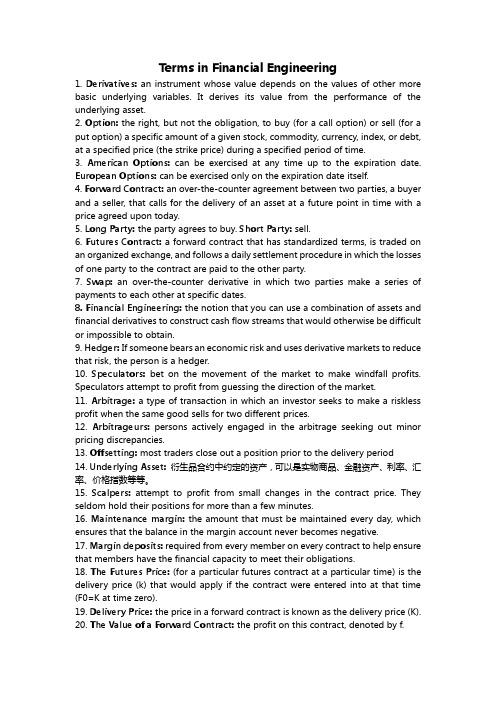
Terms in Financial Engineering1. Derivatives: an instrument whose value depends on the values of other more basic underlying variables. It derives its value from the performance of the underlying asset.2. Option: the right, but not the obligation, to buy (for a call option) or sell (for a put option) a specific amount of a given stock, commodity, currency, index, or debt, at a specified price (the strike price) during a specified period of time.3. American Options: can be exercised at any time up to the expiration date. European Options: can be exercised only on the expiration date itself.4. Forward Contract: an over-the-counter agreement between two parties, a buyer and a seller, that calls for the delivery of an asset at a future point in time with a price agreed upon today.5. Long Party: the party agrees to buy. Short Party: sell.6. Futures Contract: a forward contract that has standardized terms, is traded on an organized exchange, and follows a daily settlement procedure in which the losses of one party to the contract are paid to the other party.7. Swap: an over-the-counter derivative in which two parties make a series of payments to each other at specific dates.8. Financial Engineering: the notion that you can use a combination of assets and financial derivatives to construct cash flow streams that would otherwise be difficult or impossible to obtain.9. Hedger: If someone bears an economic risk and uses derivative markets to reduce that risk, the person is a hedger.10. Speculators: bet on the movement of the market to make windfall profits. Speculators attempt to profit from guessing the direction of the market.11. Arbitrage: a type of transaction in which an investor seeks to make a riskless profit when the same good sells for two different prices.12. Arbitrageurs: persons actively engaged in the arbitrage seeking out minor pricing discrepancies.13. Offsetting: most traders close out a position prior to the delivery period14. Underlying Asset: 衍生品合约中约定的资产,可以是实物商品、金融资产、利率、汇率、价格指数等等。
Ch11_The Black-Scholes Model(金融工程-华东师范大学 汤银才)解读
11.7
The Expected Return
The expected value of the stock price is E(ST)=S0emT The expected continuously compounded return on the stock is E()=m – 2/2 (the geometric average) m is the the arithmetic average of the returns Note that E[ln(ST)] is not equal to ln[E(ST)]
11.1
The Black-Scholes Model
Chapter 11
Options, Futures, and Other Derivatives, 4th edition © 2000 by John C. Hull Tang Yincai, © 2003, Shanghai Normal University
However, the geometric average is
n g (1 xi ) i 1
1 n
_
n
i 1
1 (1.10 * 1.12 * 1.08 * 1.09 * 1.11
11.8
The Expected Return Example
Take the following 5 annual returns: 10%, 12%, 8%, 9%, and 11% The arithmetic average is
x 1 n xi 15 (0.10 0.12 0.08 0.09 0.11) 15 * 0.50 0.10
金融工程学导论英文版
Lesson- 1: Introduction to financial engineeringObjectivesUpon completion of this lesson you will be able toExplain the nature and scope of financial engineeringIdentify the objectives of financial engineeringDiscuss the importance and limitations of financial engineeringGood Morning/ afternoon / evening to all.This is the first session with you in this subject. With good gesture we will start this subject and I really expect from your side a lot of contribution otherwise you may not be able to understand this subject thoroughly.I would like to convey you – this subject is highly mathematical. You will apply all your mathematical and quantitative techniques knowledge in the financial theories, economic models and financial decisions taking. All these concepts, you have to recall very nicely before you proceed for this subject. Anyway its fine we all are in good spirit to proceed. Okay?In a very simple term financial engineering is the process by which a portfolio is designed and maintained in such a manner as to achieve specified goals. Financial institutions use financial engineering to create complex derivative instruments.Anyway this lesson introduces some simple financial engineering strategies. We consider two examples that require finding financial engineering solutions to a daily problem. In each case, solving the problem under consideration requires creating appropriate synthetics. In doing so legal, institutional and regulatory issues need to be considered.The nature of the examples themselves is secondary here. Our main purpose is to bring to the forefront the way of solving problems using financial securities and their derivatives. The lesson does not go into the details of the terminology or of the tools that are used. In fact, some of you may not even be able to follow the discussion fully. There is no harm in this since these will be explained in later lessons.Let’s say about a money market ProblemConsider a Japanese bank in search of a 3-month money market loan. The bank would like to borrow U.S. dollars (USD) in Euromarkets and then on-lend them to its customers. This interbank loan will lead to cash flows as shown in Figure I-I. From the borrower's angle USD 100 is received at time to and then it is paid back with interest 3 months later at time t0 + δ. The interest rate is denoted by the symbol L to¼ and is determined at time t0. The tenor of the loan is 3 months. Thereforeδ = 14and the interest paid becomes L to ¼. The possibility of default is assumed away.Otherwise at time t0 + δ there would be a conditional cash flow depending on whether or not there is default.The money market loan displayed here is a fairly liquid instrument. In fact, banks purchase such "funds" in the wholesale interbank markets and then on-lend them to their customers at a slightly higher rate of interest.Now you see the ProblemSuppose the above mentioned Japanese bank finds out that this loan is not available due to the lack of appropriate credit lines. The counterparties are unwilling to extend the USD funds. The question then is: Are there other ways in which such dollar funding can be secured?The answer is yes. In fact, the bank can use foreign currency markets judiciously to construct exactly the same cash flow diagram as in Figure 1-1 and thus create a synthetic money market loan. This may seem an innocuous statement, but note that using currency markets and their derivatives will involve a completely different set of financial contracts, players, and institutional setup than the money markets. Yet, the result will be cash flows identical to those in Figure 1-1.We can come to the solution as:To see how a synthetic loan can be created, consider the following series of operations:1. The Japanese bank first borrows local funds in yen in the Japanese money markets. This is shown in the Figure. The bank receives yen at time t0 and will pay yen interest rate L y to.2. Next, the bank sells these yen in the spot market at the current exchange rate e to to secure USD 100. This spot operation is shown in the coming Figure.3. Finally, the bank must eliminate the currency mismatch introduced by these operations: In order to do this, the Japanese bank buys 100(1 + L toδ)f to yen at the known forward exchange rate fto' in the forward currency markets. This is the cash flow shown in the third Figure that follows. Here, there is no exchange of funds at time to. Instead, forward dollars will be exchanged for forward yen at t0 + δ.Now comes the critical point. In Figure two, add vertically all the cash flows generated by these operations. The yen cash flows will cancel out at time to because theyare of equal size and different sign. The time t0+ δyen cash flows will also cancel out because that is how the size of the forward contract is selected. The bank purchases just enough forward yen to pay back the local yen loan and the associated interest. The cash flows that are left are shown in fourth Figure and these are exactly the same cash flows as in Figure one. Thus, the three operations have created a synthetic USD loan.Here I would like to share with you some important ImplicationsThere are some subtle but important differences between the actual loan and the synthetic. First, note that from the point of view of euromarket banks, lending to Japanese banks involves a principal of USD 100, and this creates a credit risk. In case of default, the 100 dollars lent may not be repaid. Against this, some capital has to be put aside.Depending on the rate of money markets and depending on counterparty credit risks, money center banks may adjust their credit, lines toward such customers. .In contrast, in the case of the synthetic dollar loan, the international bank's exposure to the Japanese bank is in the forward currency market only. Here, there is no principal involved. If the Japanese bank defaults, the burden of default will be on the domestic banking system in Japan. There is a risk due to the forward currency operation, but it is a coul1terparty risk and is limited. Thus, the Japanese bank may end up getting the desired funds somewhat easier if a synthetic is used. .There is a second interesting point to the issue of credit risk mentioned earlier. The original money market loan was a Euromarket instrument. Banking operations in Euromarkets are considered offshore operations, taking place essentially outside the jurisdiction of national banking authorities. The local yen loan, on the other hand, is obtained in the onshore market. It would be subject to supervision by Japanese authorities. In ease of default, there may be some help from the Japanese Central Bank, unlike a Eurodollar loan where a default may have more severe implications on the lending bank.The third point has to do with pricing. If the actual and synthetic loans have identical cash flows, their values should also be the same excluding credit risk issues. Since, if there is a value discrepancy the markets will simultaneously sell the expensive one, and buy the cheaper one, realizing a windfall gain. This means that synthetics can also be used in pricing the original instrument. 2Fourth, note that the money market loan and the synthetic can in fact be each other's-hedge. Finally, in spite of the identical nature of the involved cash flows, the two ways of securing dollar funding happen in completely different markets and involve very different financial contracts. This means that legal and regulatory differences may be significant.Again let’s relate it to an Example of Taxation.Now consider a totally different problem. We create synthetic instruments to restructure taxable gains. The legal environment surrounding taxation being a complex and ever-changing phenomenon, this example should be read only from a financial engineering perspective and not as a tax strategy. Yet the example illustrates the close connection between what a financial engineer does and the legal and regulatory issues that surround this activity.The Problem Is:In taxation of financial gains and losses, there is a concept known as a wash-sale. Suppose that during the year 2002; an investor realizes some financial gains. Normally, these gains are taxable that year. But a variety of financial strategies can possibly be used to postpone taxation to the year after: To prevent such strategies, national tax authorities have a set of rules known as washsale, and stra4dle rules. It is important that professionals working for national tax authorities in various countries understand these strategies well and have a good knowledge of financial engineering. Otherwise some players may rearrange their portfolios, and this may lead to significant losses in tax revenues. From our perspective, we are concerned with the methodology of constructing synthetic instruments. This example will illustrate another such construction.Suppose that in September 2002, an investor bought an asset at a price So = $100. In December 2002, this asset is sold at S1 = $150. Thus, the investor has realized a capital gain of $50. These cash flows are shown in Figure 1-3. The first cash flow is negative and is placed below the time axis because it is a payment by the investor. The subsequent sale of the asset, on the other hand, is a receipt, and hence is represented by a positive cash flow placed above the time axis. The investor may have to pay significant taxes on these capital gains. A relevant question is then: Is it possible to use a strategy that postpones the investment gain to the next tax year?One may propose the following solution, however, is not permitted under the wash-sale rules. This investor is probably holding assets other than the S t mentioned earlier.After all, the right way to invest is to have diversifiable portfolios. It is also reasonable to assume that if there were appreciating assets such as S t, there were also assets that lost value during the same period. Denote the price of such an asset by Z t. Let the purchase price be Z0. If there were no wash-sale rules, the following strategy could be put together to postpone year 2002 taxes.Sell the Z-asset on December 2002, at a price Z1, Z l< Z0, and. the next day, buy the same Z t at a similar price. The sale will result in a loss equal toZ1 – Z0 < 0(2)The subsequent purchase puts this asset back into the portfolio so that the diversified portfolio can be maintained. This way, the losses in Z t are recognized and will cancel out some or all of the capital gains earned from S t. There may be several problems with this strategy, but one is fatal. Tax authorities would call this a wash-sale (i.e. a sale, that is being’. intentionally used to "wash" the 2002 capital gains) and would disallow the deductions.Another StrategyYet investors can find a way to sell the Z-asset without having to sell it in the usual way. This can be done by first creating a synthetic Z-asset and then realizing the implicit capital losses using this synthetic, instead of the Z-asset held in the portfolio. .Suppose the investor originally purchased the Z-asset at a price Z0= $100 and that' asset is currently trading at Z l = $50, with a paper loss of $50. The investor would like to recognize the loss without directly selling this asset. At the same time the investor would like to retain the original position in the Z-asset in order to maintain a well-balanced portfolio. How can the loss be realized while maintaining the Z-position and without selling the Z t ?The idea is to construct a proper synthetic. Consider the following sequence of operations:• Buy another Z-asset at price Z l = $50 on November 26, 2002. .• Sell an at-the-money call on Z with expiration date December 30, 2002.• Buy an at-the-money put on Z with the same expiration.The specifics of call and put options will be discussed in later chapters. For those readers' with no background in financial instruments we can add a few words. Briefly, options are instruments that give the purchaser a right. In the case of the call option, it is the right to purchase the underlying asset (here the Z-asset) at a pre-specified price (here $50). The put option is the opposite. It is the right to sell the asset at a pre-specified price (here $50). When one sells options, on the other hand, the seller has the obligation to deliver or accept delivery of the underlying at a pre-specified price.For our purposes, what is important is that short call and long put are two securities whose expiration payoff, when added will give the synthetic short position shown in Figure 1-4. By selling the call the investor has the obligation to deliver the Z-asset at a price of $50 if the call holder demands it. The put, on the other hand, gives the investor the right to sell the 2 -asset at $50 if he or she chooses to do so.The important point here is this: When the short call and the long put positions shown in Figure 1 -4 are added together the result will be equivalent to a short position on stock Z t. In fact, the investor has created a synthetic short position using options.Now consider what happens as time passes. If Z t appreciates by December 30, the call will be exercised. This is shown in Figure 1 -5a. The call position will lose money, since the investor has to deliver, at a loss, the original & Z stock that cost $100. If, on the other hand, the Z t decreases, then the put position will enable the investor to sell the original Z -stock at $50. This time the call will expire worthless.3 This situation is shown in Figure l-5b. Again, there will be a loss of $50. Thus, no matter what happens to the price Z t, either the investor will deliver the original Z-asset purchased at a price $100, or the put will be exercised and the investor will sell the original Z-asset at $50. Thus, one way or another, the investor is using the original asset purchased at $ 100 to close an option position at a loss. This means he or she will lose $50 while keeping the same & -position, since the second &, purchased at $50, will still be in the portfolio.The timing issue is important here. For example according to U.S. tax legislation, wash-sale rules will apply if the investor has acquired or sold a substantially identical property within a 3 I -day period. According to the strategy outlined here the second Z is purchased on November 26, while the options expire on December 30. Thus, there are more than 31 days between the two operations.ImplicationThere are at least three interesting points to our discussion. First, the strategy offered to the investor was risk-free and had zero cost aside from commissions and fees. Whatever happens to the new long position in the Z-asset, it will be canceled by the synthetic short position. This situation is shown in the lower half of Figure 1-4. As this graph shows, the proposed solution is risk less. The second point is that, once again, we have created a synthetic, and then used it in providing a solution to the tax problem. Finally, the example displays the crucial role legal and regulatory frameworks can play in devising financial strategies. Although this book does not deal with these issues, it is important to understand the crucial role they play at almost every level of financial engineering.Some Caveats for what is to follow for your proper understandingA newcomer to financial engineering usually follows instincts that are harmful for good understanding of the basic methodologies in the field. Hence, before we start, we need to layout some basic rules of the game that should be remembered throughout the book.1. This book is written from a market practitioner's point of view. Investors, pension funds, insurance companies, and governments are clients, and for us they are always on the other side of the deal. In other words, we look at financial engineering from a trader's, broker's and dealer's angle. The approach is from the manufacturer's perspective rather than the viewpoint of the user of the service. This premise is crucial in understanding some of the logic discussed in later chapters.2. We adopt the convention that there are two prices for every instrument unless stated otherwise. The agents involved in the deals often quote two-way prices. In economic theory, economic agents face the law of one price. The same good or asset cannot have two prices. If it did, we would then buy at the cheaper price and sell at the higher price.Yet in financial markets, there are two prices: one-price at which the financial market participant is willing to buy something from you, and another one at which the financial market participant is willing to sell the same thing to you. Clearly, the two cannot be the same. An automobile dealer will buy a used car at a low price in order to sell it at a higher price. That is how the dealer makes money. The same is true for a financial market practitioner. A swap dealer will be willing 10 buy swaps at a low price in order to sell them' at a higher price later. In the meantime, the instrument will be kept in the inventories, just like the used car sold to a car dealer. .3. A financial market participant is not an investor and never has "money." He or she has to secure funding for any purchase and has to place the cash generated by any sale. In. this book, almost no financial market operation begins with a pile of cash. The only "cash" is in the investor's hands, which in this book is on the other side of the transaction.It is for this reason that market practitioners prefer to work with instruments that have zero-value at the time of initiation. Such instruments would not require funding and are more practical to uses. They also are likely to have more liquidity.4. The role played by regulators professional organizations, and the legal profession is muchmore important for a market professional is much more important for an investor.Although it is far beyond the scope of this book, many financial engineering strategies have been devised for the sole purpose of dealing with them.Remembering these premises will greatly facilitate the understanding of financial engineering.。
Chap014Bond Prices and Yields金融工程英文(王小麓)
Copyright © 2001 by The McGraw-Hill Companies, Inc. All rights reserved.
14-14
Holding-Period Example
CR = 8%
YTM = 8%
N=10 years
Semiannual Compounding P0 = $1000
14-1
Chapter 14
Bond Prices and Yields
McGraw-Hill/Irwin
Copyright © 2001 by The McGraw-Hill Companies, Inc. All rights reserved.
14-2
Bond Characteristics
14-3
Different Issuers of Bonds
U.S. Treasury - Notes and Bonds Corporations Municipalities International Governments and Corporations Innovative Bonds - Indexed Bonds - Floaters and Reverse Floaters
- Future Value: sales price + future value of coupons - Investment: purchase price
McGraw-Hill/Irwin
Copyright © 2001 by The McGraw-Hill Companies, Inc. All rights reserved.
McGraw-Hill/Irwin
Chap024Portfolio Performance Evaluation金融工程英文(王小麓)
Past Performance - generally the geometric mean is preferable to arithmetic
Predicting Future Returns- generally the arithmetic average is preferable to geometric
Complicated subject Theoretically correct measures are difficult to construct Different statistics or measures are appropriate for different types of investment decisions or portfolios Many industry and academic measures are different The nature of active management leads to measurement problems
- Sectors or industries
- Individual companies
McGraw-Hill/Irwin
Copyright © 2001 by The McGraw-Hill Companies, Inc. All rights reserved.
24-11
Risk Adjusted Performance: Sharpe
rp = Average return on the portfolio
rf = Average risk free rate ß p = Weighted average for portfolio
金融工程案例分析
一、案例背景2008 年10 月20 日,中信集团旗下的中信泰富召开新闻发布会。
中信集团主席荣智健表示,由于中信泰富的财务董事越权与香港数家银行签订了金额巨大的澳元杠杆式远期合约导致已经产生8 亿港元的损失,他说,如果以目前的汇率市价估计,这次外汇杠杆交易可能带来高达147 亿港元的损失。
中信泰富的公告表示,有关外汇合同的签订并没有经过恰当的审批,其潜在风险也没有得到评估,因此已终止了部分合约,剩余的合同主要以澳元为主.管理层表示,会考虑以三种方案处理手头未结清的外汇杠杆合同,包括平仓、重组合约等多种手段.荣智健在发布会上称该事件中集团财务总监没有尽到应尽的职责.他同时宣布,财务董事张立宪及财务总监周志贤已提请辞职,并获董事会接受,而与事件相关的人员将会受到纪律处分。
自即日起,中信集团将委任莫伟龙为财务董事。
由于这笔合约的期限为二年,荣智健说如果以目前的汇率市价估计,这次外汇杠杆交易可能带来高达147 亿港元的损失。
中信泰富在澳大利亚有SINO—IRON铁矿投资项目,亦是西澳最大的磁铁矿项目.整个投资项目的资本开支, 除目前的l6亿澳元之外,在项目进行的25年期内,还将至少每年投入10亿澳元,很多设备和投人都必须以澳元来支付。
为降低澳元升值的风险,公司于2008年7月与13家银行共签订了24款外汇累计期权合约,对冲澳元、欧元及人民币升值影响,其中澳元合约占绝大部分。
由于合约只考虑对冲相关外币升值影响,没有考虑相关外币的贬值可能,在全球金融危机迫使澳大利亚减息并引发澳元下跌情况下,2008年10月20日中信泰富公告因澳元贬值跌破锁定汇价,澳元累计认购期权合约公允价值损失约147亿港元;11月14日中信泰富发布公告,称中信集团将提供总额为15亿美元(约ll6亿港元)的备用信贷,用于重组外汇衍生品合同的部分债务义务,中信泰富将发行等值的可换股债券,用来替换上述备用信贷.据香港《文汇报》报道, 随着澳元持续贬值,中信泰富因外汇累计期权已亏损186亿港元.截至2008年12月5日,中信泰富股价收于5.80港元,在一个多月内市值缩水超过2l0亿港元.另外,就中信泰富投资外汇造成重大亏损,并涉嫌信息披露延迟,香港证监会正对其展开调查。
- 1、下载文档前请自行甄别文档内容的完整性,平台不提供额外的编辑、内容补充、找答案等附加服务。
- 2、"仅部分预览"的文档,不可在线预览部分如存在完整性等问题,可反馈申请退款(可完整预览的文档不适用该条件!)。
- 3、如文档侵犯您的权益,请联系客服反馈,我们会尽快为您处理(人工客服工作时间:9:00-18:30)。
Thus, KKR offered common shareholders a 41% premium over the firm’s pre-takeover value.
– $1.0 billion of 15-percent payment-in-kind subordinated debentures due 2001 (pay-in-kind bond)
– $4.1 billion of subordinated discount debentures due 2001 (deferred-coupon bond)
Through acquisitions in the 1960s, the tobacco firm entered a variety of food businesses.
After its 1985 merger, the firm was renamed RJR Nabisco.
返回目录 5
返回目录 8
Financial Engineering
Part Two: Description of Securities
返回目录 9
Financial Engineering
Issuance
In May 1989, RJR holdings Capital Corporation issued three nearly identical debt securities in connection with the leveraged buyout of RJR Nabisco by KKR
– $525 million of 13.5-percent subordinated debentures due 2001 (cash-paying bond)
返回目录 10
Financial Engineering
返回目录 11
Financial Engineering
返回目录 12
Financial Engineering
返回目录 3
Financial Engineering
Part One: Background
返回目录 4
Financial Engineering
Background 1
The firm known in 1991 as RJR Nabisco was a descendant of the tobacco firm R.J. Reynolds, founded in 1875.
返回目录 2
Financial Engineering
Reference:
Robert M. Dammon, Kenneth B. Dunn. And Chester S. Pratt. 1993. The Relative Pricing of High-Yield Debt: The Case of RJR Nabisco Holdings Capital Corporation. the American Economic Review, 83 ( Dec.)
Financial Engineering
Cases in Financialen Miaoxin
返回目录 1
Financial Engineering
The Case of RJR
Nabisco Holding Capital Corporation
– The Management Group
– Kohlberg, Kravis, Roberts &Co. (KKR), a firm specializing in leveraged buyouts
返回目录 6
Financial Engineering
Background 3
At the end of a bidding war, KKR prevailed by offering shareholders $81 per share in cash plus a package of bonds valued at $28.
Financial Engineering
Background 2
In the late 1980s the food products industry experienced massive consolidation through mergers.
In 1988 two main bidders proposed to take the RJR Nabisco private in a leveraged buyout contest:
Each of these related entities had separate obligations, issued either in conjunction with the acquisition or, in the case of RJR Nabisco, Inc, the operating company, carried over from the taken-over firm.
Difference
The major difference among the three securities is the form in which interest is paid.
To finance the buyout, KKR increased RJR’s debt from $5 billion to $29 billion.
返回目录 7
Financial Engineering
Background 4
The new firm was structured as a series of holding companies.