2wln2之3idiots
新视野大学英语第二册Unit3单词
|<1>charactern. 1.性格,个性What does her handwriting tell you about her character? |根据她写的字,你觉得她有什么样的性格?I choose my friends for their good characters. 我择友的标准是品格一定要好。
2. [C]特点,特征The whole character of the village has changed since I was last here. |自我上次来这里之后,这个村子的面貌完全变了。
The idea was to rebuild the house without changing its basic character. |计划是将那幢房子按原貌加以改建。
<2>compromisen. 妥协;折中She found that compromise was always the best way when she quarreled with her mother. |她发现,与母亲争吵时让步总是最好的解决方法。
It is hoped that a compromise will be reached in today's talk. |希望今天的会谈能达成妥协。
v. 妥协;折中The workers are going to strike for their welfare if theemployers are not ready to compromise. |雇主们要是不妥协,工人们就将为争取自己的福利而罢工。
Well, you want $400 and I say $300, so let's compromise at $350. |好吧,既然你开价400美元而我还价300美元,那我们就来个折衷价350美元。
3G手机缩略语
3G手机缩略语.txt单身很痛苦,单身久了更痛苦,前几天我看见一头母猪,都觉得它眉清目秀的什么叫残忍?是男人,我就打断他三条腿;是公狗,我就打断它五条腿! 2G 2nd Generation Mobile Communications System 第二代移动通信系统3G,3GMS 3rd Generation Mobile Communications System 第三代移动通信系统3GPP 3rd Generation Partnership Project 第三代合作组织AAAA Authentication, Authorization, Accounting 鉴权、授权、计费AAL1 ATM Adaptation Layer type 1 ATM适配层类型1AAL2 ATM Adaptation Layer type 2 ATM适配层类型2AAL5 ATM Adaptation Layer type 5 ATM适配层类型5ABR Available Bit Rate 可用比特率ACL Access Control List 访问控制列表ACS Add, Compare, Select 加,比,选ADMF Administration Function at the LIAN LIAN中的管理功能实体ADT Adaptive Dynamic Threshold 自适应动态阀值AG Access Gateway 接入网关AI Acquisition Indicatior 捕获指示AICH Acquisition Indication Channel 捕获指示信道ALIM ATM Line Interface Module subrack ATM线路接口插框AM Account Management 计费管理AM Acknowledged Mode 确认模式AMR Adaptive MultiRate 自适应多速率ANSI American National Standard Institute 美国国家标准组织AoCC Advice of Charge Charging 计费费用通知AoCI Advice of Charge Information 计费信息通知AP Access Point 接入点AP Access Preamble 接入前导APN Access Point Name 接入点名称ARP Address Resolution Protocol 地址解析协议ARQ Automatic Repeat Request 自动重发请求AS Application Server 应用服务器AS Access Stratum 接入层ASC Access Service Class 接入服务类ASCII American Standard Code for Information Interchange 美国信息交换标准码ASF Application Server Function 应用服务器功能ASIC Application Specific Integrated Circuit 专用集成电路ASN.1 Abstract Syntax Notation One 抽象语法编码1ASP Application Server Process 应用服务器进程ASP Access Service Provider 接入服务提供商ATM Asynchronous Transfer Mode 异步传输模式AuC Authentication Center 鉴权中心BBAIC Barring of All Incoming Calls 限制所有入呼叫BAIC-Roam Barring of All Incoming Calls when Roaming outside the home PLMN country当漫游出归属PLMN国家后,限制入呼叫BAM Back Administration Module 后管理模块BAOC Barring of All Outgoing Calls 限制所有出局呼叫BAS Broadband Access Server 宽带接入服务器BC Billing Center 计费中心BCCH Broadcast Control Channel 广播控制信道BCH Broadcast Channel 广播信道BCFE Broadcast Control Functional Entity 广播控制功能实体BER Bit Error Rate 误比特率BGP Border Gateway Protocol 边界网关协议BHCA Busy Hour Calling Attempt 忙时试呼次数BICC Bearer Independent Call Control 承载无关呼叫控制BIOS Basic Input Output System 基本输入输出系统BITS Building Integrated Timing Supply System 通信楼综合定时供给系统BLER Block Error Rate 误块率BMC Broadcast/Multicast Control 广播/组播控制BNET Broadband NETwork subrack 宽带交换网插框BOIC Barring of Outgoing International Calls supplementary service 禁止国际出局呼叫补充业务BOIC-exHC Barring of Outgoing International Calls except those directed to the Home PLMN Country 限制所有除归属国外的国际出局呼叫BOM Bill of Material 物料清单BS Billing System 计费系统BSC Base Station Controller 基站控制器BSP Board Support Packet 板级支持软件包BSS Base Station Subsystem 基站子系统BSSAP Base Station Subsystem Application Part 基站子系统应用部分BTS Base Transceiver Station 基站收发信台CCA Capacity Allocation 容量分配CAA Capacity Allocation Acknowledgement 容量分配确认CAMEL Customized Applications for Mobile network Enhanced Logic 移动网络增强逻辑的客户化应用CAP CAMEL Application Part CAMEL应用部分CAR Committed Access Rate 约定访问速度CBR Constant Bit Rate 恒定比特率CC Call Control 呼叫控制CCCH Common Control Channel 公共控制信道CCF Conditional Call Forwarding 条件呼叫前转CCF Call Control Function 呼叫控制功能CCH Control Channel 控制信道CCPCH Common Control Physical Channel 公共控制物理信道CCTrCH Coded Composite Transport Channel 编码合成传输信道CD Collision Detection 碰撞检测CD Capacity Deallocation 容量释放CDA Capacity Deallocation Acknowledgement 容量释放确认CDMA Code Division Multiple Access 码分多址接入CDR Call Detail Record 呼叫详细记录CDV Cell Delay Variation 信元时延抖动CDVT Cell Delay Variation Tolerance 信元时延抖动容限CFB Call Forwarding on mobile subscriber Busy 遇忙前转CFNRc Call Forwarding on mobile subscriber Not Reachable 不可及前转CFNRy Call Forwarding on No Reply 无应答呼叫前转CFU Call Forwarding Unconditional 无条件呼叫前转CG Charging Gateway 计费网关CGF Charging Gateway Functionality 计费网关实体CLR Cell Loss Rate 信元丢失率CLIP Calling Line Identification Presentation supplementary service 主叫识别提供补充业务CLIR Calling Line Identification Restriction supplementary service 主叫识别限制补充业务CM Configuration Management 配置管理CM Connection Management 连接管理CMM Capability Mature Model 能力成熟度模型CN Core Network 核心网络CoLI Connected Line Identity 被叫识别CoLP COnnected Line identification Presentation supplementary service 被叫识别提供补充业务CoLR COnnected Line identification Restriction supplementary service 被叫识别限制补充业务CORBA Common Object Request Broker Architecture 公用对象请求代理程序体系结构CPCH Common Packet Channel 公共分组信道CPICH Common Pilot Channel 公共导频信道CPLD Complex Programmable Logical Device 可编程逻辑器件CPU Central Processing Unit 中央处理器CRC Cyclic Redundancy Code 循环冗余码CRC Cyclic Redundancy Check 循环冗余校验CS Circuit Switch 电路交换域CSE Camel Service Environment CAMEL服务环境CSI CAMEL Subs cription Information CAMEL用户签约信息CTCH Common Traffic Channel 公共业务信道CTDMA Code Time Division Multiple Access 码分-时分多址CUG Closed User Group 闭合用户群CW Call Waiting 呼叫等待(补充业务)DDC Dedicated Control (SAP) 专用控制(SAP)DCA Dynamic Channel Allocation 动态信道分配DCFE Dedicated Control Functional Entity 专用控制功能实体DCCH Dedicated Control Channel 专用控制信道DCH Dedicated Channel 专用信道DDN Defense Data Service 防卫数据网DF2P Delivery Function at the LIAN handling IRI data LIAN中的IRI数据传输实体DF3P Delivery Function at the LIAN handling IDP data LIAN中的IDP数据传输实体DL Downlink (Forward link) 下行链路(前向链路)DNS Domain Name Server 域名服务器DPC Destination Point Code 目的地信令点编码DPCCH Dedicated Physical Control Channel 专用物理控制信道DPCH Dedicated Physical Channel 专用物理信道DPDCH Dedicated Physical Data Channel 专用物理数据信道DoS Denial of Service 拒绝服务DRAC Dynamic Resource Allocation Control 动态资源分配控制DRNC Drift Radio Network Controller 漂移无线网络控制器DRNS Drift RNS 漂移RNSDRX Discontinuous Reception 非连续接收DSCH Downlink Shared Channel 下行共享信道DS-CDMA Direct-Sequence Code Division Multiple Access 直接序列码分多址DSP Data Signal Processor 数字信号处理器DSS1 Digital Subscriber Signaling No.1 1号数字用户信令(协议)DTCH Dedicated Traffic Channel 专用业务信道DTMF Dual Tone Multiple Frequency 双音多频DTX Discontinuous Transmission 非连续发送EEACL Expand ACL 扩展ACLEC Echo Cancellation 回声消除Ec/No Received energy per chip divided by the power density in the band 每码片接收能量 / 功率密度EIR Equipment Identity Register 设备识别寄存器EMC Electro Magnetic Compatibility 电磁兼容性EMS Element Management System 网元管理系统ETSI European Telecommunications Standards Institute 欧洲电信标准组织FFA Foreign Agent 外部代理FACH Forward Access Channel 前向接入信道FAUSCH Fast Uplink Signaling Channel 快速上行信令信道FBI Feedback Information 反馈信息FCS Fame Check Sequence 帧检测序列FDD Frequency Division Duplex 频分双工FDDI Fiber Distributed Digital Interface 光纤分布式数字接口FDMA Frequency Division Multiple Access 频分多址FE Fast Ethernet 快速以太网FEC Forward Error Correction 前向纠错FER Frame Error Rate 误帧率FFS For Further Study 有待下一步研究FM Fault Management 故障管理FPGA Field Programmable Gate Array 现场可编程门阵列FPLMTS Future Public Land Mobile Telephone System 未来陆地移动电话系统FR Frame Relay 帧中继FTAM File Transfer, Access and Management 文件传输、存取(访问)与管理FTAM File Transfer Access and Management 文件传输接入与管理FTP File Transfer Protocol 文件传输协议GGC General Control (SAP) 通用控制(SAP)G-CDR GGSN-CDR GGSN产生的有关PDP context的计费数据记录GE Gigabit Ethernet 千兆以太网GF Galois Field 伽罗华域GGSN Gateway GPRS Support Node 网关GPRS支持节点GMLC Gateway Mobile Location Center 网关移动位置中心GMM GPRS Mobility Management GPRS移动性管理GMSC Gateway Mobile-services Switching Center 网关移动业务交换中心GMT Greenwich Mean Time 格林尼治标准时间GP Guard Period 保护周期GPRS General Packet Radio Service 通用分组无线业务GPS Global Position System 全球定位系统GRE Generic Routing Encapsulation 通用路由封装GSM,GSM900,GSM1800 Global System for Mobile communications 全球移动通信系统,900MHz 的GSM系统,1800MHz的GSM系统GSN GPRS Support Node GPRS支持节点GSPU GGSN Signaling Process Unit GGSN信令处理单元GT Global Title 全球寻址码GTP GPRS Tunneling Protocol GPRS隧道协议GTP-C GPRS Tunneling Protocol for control plane GPRS隧道协议控制面GTP-U User plane of GPRS Tunneling Protocol GPRS隧道协议用户面GUI Graphic User Interface 图形用户界面GW GateWay 网关HH.248 H.248/Megaco protocol H.248媒体网关控制协议HCS Hierarchical Cell Structure 层次蜂窝结构HDLC High Data Link Control 高速数据链路规程HLR Home Location Register 归属位置寄存器HO Handover 切换HOLD Call Hold 呼叫保持HPLMN Home PLMN 归属PLMNHSC Hot Swap Controller 热倒换控制板HTTP Hyper Text Transfer Protocol 超文本传输协议HW High Way 高速信号线IICMP Internet Control Message Protocol 因特网控制报文协议(Internet控制消息协议)ICP Internet Content Provider 互联网内容提供商IDE Integrated Device Electronics 集成设备电路IDP Intercept Data Product 监听数据包IEC International Electrotechnical Commission 国际电工委员会IETF Internet Engineering Task Force Internet工程任务组iGWB iGateway Bill 计费网关IMA Inverse Multiplexing on ATM ATM反向复用iManager M2000 integrated Manager Mobile 2000 集中移动网管系统M2000(华为公司网管产品)IMEI International Mobile station Equipment Identity 国际移动终端设备标识IMSI International Mobile Subscriber Identity 国际移动用户标识IMT-2000 International Mobile Telecommunication 2000 国际移动通信系统2000IN Intelligent Network 智能网IP Internet Protocol 互联网协议IPBCP IP Bearer Control Protocol IP承载控制协议IPCP IP Control Plane IP控制面IPOA IP Over ATM ATM承载IPIRI Intercept Related Information 监听相关信息ISCP Interference on Signal Code Power 信号码功率干扰ISCP Interference Signal Code Power 干扰信号码功率ISDN Integrated Services Digital Network 综合业务数字网IS-IS Intermediate System-to-Intermediate System 中间系统到中间系统路由协议ISP Internet Service Provider 互联网业务提供商ISUP ISDN User Part (of signalling system No.7)(七号信令之)ISDN用户部分ITU International Telecommunications Union 国际电信联盟(国际电联)ITU-T ITU Telecommunication Standardization SectorITU 电信标准化组(部)JJD Joint Detection 联合检测JTAG Joint Test Action Group 联合测试行动小组Kkbps kilo-bits per second 千比特/秒LL1 Layer 1 (physical layer) 第一层(物理层)L2 Layer 2 (data link layer) 第二层(数据链路层)L3 Layer 3 (network layer) 第三层(网络层)LAC Link Access Control 链路接入控制LAI Location Area Identity 位置区域识别LAN Local Area Network 局域网LCD Liquid Crystal Display 液晶显示器LCS Location Services 位置业务LDAP Lightweight Directory Access Protocol 轻量级目录访问协议。
The Solution Space of the Unitary Matrix Model String Equation and the

1
interpretation of the UMM is not, however, very clear 22]. In view of this it seems worthwhile to explore their structure further. It is well known 24] that the string equation of the (p; q) HMM can be described as an operator equation P; Q] = 1, where P and Q are scalar ordinary di erential operators of order p and q respectively. They are the well de ned scaling limits of the operators of multiplication and di erentiation by the eigenvalues of the HMM on the orthonormal polynomials used to solve the model. The set of solutions to the string equation P; Q] = 1 was analyzed in 25] by means of the Sato Grassmannian Gr. It was proved that every solution of the string equation corresponds to a point in the big cell Gr(0) of Gr satisfying certain conditions. This fact was used to give a derivation of the Virasoro and W -constraints obtained in 26,27] along the lines of 28{31] and to describe the moduli space of solutions to this string equation. The aim of the present paper is to prove similar results for the version of the string equation arising in the UMM. It was shown in 32] that the string equation of the UMM takes the form P ; Q? ] = const., where for the kth multicritical point P and Q? are 2 2 matrices of di erential operators of order 2k and 1 respectively. For every solution of the string equation one can construct, with this result, a pair of points of the Gr(0) obeying certain conditions. These conditions lead directly to the Virasoro constraints for the corresponding -functions and give a description of the moduli space of solutions. We stress that the above results depend solely on the existence of a continuum limit in which the string equation has the form P ; Q? ] = const. and the matrices of di erential operators P and Q? have a particular form to be discussed in detail in subsequent sections. Our results do not depend on other details of the underlying matrix model. The paper is organized as follows. In section 2 we review the double scaling limit of the UMM in the operator formalism 32]. Since the square root of the speci c heat ows according to the mKdV hierarchy we note that its Miura transforms ow according to KdV and thus give rise to two -functions related by the Hirota bilinear equations of the mKdV hierarchy 33{35]. In section 3 we derive a description of the moduli space of the string equation in terms of a pair of points in Gr(0) related by certain conditions. In section 4 we show the correspondence between points in Gr(0) and solutions to the mKdV hierarchy. The Virasoro constraints are derived from invariance conditions on the points of Gr(0) along the lines of 28,29] . This is most conveniently done in the fermionic representation of the -functions of the mKdV hierarchy. Finally in section 5 we determine the moduli space of the string equation. It is found to be isomorphic to the two fold covering of the 2
耶鲁大学基础物理problem10答案
rate
dV dt
=w
d2
v dz = w
d1
2g
d2 d1
√ z dz
=
2w 3
2g d32/2 − d31/2 .
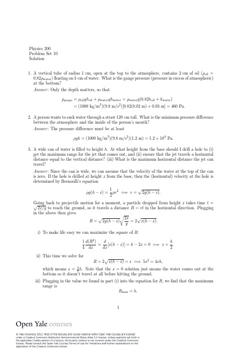
ii) In this case we should not have to integrate at all, and we expect that we can simply apply Bernoulli’s equation at one point to get
R = 2 z(h − z) = z =⇒ 5z2 = 4zh,
which means z
=
4 5
h.
Note that the z
= 0 solution just means the water comes out at the
bottom so it doesn’t travel at all before hitting the ground.
Answer : We can choose the pressure at the equilibrium point to be zero, so that when the cylinder
is a distance z above this point the pressure is −ρgz and hence the force −ρgzA. This causes
Answer : Since the can is wide, we can assume that the velocity of the water at the top of the can is zero. If the hole is drilled at height z from the base, then the (horizontal) velocity at the hole is determined by Bernoulli’s equation
译趣横生

但是某生的答案是: 1)Shit! 2)Hello?
老师在黑板上写了一句:Time is money. 并让同学们翻译。有名学生答道:“汤姆是玛 丽。” 某日刘洪涛遇到外宾,上前搭话曰:I am hongtao liu,外宾曰:我他妈还是方片七呢!
一对热恋中的男女。女生非常没有安全感,于 是对着男友说:“SAY ‘I LOVE YOU!!’SAY IT! SAY IT! SAY IT!” 男的答道:“IT!”
吐槽:外星人真的来过!
英语小笑话
某次英文考试有两道题目: 1)我穿上外套,却发现第一个扣子掉了。 2)他听见电话铃响,就过去接了电话。 正确答案应为: 1)I put on my coat and found its first button was gone. 2)As soon as he heard the phone ringing, he went to pick it up.
谢谢观赏!
一阳指 one finger just like a pen is ( 一只手指像 笔一样?? ) 洗髓经 wash bone (洗骨头?? ) 苗家刀法 maio’’s sword (苗家的刀 ) 易筋经 change your bone (换你的骨头.) 龙象波若功 D and E comble togeter (龙和象的混合 体???) 梯云纵心法 elevator jump (电梯跳跃????) 轻功水上飘 flying skill (飞行技能 ) 小无相功 a unseen power (一种看不见的力量???)
译趣横生
唐雅素
猜一猜
lover
情人
爱人
busboy
餐馆勤杂工
公汽售票员
dead president
大英2第三单元课文翻译

大英2第三单元课文翻译1 If I am thc only parcnt who still corrects his child&apos ;s English, then perhaps my son is right. To him, I am a tedious oddity: a father he is obliged tolis1.en t.o and a man absorberd in the rules af grammar,which my son seems allergic tu.如果我是唯·‘个还在纠正小孩英语的家长,那么我儿了也许是对的。
对他而言,我是‘个乏味的怪物:一个他不得不听其教诲的父亲,一个还沉涎于语法规则的人,对此我儿子似乎期为反感2 l think I got serious about this only recently when I ran into one of my former st.udenls,fresh from an excursion u.a Lurape.“llow was it?" l asked,full ofearncst anticipatisn.我觉得我是在最近偶迥我以前的一位学生时,才开始对这个问题认真起来的。
这个学生刚从欧洲旅游回来。
我满怀若诚挚期待间她:“欧洲之行如何?”3 She nodded three or four times. searched the heavens for the right words, andthen exclaimed,"It was,like,whoa !"她点了三四下头,绞尽脑汁,苦苦寻找恰当的词语,然后惊呼:“真是,咔!”4 And that was it. The civilization of Grocce and the glory of Roman architecture were captured in a condensed non-statement,My student&apas ; : "whoa!" wa8 exc:eedexl only by my hea:l shaking dlistress.没了。
新视野大学英语第三版读写教程第二册Unit3课文及翻译
U3 ACollege life in the Internet age互联网时代的大学生活The college campus, long a place of scholarship and frontiers of new technology, is being transformed into a new age of electronics by a fleet of laptops, smartphones and connectivity 2hours a day.大学校园长久以来都是学术之地,也是新技术的前沿。
现在随着手提电脑和智能手机的大量出现,加上每天2小时不间断的网络连接,大学校园正在转而进入电子设备的新时代。
On a typical modern-day campus, where every building and most outdoor common areas offer wireless Internet access, one student takes her laptop everywhere. In class, she takes notes with it, sometimes instant-messaging or emailing friends if the professor is less than interesting. In her dorm, she instant-messages her roommate sitting just a few feet away. She is tied to her smartphone, which she even uses to text a friend who lives one floor above her, and which supplies music for walks between classes.在典型的现代校园里,每幢建筑和大部分室外公共区域都提供无线互联网接入,学生可以把手提电脑带到任何地方。
全新版大学英语(第二版)综合教程3课文原文及翻译Until1-8较完整版[精品文档]
我们谁也不会忘记第一年的冬天。从12月一直到3月底,我们都被深达5英尺的积雪困着。暴风雪肆虐,一场接着一场,积雪厚厚地覆盖着屋子和谷仓,而室内,我们用自己砍伐的木柴烧火取暖,吃着自家种植的苹果,温馨快乐每一分钟。
7 When spring came, it brought two floods. First the river overflowed, covering much of our land for weeks. Then the growing season began, swamping us under wave after wave of produce. Our freezer filled up with cherries, raspberries, strawberries, asparagus, peas, beans and corn. Then our canned-goods shelves and cupboards began to grow with preserves, tomato juice, grape juice, plums, jams and jellies. Eventually, the basement floor disappeared under piles of potatoes, squash and pumpkins, and the barn began to fill with apples and pears. It was amazing.
Journal of Difference Equations and Applications,
Author QueriesJOB NUMBER:MS256408—JOURNAL:GDEAQ1We have inserted a running head.Please approve or provide an alternative.Q2Please supply received,revised and accepted dates.Q3References[6,10,12]are provided in the list but not cited in the text.Please supply citation details or delete the reference from the reference list.On the Cushing–Henson conjecture,delay difference equations and attenuant cyclesE.BRA VERMAN†{*and S.H.SAKER‡§†Department of Mathematics and Statistics,University of Calgary,2500University Drive N.W,Calgary,Alberta,Canada,T2N 1N4‡Department of Mathematics,Faculty of Science,Mansoura University,Mansoura 35516,Egypt(Received B ;revised B ;in final form B )Q2We consider the second part of the Cushing–Henson conjecture (the cycle’s average is less than the average of carrying capacities;the first part of the conjecture deals with the existence and global stability of periodic cycles)for a periodic delay difference equationx n þ1¼f ðK n ;x n 2h 1ðn Þ;...;x n 2h r ðn ÞÞ:Sufficient conditions on f and h i are obtained,when the second part of the conjecture is valid.We demonstrate,sharpness of these conditions by presenting several counterexamples.In addition,sufficient global attractivity conditions are deduced for the Pielou equation.Keywords :Periodic difference equations;Average population density;Beverton–Holt equation;Pielou equation;Global asymptotic stability AMS Subject Classification :39A11;92D251.IntroductionFor the m -periodic Beverton–Holt equationx n þ1¼l x n1þðl 21Þðx n =K n Þ;l .1;K n .0;ð1:1ÞCushing and Henson [1]proved that,for m ¼2and K 1–K 2the cycle { x 1; x 2}attracts all solutions with x 0.0and satisfies ð x 1þ x 2Þ=2,ðK 1þK 2Þ=2.The Beverton–Holt equation is equivalent to the Pielou equation [3]x n þ1¼a x nn;a .1;b .0;ð1:2Þif we assume a ¼l ,b ¼(a 21)/K ,or K ¼(a 21)/b .However,usually Pielou equation [17,18]is assumed to have a constant delay in the denominator [9].Further,weJournal of Difference Equations and ApplicationsISSN 1023-6198print/ISSN 1563-5120online q 2007Taylor &Francis/journals DOI:10.1080/10236190701565511{Partially supported by the NSERC Research Grant and the AIF Research Grant.§The work was partially implemented at the University of Calgary and supported by the AIF Research Grant.*Corresponding author.Email:maelena@math.ucalgary.caGDEA 256408—24/7/2007——280137Journal of Difference Equations and Applications ,Vol.00,No.0,2007,1–1251015202530354045will refer tox n þ1¼l x n1þðl 21Þðx n 2lK nÞ;l .1;K n .0ð1:3Þas to a delay Beverton–Holt equation (which is equivalent to Pielou equation).Further,Cushing and Henson [2]conjectured that for any p $2(A)there exists a globally asymptotically stable cycle;(B)the average over this stable cycle is less than the average of carrying capacities.Statements (A)and (B)for m -periodic,m $2,Beverton–Holt equation were proved by,Elaydi and Sacker [4,5].The proof of (B)for the Beverton–Holt equation can also be found in Ref.[11]and for a more general equation in Refs.[14,15].Conjectures (A)and (B)are of ecological interest,since they imply that the changing periodic environment leads to eventually less average population density than the average of carrying capacities.Due to ecological importance,it is natural to formulate the following problems:(1)For which difference equationsx n þ1¼f ðK n ;x n ;x n Þ¼g x nK nx n ;x 0$0;n [Z þ¼0;1;2;...;ð1:4Þwith k -periodic carrying capacity {K n },will conjecture (B)hold,once a cycle exists?(2)Suppose the discrete model involves an l -delayx n þ1¼f ðK n ;x n ;x n 2l Þ;x j $0;j ¼2p ;...;21;x 0.0;ð1:5Þwhich adequately describes the fact that,the impact of the changing environment on the birth rate is not immediate.For which f will hypothesis (B)still be valid?In particular,for (1.1)with f ðK n ;x n ;x n 2l Þ¼x n g x n 2l =K n ÀÁwe have,Pielou equation (1.3).(3)For the delay difference equation,with a periodic {K n },x n þ1¼f ðK n ;x n 2h 1ðn Þ;...;x n 2h r ðn ÞÞ;0#h ðn þl Þ¼h ðn Þ;n [Z þ;r [N ;ð1:6Þwhen will (B)hold,if a cycle exists?We recall that m -cycle of the periodic solution x n of the equation (1.4),with p -periodic K j ,is said to be attenuant if its average is less than the average of carrying capacities:1m X m j ¼1 x j ,1k Xk j ¼1K j :ð1:7ÞIn Refs.[14,15],Problem 1was partially solved,in,particular,the following result wasobtained.Lemma 1.1.[14]Let x n be a positive m -cycle of equation (1.4).Suppose that K s –K s þ1for some s [{1,2,...,k },where K s is k -periodic.Assume that xg (x )is strictly concave on an interval (a ,b ),0,a ,b ,containing all points x j /K j [(a ,b ),j ¼1,2,...,mk .Then the cycle {x j }is attenuant.For hypothesis (B),we refer the reader to the solution of Problem 1,we give a partial affirmative answer to Problem 2(a positive cycle is attenuant,under certain additionalGDEA 256408—24/7/2007——280137E.Braverman and S.H.Saker2505560657075808590conditions),and,generally,the negative answer to Problem 3,however,sufficient conditions on f and delays are deduced when (B)is valid for (1.6).An example of the equation (1.3)with variable periodic delays and carrying capacities is presented,where the average of the Q1periodic solution exceeds the average of carrying capacities.In Section 2we generalize the results of [14,15]to the case of delay difference equations with a special kind of periodic delays.In particular,any constant delay satisfies these conditions.In Section 3,we provide sufficient attractivity conditions for the attenuant cycle of delay Beverton–Holt equation (1.3),and illustrate its application by an example.Finally,Section 4outlines some open problems.2.Attenuant cycles of difference equations with variable delaysConsider the difference equation with a periodic reproduction function,which depends on the carrying capacity K n and involves r delaysx n þ1¼f ðK n ;x n 2h 1ðn Þ;...;x n 2h r ðn ÞÞ;x 0[R þ;n [Z þ;r [N ;ð2:1Þwhere R þ¼½0;1Þ,Z þ¼{0;1;...},under the following conditions:(a1)f :R r þ1þ!R þis a continuous function satisfying f ðK n ;K n ;...;K n Þ¼K n ,f ðK n ;x ;...;x Þ.x ,if 0,x ,K n and f ðK n ;x ;;...x Þ,K n ,if x .K n ;(a2){K n }is a k -periodic sequence,K n þk ¼K n and K n .0for all n [Z þ;(a3)h q ðn Þ$0;h q ðn þl Þ¼h q ðn Þ;,n [Z þ;(a4)H q ðn Þ:¼ðn 2h q ðn ÞÞðmod l Þis a one-to-one map of the set {0,1,...,l 21}ontoitself,q ¼1,...,r .Hypothesis (a4)yields that,each H q is a reshuffling of the set {0,1,...,l 21};in other words,this means that each component of f ,beginning with the second one,refers to any element of the sequence x n exactly once.In the following,we will demonstrate that this hypothesis is essential for a cycle to be attenuant.Remark 1.An example of a delay satisfying (a4)is (for some s $0)h ðn Þ¼s ;n is oddh ðn Þ¼s þ2;n is even :For example,in the latter case if s ¼3then n 2h (n )for n ¼1,2,3,4,5,6,7,8,...is 22,23,0,21,2,1,4,3,...,respectively.Here,l ¼2,h (n þ2)¼h (n )and the sequence H (n )¼0.5(12(21)n )is 2-periodic.Remark 2.If (a3)and (a4)hold,then for any multiple of l the hypothesis (a 4)is also valid.Theorem 2.1.Let {p n }be a positive m -cycle of equation (2.1),if such cycle exists.Suppose (a 1)2(a 4)hold,K s –K s þ1for some s [{1,2,...,k },and f (K ,x 1,...,x r )is a strictlyGDEA 256408—24/7/2007——280137Delay difference equations and attenuant cycles395100105110115120125130135concave function in the domain D containing all K s (for the first argument )and all p n (for the others ).Then the cycle {p n }is attenuant.Proof.The strict concavity of f ðK ;x 1;...;x r Þand K s –K s þ1imply the following strict inequality (here functions H q are mod mkl ,see Remark 2)12f ðK s ;p H 1ðs Þ;...;p H r ðs ÞÞþ12f ðK s þ1;p H 1ðs þ1Þ;...;p H r ðs þ1ÞÞ,f 12ðK s þK s þ1Þ;12ðp H 1ðs Þþp H 1ðs þ1ÞÞ;...;12ðp H r ðs Þþp H r ðs þ1ÞÞ :ð2:2ÞBy the assumption of the theorem,f is concave in D .Since,{p n }is an m -periodic solution of (2.1),then p n þ1¼f K n ;p H 1ðn Þ;...;p H r ðn ÞÀÁ.Hence,by (2.2)and the concavity of f ,we have1mkl X mkl n ¼1p n þ1¼1mkl Xmkl n ¼1f ðK n ;p H 1ðn Þ;...;p H r ðn ÞÞ¼1mkl X n ¼1;:::;mkl ;n –s ;s þ1f ðK n ;p H 1ðn Þ;...;p H r ðn ÞÞ"þ212f ðK s ;p H 1ðs Þ;...;p H r ðs ÞÞþ12f ðK s þ1;p H 1ðs þ1Þ;...;p H r ðs þ1ÞÞ !,1mkl X n ¼1;:::;mkl ;n –s ;s þ1f ðK n ;p H 1ðn Þ;...;p H r ðn ÞÞ"þ2f 12ðK s þK s þ1Þ;12ðp H 1ðs Þþp H 1ðs þ1ÞÞ;...;12ðp H r ðs Þþp H r ðs þ1ÞÞ !#f 1mkl X mkl n ¼1K n ;1mkl X mkl n ¼1p H 1ðn Þ;...;1mkl X mkl n ¼1p H r ðn Þ !¼f ð K ; p ;...; p Þ:We recall that,K¼1k X k n ¼1K n ; p ¼1m X m n ¼1p n and note that,the latter equality is due to (a 4).(H i (n )is periodic with period l and {p H i ðn Þ:n ¼1;2;...;mkl }is a reshuffling of the set {p 1;p 2;...;p mkl }).The obtained inequalityp ,f ð K ; p ;...; p Þby (a 1)implies p , K,which completes the proof.ALet us apply Theorem 2.1to the equation with constant delaysx n þ1¼f ðK n ;x n 2s 1;...;x n 2s r Þ:ð2:3ÞCorollary 2.2.Suppose (a 1)and (a 2)hold,s j $0,j ¼1,2,...,r .(1)If k divides s 1;...;s r ,the sequence {K j }is nonconstant and the function of two variablesg ðK ;x Þ¼f ðK ;x ;...;x Þis strictly concave then any k -periodic cycle of (2.3)is attenuant.GDEA 256408—24/7/2007——280137E.Braverman and S.H.Saker4140145150155160165170175180(2)Let {p n }be a positive m -cycle of equation (2.3),the sequence {K j }be nonconstant,andf ðK ;x 1;...;x r Þbe a strictly concave function in the domain D containing all K s (for the first argument )and all p n (for the others ).Then the cycle {p n }is attenuant.Proof.(1)For any k -periodic solution,we havex n þ1¼f ðK n ;x n 2s 1;...;x n 2s r Þ¼f ðK n ;x n ;...;x n Þ¼g ðK n ;x n Þ:Applying Theorem 2.1we deduce that,the cycle is attenuant.(2)follows from Theorem 2.1,since (a3)and (a4)are always valid for constantdelays.ALemma 2.3.Suppose (a 2)and (a 4)hold and K n is a nonconstant sequence.Then any m -cycle of the difference equation (if it exists )x n þ1¼a 0K n þa 1x n 2h 1ðn Þþ...þa r x n 2h r ðn Þ;X r j ¼0a j ¼1;ð2:4Þis attenuant.Proof.Since,the function 1/x is strictly convex and K n is a nonconstant sequence,then1m X m n ¼1p n þ1¼1mkl X mkl n ¼1p n þ1¼1mkl X mkl n ¼1a 0K n þa 1x n 2h 1ðn Þþ...þa rx n 2h r ðn Þ21,1mkl X mkln ¼1ða 0K n þa 1x n 2h 1ðn Þþ...þa r x n 2h r ðn ÞÞ¼a 01k X k n ¼1K n þ1ml X m n ¼1ða 1x n 2h 1ðn Þþ...þa r x n 2h r ðn ÞÞ¼a 01k X k n ¼1K n þð12a 0Þ1m X m n ¼1x n ;which immediately impliesa 01m X m n ¼1x n ,a 01k X k n ¼1K n ;or1m X m n ¼1x n ,1k XKn ¼1K n :This completes the proof.ARemark 3.Strict concavity of the function f in the first argument only,with concavity inother arguments is sufficient,together with (a 1)2(a 4),for a periodic cycle to be attenuant.GDEA 256408—24/7/2007——280137Delay difference equations and attenuant cycles5185190195200205210215220225Remark 4.For r ¼1the equation (2.4)is the delay Beverton–Holt equation [19]x n þ1¼rx h ðn Þ1þðr 21Þx h ðn Þ=K n:ð2:5ÞThus (2.4)generalizes the classic Beverton–Holt equation,such that the Cushing–Henson conjecture on attenuant cycles is still valid.Example 1.Suppose (a2)holds and K n is nonconstant.According to Theorem 2.1and Lemma 2.3,see also [15],any positive cycle of the following equationsx n þ1¼l x n 2l1þðl 21Þðx n 2l =K n Þ;ð2:6Þx n þ1¼ll 2P rj ¼1a j =K n þa 1=x n 2l 1þ...þa r =x n 2l r;a j .0;X r j ¼1a j ,l ;ð2:7Þx n þ1¼exp l 12x n 2lK n&'x n 2l ;l .0ð2:8Þis attenuant.For the above equations,constant delays can be replaced by periodic variable delays satisfying (a4).Besides,if {K n }is an l -periodic sequence,then any l -periodic solution of delay Beverton–Holt equation (1.3)or of the Ricker equationx n þ1¼exp l 12x n 2lK n &'x nis attenuant.The concavity of f ðK ;x 1;...;x r Þis quite expected in the assumptions of Theorem 2.1,since the same requirement is imposed on nondelay equations,as well as (a1)and (a3)are natural restrictions.The new reshuffling condition (a4)means that the system refers to each of the previous conditions exactly once.Example 2demonstrates that if this condition does not hold (some of previous states never appear under f ,while others appear more than once),this can lead to a cycle,which is not attenuant,even if f is strictly concave.Example 2.Consider the delay Beverton–Holt equation with a variable delayx n þ1¼2x n 2h ðn Þ1þðx n 2h ðn Þ=K n Þ;ð2:9Þwhere h (n )¼8j ,if n ¼8j ,8j þ1,...,8j þ5or n ¼8j þ6,and h (n )¼8j þ7,if n ¼8j þ7,j [Z þ.Let K n be 8-periodic:K n ¼1;n ¼8j ;8j þ1;...;8j þ6,and K 8j þ7¼4.Then the solutionp 0¼2;p 1¼41þ2¼43¼p 2¼p 3¼p 4¼p 5¼p 6¼p 7;p 8¼2ð4=3Þ1þð1=3Þ¼2¼p 0is 8-periodic,8 K ¼11;8 p ¼ð34=3Þ.11,thus the 8-cycle is not attenuant.Let us note that,the function f (K ,x )¼2x /(1þx /K )is strictly concave as a function of two variables [15].Example 3demonstrates that if (a4)does not hold for the delay Beverton–Holt equation,this can lead to a stable cycle which is not attenuant.GDEA 256408—24/7/2007——280137E.Braverman and S.H.Saker6230235240245250255260265270Example3.Consider a6-periodic delay Beverton–Holt equation with a variable periodic delayx nþ1¼2x n1þðx tðnÞ=K nÞ;ð2:10Þwhere,tð6nÞ¼tð6nþ1Þ¼tð6nþ2Þ¼tð6nþ3Þ¼tð6nþ4Þ¼6n;tð6nþ5Þ¼6nþ5;ð2:11ÞK6n¼K6nþ1¼K6nþ2¼K6nþ3¼K6nþ4¼1;K6nþ5<0:567573;n¼0;1;2;...ð2:12ÞIf x0¼0.8,then x1<0.888889,x2<0.987654,x3<1.097394,x4<1.219326, x5<1.354807.Here K6nþ5is computed in such a way that,the solution with x0¼0.8is 6-periodic,i.e.K5¼x5x02x52x0¼0:8x52x520:8<0:8Á1:3548072Á1:35480720:8<0:567573:Then x6¼x0¼0:8.Since,x7depends on x5only(any x6nþ1depends on x6n only),then the solution is6-periodic.It is to be noted that,the nondelay autonomous equationy nþ1¼x6ðnþ1Þ¼fðy nÞ¼fðx6nÞ;ð2:13ÞwherefðxÞ¼26xð1þxÞþ25x=K5ð2:14Þis asymptotically stable(seefigure1).Thus the periodic solution,which is 0:8;0:888889;0:987654;1:097394;1:219326;1:354807;0:8;...ð2:15Þis globally asymptotically stable,while its average(<1:058012)exceeds the average of carrying capacities(<0:918284).3.Attractivity conditions for delay Beverton–Holt equationLet us present some sufficient attractivity conditions for the attenuant cycle of the delay Beverton–Holt equationx nþ1¼l x nn2p n;l.1;K n.0:ð3:1ÞTheorem3.1.Suppose K n are p-periodic andlim sup n!1X nþpj¼nl pþ1K j21=K j1þK j21=K j,32þ12ðpþ1Þ;ð3:2ÞGDEA256408—24/7/2007——280137Delay difference equations and attenuant cycles7 275280285290295300305310315then,the positive p -periodic solution x n of (3.1)is a global attractor,i.e.every positive solution x n satisfieslim n !1ðx n 2 x n Þ¼0:ð3:3ÞProof.First,we prove that every positive solution x n ,which does not oscillate about x nsatisfies (3.3).Assume that,x n . x n for n sufficiently large (the proof when x ðn Þ, x n is similar and will be omitted ).Let us make the substitutionx n ¼ x n exp{y n };ð3:4Þy n .0for n sufficiently large.Then (3.3)is equivalent tolim n !1y n ¼0:ð3:5ÞFrom (3.1)and (3.4),we see that y n satisfies the equationy n þ12y n þln 1þB n x n e y n 2p1þB n x n¼0;whereB n ¼l 21K n:ð3:6ÞSince,in (3.6)we have,(1þB n e u )/(1þB n ).1,then y n þ12y n ,0.Thus,y n is a decreasing positive sequence,and therefore there exists a nonnegative limit lim n !1y ðn Þ¼a [½0;1Þ.If a .0,then there exist 1.0and n (1).0,such that for,n $n (1)we have y n 2p .a 21.0,which impliesy n þ12y n ,A n :¼2ln 1þB n x n e a 211þB n x n,0;n $n ð1Þ:ð3:7Þ0.511.5200.51 1.52f(x) in (3.5)x 0.8Figure 1.The reproduction function (2.14)of the difference equation (2.13).We see that,the fixed point 0.8is globally asymptotically stable (the slope is negative and exceeds 21)for all positive initial values,thus the periodic solution (2.15)of (2.10)with parameters (2.11)is globally asymptotically stable.GDEA 256408—24/7/2007——280137E.Braverman and S.H.Saker8320325330335340345350355360Now,since B n and x n are positive periodic functions of period p ,we see that,A n is also a p -periodic negative function and A *#A n #A *,0.Thus (3.7)implies y n þ12y n #A *for n $n 1.The summation of the latter inequality from n (1)to n immediately gives y n #y n ð1ÞþA *½n 2n ð1Þ !21as n !1,which is a contradiction.Hence,a ¼0and therefore y n tends to zero as n !1.Thus (3.3)holds,and any positive solution of (3.1)which does not oscillate about x n tends to the periodic solution.To complete the global attractivity result,we prove that every solution,which is oscillatory about x n ,satisfies (3.3).From the transformation (3.4)it is clear that x n oscillates about x n if and only if y n oscillates about zero.So to complete the proof,we have to demonstrate that (3.5)holds,where y n is a solution of (3.6).DenoteG ðn ;u Þ:¼ln 1þB n x n e u1þB n x n ;then (3.6)takes the formy n þ12y n þG ðn ;y n 2p Þ2G ðn ;0Þ¼0:ð3:8ÞBy the Mean Value theorem,(3.8)can be written asy n þ12y n þF ðn Þy n 2p ¼0;ð3:9ÞwhereF ðn Þ:¼›G ðn ;u Þ›uu ¼z n ¼B n x n e z n1þB n x n e z n ¼B n h n 1þB n h n:Here,h n ¼e z n lies between x n and x n 2p .Let us estimate the upper bound of the positivesolution of (3.1).From (3.1),we see that,x n þ1,l x n ,which implies x n ,l p x n 2p .Substituting this into (3.1),we havex n þ1#l x n 1þðl 21K nÞl 2p x n #l p þ1ðl 21ÞK n :Values of F (n )are increasing in h n ,since (B n u )/(1þB n u )is increasing in u ,so F ðn Þ#B nC n1þB n C n;where C n ¼l p þ1ð21ÞK n 21;B n ¼l 21K n;B n C n ¼l p þ1K n 21K n:If P 1n ¼0F ðn Þ,1,then the sequence y n satisfying (3.9)is also convergent.If y n does not tend to zero,then it is eventually positive (negative )and we arrive to the case of a nonoscillatory solution,which was considered in the beginning of the proof.Thus,it remainsto consider the case P1n ¼0F ðn Þ¼1.Applying the results by Erbe et al.[7],we obtain the attractivity condition for (3.1)in the form (3.2):lim supn !1X n þp k ¼nB kC k 1þB k C k ¼sup n X n þp j ¼n l p þ1K j 21=K j 1þK j 21=K j,32þ12ðp þ1Þ;ð3:10Þwhich completes the proof.AThe following example illustrates Theorem 3.1.GDEA 256408—24/7/2007——280137Delay difference equations and attenuant cycles9365370375380385390395400405Example 4.Let r ¼1.01,K be 2-periodic (p ¼2),K 1¼100,K 2¼101.Then,in (3.10)we choose the largest K j 21/K j for the additional term (the sum of two others is constant due to periodicity)and get 2ð1:01Þ3ð101=100Þ1þð1:01Þ3ð101=100Þþð1:01Þ3ð100=101Þ1þð1:01Þ3ð100=101Þ<21:04062:0406þ1:02012:0201,1:666667<53;where 53¼32þ12ð2þ1Þ,thus,the positive periodic solution of (3.1)is stable.Let us recall [13,16]that the equilibrium r 21of the delay Beverton–Holt equation with constant coefficientsz n þ1¼rz n 1þz n 2p ;r .1;n ¼0;1;2;...ð3:11Þis globally asymptotically stable for p ¼1and is locally asymptotically stable if and only ifr 21r ,2cos p p 2p þ1:ð3:12ÞKocic´and Ladas conjectured ([13],see also [16],p.66)that (3.12)is necessary and sufficient for the global asymptotic stability.Below we demonstrate that for p ¼2and p -periodic coefficients the same conjecture can be proposed.Example 5.Consider the delay Beverton–Holt equation (3.1)with p ¼2.According to the conjecture of Kulenovic´and Ladas the positive equilibrium of (3.12)is globally asymptotically stable if r ,ð122cos ð2p =5ÞÞ21<2:618034:Let us take K 1¼2,K 2¼5.Numerical simulations suggest the same conjecture for the attenuant cycle:the 2-cycle x 1<3:5; x 2<2:4is stable for l ¼2:5,while unstable for l ¼2:8,figure 2.The existence of periodic solutions of (3.1)was considered in [8].Various attractivity results for (3.1)were obtained in [8](for a more general case,where variable coefficients are24681001002003004005002.5 - growth rate 2.8 - growth rateFigure 2.The 2-periodic solution of the delay Beverton–Holt (3.1)difference equation with p ¼2is stable when the growth rate is l ¼2:5and is unstable for l ¼2:8.Here K 1¼2,K 2¼5.GDEA 256408—24/7/2007——280137E.Braverman and S.H.Saker10410415420425430435440445450both in the numerator and the denominator;it is also assumed in Ref.[8]that the delay is a multiple of the period of coefficients;however,this is covered by (3.1),since any multiple of a period is also a period for sequences of coefficients)and in Ref.[12].Let us mention that,unlike [8,12],Theorem 3.1presents explicit attractivity conditions,which have only coefficients involved,not (generally,unknown)periodic solutions.4.Some open problemsFinally,we formulate some open (to the best of our knowledge)problems relevant to theCushing–Henson conjecture on attenuant cycles.(1)Prove or disprove the following conjecture:if the positive equilibrium of (3.11)is locallyasymptotically stable,then the positive p -cycle of (3.1),with l ¼r is globally asymptotically stable.Here we report some simulation results,which indicate that the positive p -cycle of (3.1)seems to be stable even in cases when the relevant (3.11)is unstable.(2)Under which conditions will an attenuant cycle of the delay equation (1.6)be globallyasymptotically stable?(3)We conjecture that if f in (1.6)is convex,then for any positive m -cycle the cycle averageof (1.4)is greater than the average of carrying capacities.We suggest that the proof can follow the scheme of Theorem 2.1.Can we conclude that,the cycle is unstable?AcknowledgementsThe authors are grateful to Profs.S.Elaydi and R.J.Sacker for useful discussions and to the anonymous referee for valuable remarks and comments.References[1]Cushing,J.M.and Henson,S.M.,2001,Global dynamics of some periodically forced,monotone difference equations.Journal of Difference Equations and Applications ,6,859–872.[2]Cushing,J.M.and Henson,S.M.,2002,A periodically forced Beverton–Holt equation.Journal of Difference Equations and Applications ,12,1119–1120.[3]Elaydi,S.,2005,An introduction to difference equations.Undergraduate Text in Mathematics ,3rd edition (New York,USA:Springer).[4]Elaydi,S.and Sacker,R.J.,2005,Nonautonomous Beverton–Holt equations and the Cushing–Henson conjectures.Journal of Difference Equations and Applications ,11(4–5),337–346.[5]Elaydi,S.and Sacker,R.J.,2005,Global stability of periodic orbits of non-autonomous difference equations and population biology.Journal of Differential Equations ,1,258–273.[6]Elaydi,S.and Sacker,R.J.,2006,Periodic difference equations,population biology and the Cushing–Henson conjectures.Mathematical Biosciences ,pp.195–207.Q3[7]Erbe,L.,Xia,H.and Yu,J.S.,1995,Global stability of a linear nonautonomous delay difference equation.Journal of Differential Equations ,151–161.[8]Graef,J.R.,Qian,C.and Spikes,P.W.,1996,Oscillation and global attractivity in a discrete periodic logistic equation.Dynamic System and Applications ,2,165–173.[9]Gyo¨ri,I.and Ladas,G.,1991,Oscillation Theory of Delay Differential Equations (Oxford:Clarendon Press).[10]Gyo¨ri,I.and Pituk,M.,1997,Asymptotic stability in a linear delay difference equation,In Proceedings of SICDEA,Veszprem,Hungary,August 6-11,1995,Gordon and Breach Science,Langhorne,PA.[11]Kocic,V .L.,2005,A note on the nonautonomous Beverton–Holt model.Journal of Difference Equations andApplications ,4–5,415–422.GDEA 256408—24/7/2007——280137Delay difference equations and attenuant cycles 11455460465470475480485490495。
Some Classes of Invertible Matrices in GF(2)
Some Classes of Invertible Matrices in GF(2)James S.Plank∗Adam L.Buchsbaum‡Technical Report UT-CS-07-599Department of Electrical Engineering and Computer ScienceUniversity of TennesseeAugust16,2007The home for this paper is /∼plank/plank/papers/CS-07-599.html.Please visit that link for up-to-date information about the publication status of this and related papers.AbstractInvertible matrices in GF(2)are important for constructing MDS erasure codes.This paper proves that certain classes of matrices in GF(2)are invertible,plus some additional properties about invertible matrices.1IntroductionWe are concerned with the question of whether certain matrices in GF(2)are invertible.This question is important when designing erasure codes for storage applications.If an erasure code is composed solely of exclusive-or operations [1,2,3,4,5,8,9],then it may be represented as a matrix-vector product in GF(2).The act of decoding transforms an original distribution matrix into a square decoding matrix that must be inverted.The process is described for general GF(2w)by Plank[7]and isfirst used in GF(2)by Blomer et al.[2].As such,a fundamental part of defining MDS erasure codes is to construct distribution matrices that result in invertible decoding matrices.This paper does not delve into erasures codes,but instead proves that certain classes of matrices in GF(2)are invertible.It also proves some properties of invertible matrices.2NomenclatureIn GF(2),each element is either0or1;addition is the binary exclusive-or operator(denoted⊕),and multiplication is the binary and operator.When we refer to a matrix M w,that means that M w is a square matrix in GF(2)with w rows and columns.Other information about the matrix is included in the subscripts.We refer to the element in row r and column c of M w as M w[r,c].These are zero-indexed,so the top-left element of M w is M w[0,0],and the bottom-right element of M w is M w[w−1,w−1].We perform arithmetic of row and column indices in M w over the commutative ring Z/w Z.We denote the quantity x modulo w by x w.In particular,because x+w w=x w,we have−1w=w−1w.When context disambiguates,we drop the extra notation;e.g.,−1w=w−1.∗Department of Electrical Engineering and Computer Science,University of Tennessee,Knoxville,TN37996,plank@.‡AT&T Labs-Research,Shannon Laboratory,180Park Avenue,Florham Park,NJ07932,alb@.12.1InvertibilityOne way to test whether a square matrix M is invertible is to perform Gaussian Elimination on it until it is in upper triangular form.Then M is invertible if and only if the result is unit upper triangular.(Basic facts about invertibilityof matrices under simple operations are available in many textbooks,e.g.,Lancaster and Tismenetsky[6].)We define steps of Gaussian Elimination as follows.Let c be the leftmost column with at least two1’s in some M w;let r be the topmost row such that M w[r,c]=1and M w[r,c ]=0for0≤c <c.Then one step of Gaussian Elimination or Elimination Step replaces every row r =r such that M w[r ,c]=1with the sum of rows r and r .An example is in Figure1.Thefirst step of Gaussian Elimination for the matrix in Figure1(a)replaces row2with thesum of rows0and2,and row3with the sum of rows0and3.The resulting matrix is in Figure1(b).(a)(b)(c)Figure1:One step of Gaussian Elimination,and deleting rows and columns that are upper-triangular.When the leftmost columns of a matrix M w have zeros below the main diagonal—i.e.,M[i,j]=0for0≤i< and i<j<w—we say the leftmost columns are in upper triangular form or are upper triangular;if inaddition M w[i,i]=1for0≤i< ,we say the leftmost columns are in unit upper triangular form or are unit upper triangular.Assume the leftmost columns of M w are unit upper triangular,and construct matrix M w ,where w =w− ,by deleting the leftmost columns and top rows of M w.Then M w is invertible iff M w is invertible.For example,since the leftmost two columns of the matrix in Figure1(b)are in unit upper triangular form,we may delete the leftmost two columns and the top two rows to produce the matrix in Figure1(c).This matrix is not invertible; therefore,the matrices in Figures1(a)and1(b)are also not invertible.There are other simple operations that preserve invertibility.Thefirst are what we call row shifting and columnshifting.There are four variants.Each takes an original matrix M w and constructs a new matrix M w∗as follows:•Shifting up by r rows:M w∗[i,j]=M w[i+r w,j],for0≤i,j<w.•Shifting down by r rows:M w∗[i,j]=M w[i−r w,j],for0≤i,j<w.•Shifting left by c columns:M w∗[i,j]=M w[i,j+c w],for0≤i,j<w.•Shifting right by c columns:M w∗[i,j]=M w[i,j−c w],for0≤i,j<w.Obviously,shifting M w up by r rows is equivalent to shifting it down by w−r rows,and shifting M w left by rcolumns is equivalent to shifting it right by w−r columns.Swapping rows and columns preserves invertibility,andsubstituting any row with the sum of it and another row also preserves invertibility.Examples are in Figure2.We denote by I w(rsp.,I w→c)the w×w identity matrix(rsp.,shifted c columns to the right)and by0w the w×w matrix of all zeros.Finally,we say a matrix class M is invertible iff all matrices in M are invertible.3The Matrix Classes D w d,s and S w d,sWe now define two classes of matrices:D w d,s and S w d,s.In both:w>2,0<d<w,and0<s<w.The letters are short for“different”and“same”.We define D w d,s,0to be the base element of D w d,s.We construct D w d,s,0as follows:•Start with D w d,s,0=I w+I w→d.2(a)(b)(c)(d)(e)Figure2:Operations that preserve invertibility.(a)is the original matrix.(b)shifts(a)up by three rows,or down by four rows.(c)shifts(a)left by four rows,or right by three rows.(d)swaps rows3and6.(e)replaces row6with the sum of rows3and6.•Set D w d,s,0[0,w−1]=D w d,s,0[0,w−1]⊕1.•Set D w d,s,0[s,d+s−1w]=D w d,s,0[s,d+s−1w]⊕1.There are w elements of D w d,s,denoted D w d,s,0,...,D w d,s,w−1.D w d,s,i is equal to D w d,s,0shifted i rows down and i columns to the right.Therefore,all elements of D w d,s have the same invertibility.Figure3gives various examples.The intuition is that elements of D w d,s are composed of two diagonals that differ by d columns.There are two extra bits flipped in the matrix,which are s rows apart and adjacent to different diagonals.D73,2,0D73,2,2D73,2,6D71,3,0D71,3,3Figure3:Various examples of matrices in D w d,s.The definition of S w d,s is similar,except the two extra bits that areflipped are adjacent to the same diagonal.As with D w d,s,we define a base element S w d,s,0as follows:•Start with S w d,s,0=I w+I w→d.•Set S w d,s,0[0,w−1]=S w d,s,0[0,w−1]⊕1.•Set S w d,s,0[s,s−1w]=S w d,s,0[s,s−1w]⊕1.As with D w d,s,there are w elements of S w d,s,denoted S w d,s,0,...,S w d,s,w−1.S w d,s,i is equal to S w d,s,0shifted i rows down and i columns to the right.Note that when w is even,there are only w/2distinct elements of S w d,s,because S w d,s,i is .We give examples of S w d,s in Figure4.equal to S wd,s,i+w2w4Simple Relationships on D w d,s and S w d,s that Preserve InvertibilityWe use the following relationships on D w d,s and S w d,s.Lemma1D w d,s is invertible iff D w w−d,w−s is invertible.3S73,2,0S73,2,2S71,3,0S76,3,0S62,3,0=S62,3,3Figure4:Various examples of matrices in S w d,s.D113,4,0D118,7,0Figure5:D118,7,0is constructed from D113,4,0by shifting it four rows up and(4+3)rows to the left.Proof:D w w−d,w−s,0can be derived by shifting D w d,s,0s rows up and s+d columns left.2 Figure5demonstrates Lemma1.Lemma2S w d,s is invertible iff S w d,w−s is invertible.Proof:S w d,s,w−s is identical to S w d,w−s,0.2 Lemma3For s>1,D w d,s is invertible iff S w d,s is invertible.Proof:S w d,s,0can be constructed from D w d,s,0by substituting row s with row s plus row(s−1).2 Figure6demonstrates Lemma3.D113,4,0S113,4,0Figure6:S113,4,0is constructed from D113,4,0by substituting row4with row4plus row3.Lemma4For0<s<w−1,S w d,s is invertible iff S w w−d,s is invertible.Proof:S w w−d,s,0can be constructed from S w d,s,0byfirst substituting row s with row s plus row(s−1)and row0with row0plus row w−1,and then shifting the result d columns to the left.24(a)(b)(c)(d)S113,4,0S118,4,0Figure7:(b)is created by substituting row4with row4plus row3.(c)is created by substituting row0with row0 plus row10.(d)is created by shifting left three columns.Lemma4is demonstrated by Figure7,where each step of converting S113,4,0to S118,4,0is shown.The constraints on s in Lemmas3and4are due to the following.When s=1,adding rows0and1does not have the desired effect of moving row s’s one from one diagonal to the other,because row0has three ones.When s=w−1, adding rows0and w−1has the same problem.For convenience in the sequel,we consider invertibility to be an equivalence relation,so two matrices or matrix classes are equivalent iff they are both invertible or both not invertible.5Our Target Class of Matrices,L,and the Grand Liberation TheoremWe define the class L to be the union of all D w d,s such that:•w>1is odd.•GCD(d,w)=1.•If d is even,s=w−d2.•If d is odd,s=w−d2.Theorem5(The Grand Liberation Theorem)All matrices in L are invertible.The rest of this paper proves the theorem.After demonstrating a few special cases,which include D31,1,the proof proceeds as follows:1.We prove by induction that D w2,w−1is invertible for all odd w.2.For d>2,wefirst show that for any odd d there exists some even d such that D wd,w−d2is equivalent to D wd ,w−d 2.Hence we restrict our attention to even d>2.3.We show that for any even d>2,D wd,w−d2is equivalent to S wd,d2.4.We show that the derived S wd,d2is equivalent to some S wd ,w 2with2<w <w,w even,and GCD(w ,d )=1.5.We show that any S w d,w2with even w>2and GCD(w,d)=1is equivalent to some D w d ,s ∈L such thatw <w.6.A second inductive argument completes the proof,as we can iterate Steps2–5until w =3or d =2in Step5.55.1Step 1:Base Cases for the Global InductionFirst,there are only two D 3d,s ∈L :D 31,1and D 32,2.Their base elements are shown in Figure 8(a)and (b).It is easyto verify that they are invertible.Additionally,Figure 8(c)shows D 52,4,4,which will be used below.It is also easy to verify that it is invertible.(a)(b)(c)(d)(e)D 31,1,0D 32,2,0D 52,4,4D 112,10,10D 112,10,10after two stepsof Gaussian Elimination.Figure 8:Base cases for the inductive proof.We now prove that D w2,w −1is invertible for all odd w .We have already shown in Figure 8that this is truefor w =3and w =5.Let w >5be odd,and assume by induction that D w 2,w −1is invertible for odd 1<w<w .Consider D w 2,w −1,w −1.An example is D 112,10,10,depicted in Figure 8(d).This matrix has a very speci fic format:Allelements of I and I →2are set to one,as are D w 2,w −1,w −1[w −1][w −2]and D w2,w −1,w −1[w −2][w −1].Now,perform two steps of Gaussian Elimination.This will set D w 2,w −1,w −1[w −2,0]and D w2,w −1,w −1[w −1,1]to zero,and D w 2,w −1,w −1[w −2,2]and D w2,w −1,w −1[w −1,3]to one.Figure 8(e)demonstrates for w =11.The resulting matrix’s first two columns are unit upper triangular,so the first two rows and columns may be deleted.Thisyields D w −22,w −3,w −3,which is of the form D w 2,w −1,w −1for some odd 1<w <w .By induction,D w2,w −1,w −1isinvertible.Therefore,D w2,w −1is invertible for all odd w >1.5.2Steps 2–4:Reducing the Problem to S wd,w 2for w Even,GCD (w,d )=1Now consider any D w d,w −d 2∈L such that d is odd.By Lemma 1,this is equivalent to D w w −d,w −w −d 2.Since w −d is an even number,D w w−d,w −w −d 2∈L .Therefore,every element D wd,s ∈L for which d is odd has a corresponding element D w d ,s ∈L for which d is even.Thus we need only prove that the elements D wd,w −d 2∈L with even d are invertible.We proved above that D w 2,w −1is invertible,so we now prove that D wd,w −d 2is invertible for even d >2.Therefore,consider D wd,w −d2such that d >2is even,w >3is odd,and GCD (w,d )=1.Since d >2,it follows that w −w −12=w −12≤w −d 2≤w −2.Since w >3,the smallest value that w −d 2may be is 5−12=2.Therefore,by Lemma 3,D w d,w −d 2is equivalent to S w d,w −d 2,which by Lemma 2is equivalent to S w d,w −(w −d 2)=S wd,d 2.So now consider S w d,d 2,w −d2−1.An example is S 176,3,13,depicted in Figure 9(a).Suppose w >2d .(w will notequal 2d ,because GCD (w,d )=1.)Perform d steps of Gaussian Elimination on S wd,d2,w −d 2−1.This moves the ones in rows w −d through w −1from columns 0through d −1to columns d through 2d −1.In our example of S 176,3,13,six steps of Gaussian Elimination are shown in Figure 9(b).Therefore,when we delete the first d rows and columnsof the resulting matrix,we are left with S w −dd,d2,w −d −d 2−1.Note:w −d is odd;w −d >d ;and since GCD (w,d )=1,GCD (w −d,d )=1.Our example continues in Figure 9(c),where we delete the first six rows and columns ofFigure 9(b)to get S 116,3,7.Iterate this process until it yields S wd,d 2,w −d2−1for d <w <2d .We now perform (w −d )steps of Gaussian Elimination.This moves the leftmost ones in rows (w −d )through (2(w −d )−1)over d columns to the right.Whenwe delete the first w −d rows and columns,we are left with S d d−(w −d ),d 2,d 2−1=S d2d −w,d 2,d 2−1.Since GCD (w,d )=1,GCD (d,2d −w )=1as well.6(a)(b)(c)(d)(e)S 176,3,13Six Elimination StepsS 116,3,7Five Elimination StepsS 61,3,2Figure 9:An example of converting S w d,d 2to S dx,d 2for w =17and d =6.Figure 9(d)shows 11−6=5steps of Gaussian Elimination of S 116,3,7,and Figure 9(e)shows that S 61,3,2results when we delete the first five rows and columns from Figure 9(d).We have thus reduced the original problem to the following:Given S wd ,w2with even w >2and GCD (w ,d )=1,determine whetherS wd ,w2invertible.We address this in the next section.5.3Steps 5–6:Proving that S wd,w 2is Invertible for w Even,GCD (w,d )=1Since w >2,it follows that 1<w 2<w −1.Therefore,by Lemma 4,S w d,w 2is equivalent to S w w −d,w 2,so we may assume that d >w 2.We’re going to break this proof into two cases.The first is when d >w 2+1.Consider S wd,w 2,w2−1.An example of this is S 1611,8,7displayed in Figure 10(a).We perform w −d steps of Gaussian Elimination on S wd,w2,w 2−1.Since d >w 2+1,we know that w −d <w2−1,so the w −d steps of Gaussian Elimination simply move the leftmost ones in rows (w −d )through (2(w −d )−1)over d columns to the right.Deleting the first w −d rows and columnsfrom the matrix,we are left with S d 2d −w,w 2,d −w 2−1.These steps are shown in Figures 10(b)and (c),as S 1611,8,7is converted into into S 116,8,2.(a)(b)(c)S 1611,8,75Elimination StepsS 116,8,2Figure 10:An example of converting S w d,w 2to S d2d −w,w 2for w =16and d =11.As before,since GCD (w,d )=1,we know that GCD (2d −w,d )=1.That w is even implies that 2d −w isalso even.Moreover,since d >w 2+1,we know that 2d −w >1.Therefore,by Lemma 3,S d2d −w,w 2is equivalent to D d 2d −w,w 2.Finally:d −2d −w2=2d −2d +w 2=w 2.7Therefore,D d2d−w,w2=D d2d−w,d−2d−w2,which is an element of L.By induction,D d2d−w,d−2d−w2is invertible,imply-ing that S w d,w2is invertible.The second case is for S w d,w2when d=w2+1and GCD(w,w2+1)=1.An example is S169,8,7shown inFigure11(a).Again,we will perform w−d elimination steps.We will do this in two parts,however.In thefirst part,we perform w−d−1elimination steps.This moves the leftmost ones in rows(w−d)through(2(w−d)−2) over d columns to the right.This is pictured in Figure11(b).The last elimination step replaces two rows of the matrix, because row(w−d)has an extra one adjacent to the diagonal.Therefore,both rows(w−d)and(2(w−d)−1) move their leftmost ones into the column(w−1).This is pictured in Figure11(c).(a)(b)(c)(d)S169,8,76Elimination Steps1More S92,8,0Figure11:An example of converting S w d,w2to S d2,d−1when d=w2+1for w=16.When thefirst w−d rows and columns are deleted from the matrix,we are left with S d2d−w,w2,0.Since d=w2+1,this is equal to S d2,d−1,0(shown as S92,8,0in Figure11(d)).That w>2is even implies that d=w2+1>2isodd,so d−1>1;thus by Lemma3,S d2,d−1is equivalent to D d2,d−1,which we proved invertible in Section5.1. Therefore S w d,w2is invertible.Q.E.D.6The Class O and the Little Liberation TheoremWe now define a third class of matrices,O w d such that w>d≥1.We define O w d,0to be the base element of O w d and construct O w d,0as follows:•Start with O w d=I w+I w→d.•Set O w d,0[0,w−1]=O w d,0[0,w−1]⊕1.Thus,O w d,0is similar to D w d,s,0and S w d,s,0,except it only has one extra one in it,in the top-right corner.There are w elements of O w d,denoted O w d,0,...,O w d,w−1.O w d,i is equal to O w d,0shifted i rows down and i columns to the right. Therefore,all elements of O w d are equivalent.We show some examples of matrices in O w d in Figure12.(a)(b)(c)(d)O73,0O73,6O74,6O21,1Figure12:Examples of matrices in O w d.We start with a simple lemma:8Lemma 6O w d is invertible iff O ww −d is invertible.Proof:O w w −d,w −1can be derived by replacing row w −1of O w d,w −1with the sum of rows w −1and w −2,and shiftingthe resulting matrix d columns to the left.An example is in Figure 12,where O 74,6may be obtained by replacing row 6of O 73,6with the sum of rows 5and 6,and shifting the result three columns to the left.2De fine O to be the union of all O wd such that GCD (w,d )=1.Theorem 7(The Little Liberation Theorem)All matrices in O are invertible.Proof:This proof is far simpler than that of the Grand Liberation Theorem.It,too,is inductive.We start with the base case O 21,an element of which is pictured in Figure 12(d).This matrix is already in unit upper triangular form and is therefore invertible.Now,consider O w d ∈O and suppose by induction that O wd∈O is invertible for all 1≤d <w <w .By Lemma 6and the hypothesis that GCD (w,d )=1,we may assume that d <w 2,or else we consider O ww −d in lieu of O w d .Performing d elimination steps on O w d,w −1moves the leftmost ones in rows w −d through w −1over d columnsto the right.Since d <w 2,these ones will not be moved to the diagonal,nor will the one at O wd,w −1[w −1,w −2]be affected.Therefore deleting the leftmost d columns,which are now unit upper triangular,and top d rows leaves O w −d d,w −d −1.Since GCD (w,d )=1,GCD (w −d,d )=1,and therefore O w −d d,w −d −1∈O .By induction,O w −d dis invertible;therefore O wd is invertible.2An example is depicted in Figure 13where O 125,11is converted to O 75,6by five elimination steps.(a)(b)(c)O 125,11Five elimination stepsO 75,6Figure 13:An example of converting O wd,w −1to O w −d d,w −d −1.7Some Trivial Properties of Matrices in GF (2)The following two lemmas are likely folklore,but we include them for completeness.Lemma 8If some matrix M w has precisely w ones,then M w is invertible iff it is a permutation matrix.Proof:Any permutation matrix is invertible.Conversely,if M w has precisely w ones but is not a permutation matrix,then some row or column contains all zeros,in which case M w is not invertible.2Lemma 9Let M w 1and M w 2be permutation matrices.The sum M w 1+M w2is not invertible.Proof:Let M w =M w 1+M w 2.Suppose there exist r and c such that M w 1[r,c ]=M w2[r,c ]=1.Then row r of M w contains all zeros,so M w is not invertible.Thus,we assume there are no such r and c ;in this case,M has precisely two ones in each row and column.We prove by induction that such matrices are not invertible.The base case is shown in Figure 14(a),which depicts the only M 2with two ones in each row and column.This matrix is clearly not invertible.9Now,let matrix M w for some w>2have exactly two ones in each row and column.Let rows r1and r2be the two rows that have ones in column zero,and let c1,c2>0be such that M w[r1,c1]=M w[r2,c2]=1.Swap row r1with row0,and perform one elimination step.This will set M w[r2,0]=0and M w[r2,c1]=M w[r2,c1]⊕1.If c1=c2, then all of row r2’s elements become zero,so M w is not invertible.If c1=c2,then deleting thefirst row and column leaves a matrix M w−1with exactly two ones in each row and column.By induction,this new matrix in not invertible; therefore M w is also not invertible.2(a)(b)(c)(d)(e)(f)M2.M7,After one elimination M7,After one M6.c1=c2=3.step,Row4is all zeros.c1=3,c2=2.elimination step.Figure14:Matrices with two ones in each row and column.We show examples of the elimination step in Figure14(b)-(f).In Figure14(b),the elimination step,depicted in Figure14(c)turns row4into all zeros.In Figure14(d),the elimination step of the matrix M7results in Figure14(e), which is equivalent to a matrix M6(Figure14(f)).8A Final Theorem on the Invertibility of a Type of(k+2)w×kw MatrixLet row r of some matrix M w contain precisely one one—we call such a row an identity row—and let the one be in column c.By cofactor expansion,deleting row r and column c yields an equivalent matrix M w−1.The remaining theorem concerns a(k+2)×k block matrix A,structured as follows and pictured in Figure15:•Each block is w×w.•Block A[i,i]=I w for0≤i<k.•Blocks A[i,j]=A[j,i]=0w for0≤i<j<k.•Block A[k,j]=I w for0≤j<k.•Block A[k+1,j]=X j for0≤j<k and some given X j.Consider the class A∗of k+22 block matrices induced by deleting any two rows of blocks from A.Theorem10All matrices in A∗are invertible iff(1)every X i is invertible,and(2)for0≤i<j<k,X i+X j is invertible.Proof:Let A∈A∗.There are four cases.Case1:A is composed of thefirst k rows of blocks of A,which form I kw.Case2:A is composed of row k and any k−1of thefirst k rows of blocks of A.Now,A has(k−1)w identity rows.Deleting these rows and their associated columns yields I w.Case3:A is composed of row k+1and any k−1of thefirst k rows of blocks of A;let i be the omitted row of blocks from thefirst k.Again,A has(k−1)w identity rows,which we can delete with their associated columns to yield X i,so A is equivalent to X i.10Figure15:The(k+2)×k block matrix A of w×w matrices over GF(2).Figure16:The2w×2w matrix that results when w(k−2)identity rows are deleted from A in Case4.Case4:A is composed of rows k,k+1,and any k−2of thefirst k rows of blocks of A;let i and j be the omitted rows of blocks from thefirst k.Now A has(k−2)w identity rows,which we can delete with their associated columns to yield the matrix pictured in Figure16.Now,perform w elimination steps on this matrix.For each r and c such that X i[r,c]=1,the elimination step for column c will replace row w+r with the sum of rows w+r and c.This will set X i[r,c]=0and X j[r,c]=X j[r,c]⊕1. After the elimination steps,the leftmost w columns will be upper triangular,and deleting them leaves X i+X j. Therefore,A is equivalent to X i+X j.29AcknowledgementsThis material is based upon work supported by the National Science Foundation under grants CNS-0437508and CNS-0615221.References[1]M.Blaum,J.Brady,J.Bruck,and J.Menon.EVENODD:An efficient scheme for tolerating double disk failuresin RAID architectures.IEEE Transactions on Computing,44(2):192–202,February1995.[2]J.Blomer,M.Kalfane,M.Karpinski,R.Karp,M.Luby,and D.Zuckerman.An XOR-based erasure-resilientcoding scheme.Technical Report TR-95-048,International Computer Science Institute,August1995.[3]P.Corbett,B.English,A.Goel,T.Grcanac,S.Kleiman,J.Leong,and S.Sankar.Row diagonal parity for doubledisk failure correction.In4th Usenix Conference on File and Storage Technologies,San Francisco,CA,March 2004.11[4]J.L.Hafner.WEA VER Codes:Highly fault tolerant erasure codes for storage systems.In F AST-2005:4th UsenixConference on File and Storage Technologies,pages211–224,San Francisco,December2005.[5]J.L.Hafner.HoVer erasure codes for disk arrays.In DSN-2006:The International Conference on DependableSystems and Networks,Philadelphia,June2006.IEEE.[6]ncaster and M.Tismenetsky.The Theory of puter Science and Applied Mathematics.Aca-demic Press,San Diego,CA,second edition,1985.[7]J.S.Plank.A tutorial on Reed-Solomon coding for fault-tolerance in RAID-like systems.Software–Practice&Experience,27(9):995–1012,September1997.[8]J.S.Plank and L.Xu.Optimizing Cauchy Reed-Solomon codes for fault-tolerant network storage applications.InNCA-06:5th IEEE International Symposium on Network Computing Applications,Cambridge,MA,July2006.[9]J.J.Wylie and R.Swaminathan.Determining fault tolerance of XOR-based erasure codes efficiently.In DSN-2007:The International Conference on Dependable Systems and Networks,Edinburgh,Scotland,June2007.IEEE.12。
- 1、下载文档前请自行甄别文档内容的完整性,平台不提供额外的编辑、内容补充、找答案等附加服务。
- 2、"仅部分预览"的文档,不可在线预览部分如存在完整性等问题,可反馈申请退款(可完整预览的文档不适用该条件!)。
- 3、如文档侵犯您的权益,请联系客服反馈,我们会尽快为您处理(人工客服工作时间:9:00-18:30)。
1.The analysis of the main characters
Began with flashback and ‘I’ tone, the film presents us kinds of people, here I divide them into 4 typical groups: 1. Virus, Chauter (the silencer). etc education system ) ( represent the
Virus is arbitrary and test-score-oriented, for the reason of his planning for his son’s fate and which just lead to the death of his son. He is not thoughtful and considerate( the suicide of Raju, for instance) . He’s always ignore the students’ feelings, including his own son’s. Chauter( A typical traditional student, nicknamed ‘the Silencer’) Features: blind-study pride and conceited narrow-minded mean
The analysis of group 2
Rancho ( the central role, a guy be of creativity) Features: creative intelligent brave decisive venturesome helise .etc
The after-thoughts on 3
idiots
The title ‘3 idiots’ made me think of comedy at the first sight. However, after I get to know this film, I was moved. It is a humorous comedy that make you burst out laughing, it is also a tragedy that deepen your conception about every perspective of life. Beyond doubt ,the director did give us a happy ending.
Evidence :Rancho is a representative of a new generation. The first time he showed up, he surprised us with the application of physical knowledge. Leant from the whole film, we found him more creative than we could imagine. Here his creativity not only refers to the achievements he had gained at the last, but also refers to his simple and unique life attitudes that he delivered. Rancho’s motto is ‘ all is well’. He use this simple sentence get through tough things. He is decisive, wise, creative, intelligent when handle with emergencies( to send Ranju’s father to hospital, to asist in Pia’s sister’s child delivery, for instance). He is caring and kind ,he helped his friend out of mental loss, he treated friends as family members. Rancho is venturesome, he dare to challenge conservation. His principle of learning is passion. He is passionate on machine, therefore he loved it and married it. In a word, he is a guy of creative flexibility.
2. Rancho, Joy .etc ( represent the new creative generation) 3. Farhan, Raju .etc (represent the side-walkers that at a loss of fate) 4. Family, Farhan’s parents, Raju’s family burden .etc ( represent the universle conditions that the youth are facing)
The analysis of group 1
Virus ( Director of ICE) Features: competitive traditional conservative stubborn arbitrary test-score-oriented Evidence: virus’ first appearance showed us that he is a competitive man, for he couldn’t bear someone who’s just in front of him( the scene that he rides bike). What’s more ,his speech towards freshmen shaped his feature vividly, that is, his words of ‘ the life begins with murder, that’s the nature, compete or die’ ‘life is a race’( here we can feel the pressure he is delivering to the students). Moreover , his time-saving tie ,shirt and fixed punctual sleep time played important roles in shaping this feature. Virus is traditional, conservative and stubborn on education, he did not advocate new thoughts. What he wanted is to compete fiercely with other universities. The only standard he value a student is score. In his conception of ‘a better score, a better job’, he locate students according to their grades( the scene that the students gathered for a photograph.). Saying Virus is stubborn, I hold this point, that is, considering his authority he just denied his faults( Joy’s death for instance, partly due to his fault. What’s more, Chauter became a victim of conservation due to his fault, still partly.)
Evidence: Chauter is a blind-study student, for he always study without thinking. Take the speech on the opening ceremony day for an example , what he knew is to recite lyrics or something bookish .( the scene of define the machine can also serve as an evidence). Moreover ,in order to develop his memory ability he abused unknown medicine and this contributes to his nickname ‘Silencer’. Chauter is pride and conceited. He enjoys showing off himself, such as his score or his talent( or the later his boasting of his promising career). He is narrow-minded, for he couldn’t new learning approaches, he always remembered to laugh at Rancho and may be some of his classmates. He is mean. He disturbed other students’ review so that it could be easy for him to gain a high mark..( unreasonable way of competing) Frankly saying, Chauter is a tragedy that created by conservation, a victim. ( there exist lots of people as Chauter)