Performance of spatially correlated MIMO channel with antenna selection
外文翻译原文science 2

/locate/rggThe stages and duration of formation of gold mineralizationat copper-skarn deposits (Altai–Sayan folded area )I.V. Gaskov *, A.S. Borisenko, V.V. Babich, E.A. NaumovV.S. Sobolev Institute of Geology and Mineralogy, Siberian Branch of the Russian Academy of Sciences,prosp. Akad. Koptyuga 3, Novosibirsk, 630090, RussiaReceived 20 March 2009; accepted l6 November 2009AbstractGold mineralization at copper-skarn deposits (Tardanskoe, Murzinskoe, Sinyukhinskoe, Choiskoe) in the Altai–Sayan folded area is related to different hydrothermal-metasomatic formations. It was produced at 400–150 ºC in several stages spanning 5–6 Myr, which determined the diversity of its mineral assemblages. Gold mineralization associated with magnetite bodies is spatially correlated with magnesian and calcareous skarns, whereas gold mineralization in crushing zones and along fault sutures in moderate- and low-temperature hydrothermal-metasomatic rocks (propylites, beresites, serpentinites, and argillizites) is of postskarn formation. Different stages were manifested with different intensities at gold deposits. For example, the Sinyukhinskoe deposit abounds in early high-temperature mineral assemblages; the Choiskoe deposit, in low-temperature ones; and the Tardanskoe and Murzinskoe deposits are rich in both early and late gold minerals. Formation of commercial gold mineralization at different copper-skarn deposits is due to the combination of gold mineralization produced at different stages as a result of formation of intricate igneous complexes (Tannu-Ola, Ust’-Belaya, and Yugala) composed of differentiated rocks from gabbros to granites.© 2010, V.S. Sobolev IGM, Siberian Branch of the RAS. Published by Elsevier B.V. All rights reserved.Keywords: gold mineralization; skarns, copper-skarn deposits; hydrothermal-metasomatic formationsIntroductionRecent data on the isotope geology and geochronology of rocks and ores and geological data on the ore genesis gaps proved that ore deposits formed for a much longer time than was assumed earlier (Rundkvist, 1997). This is also true for commercial gold mineralization at many Cu-skarn deposits in the Altai–Sayan folded area (ASFA).Gold-containing Cu-skarn deposits are widespread in many ore districts of the ASFA: Gorny Altai (Sinyukhinskoe,Murzinskoe, Choiskoe), Kuznetsk Alatau (Natal’evskoe, Fe-dorovskoe), Gornaya Shoria (Maisko-Lebedskoe), and Tuva (Tardanskoe, Khopto). Most of them are commercial deposits (Fig. 1).Skarn formation processes at these deposits were related to the Early and Middle Paleozoic granitoid magmatism in the Tannu-Ola (eastern Tuva), Yugala (Sinyukha, northeastern Altai), and Ust’-Belaya (northwestern Altai) intrusive com-plexes (Gusev, 2007; Shokalsky et al., 2000). Formation of commercial gold mineralization was a longer and more intricate process (Gaskov, 2008). In most part of these deposits, gold mineralization is the product of multistage ore process, which is characterized by different mineral composi-tions and spatial occurrences. Almost all these deposits bear gold mineralization spatially and genetically related to skarns and aposkarns in assemblage with magnetite and sulfides (Korobeinikov and Matsyushevskii, 1976; Korobeinikov and Zotov, 2006; Korobeinikov et al., 1987; Vakhrushev, 1972)and gold mineralization isolated from skarns and represented by sulfide-containing (pyrite, chalcopyrite, bornite, chalcocite)hydrothermal products of moderate-temperature assemblage in crushing zones (Shcherbakov, 1974). Often, the deposits also bear epithermal gold-containing assemblage with low-tem-perature sulfides, tellurides, and selenides usually developed at the final stage of mineral formation in rocks of different compositions, including sedimentary, igneous, and skarn (Gas-kov, 2008; Gaskov et al., 2005).The recently obtained ages of ore formation products and igneous rocks (Gaskov, 2008; Rudnev et al., 2004, 2006;Shokalsky et al., 2000) provide a new concept of the sequence of ore formation and its duration and relation with multiphasemagmatism.Russian Geology and Geophysics 51 (2010) 1091–1101*Corresponding author.E-mail address : gaskov@uiggm.nsc.ru (I.V. Gaskov)doi:10.1016/j.rgg.2010.0.0011068-7971/$-see front matter D 2010, IG M, Siberian Branch of the RAS.Published by E lsevier B.V .All rights reserved.V S. .Sabolev 9Let us dwell on the specific features of gold mineralization at particular deposits.Gold mineralization at Cu-skarn depositsThe Tardanskoe deposit is localized in the zone of the Kaa-Khem deep fault, in the exocontact part of the Kopto-Baisyut gabbro-diorite-plagiogranite massif (Fig. 2) (Korobe-inikov and Zotov, 2006; Korobeinikov et al., 1987). At the massif contact, Lower Cambrian volcanogenic-carbonate de-posits are transformed into magnesian and calcareous skarns described in detail earlier (Korobeinikov, 1999; Korobeinikov and Matsyushevskii, 1976; Korobeinikov et al., 1997). The skarn bodies are spatially close to aposkarn metasomatites bearing actinolite, tremolite, epidote, serpentine, chlorite, talc,quartz, carbonate, magnetite, and hematite.Gold mineralization at the deposit is of two types: (1) in skarn-magnetite rocks and (2) in metasomatites of linear crushing zones. These types have specific mineralogical and geochemical features.Gold mineralization in skarn-magnetite ores is widespread at the deposit. It is described elsewhere (Korobeinikov and Matsyushevskii, 1976; Korobeinikov and Zotov, 2006; Koro-beinikov et al., 1987; Kudryavtseva, 1969). Gold is spatially related to areas of sulfide mineralization, and its contents are in direct correlation with the amount of sulfide minerals.Gold-sulfide mineralization is extremely unevenly distributed and is localized at the sites of magnetite ores that underwent cataclasis as well as in magnetite microcracks and interstices.The total amount of sulfides (pyrite, chalcopyrite, bornite, and scarcer sphalerite, pyrrhotite, and arsenopyrite) is 1–3%. Gold occurs as fine thin (0.3–0.01 mm) native segregations. This is mainly high-fineness gold (820–990) (Fig. 3, a ) with impuri-ties of silver (up to 13.6%) and copper (up to 5.07%).According to Korobeinikov (1999) and Korobeinikov and Matsyushevskii (1976), the temperatures of formation of magnetite ores were 430–550 ºC, whereas the gold-sulfide assemblage and the hosting metasomatites (actinolite, tre-molite, serpentine, talc) were produced at 250–320 ºC (Gaskov et al., 2005; Vakhrushev, 1972).Gold mineralization in crushing zones is localized in steeply dipping linear tectonic structures of NW, NE, and NS strikes (Fig. 2), which develop after different rocks, including volcanosedimentary, igneous, and skarn ones. These zones reach several hundred meters in length and few tens of meters in width. The petrographic composition of these zones is di-verse and depends mainly on the composition of initial rocks that underwent transformation later. The rocks are metaso-matic, close in composition to propylites, listwaenites, talc-containing and sericite-quartz metasomatites, and beresite-like rocks. Almost each type of hydrothermal-metasomatic rocks is intimately associated with ore minerals. Though the total volume of these minerals does not exceed 3–5%, they are extremely diverse in composition and are extremely unevenly distributed. Along with sulfide minerals typical of Cu-skarn deposits (chalcopyrite, pyrite, bornite, chalcocite,digenite, sphalerite, galena), the mineralized zones of the deposit abound in tellurides—hessite (Ag 2Te), tellurobis-muthite (Bi 2Te 3), and tetradymite (Bi 2Te 2S),—and low-tem-perature Co and Ni sulfides and sulfoarsenides (Table 1). The latter have a variable composition and often consist of intermediate phases of continuous mineral series, e.g., allo-clasite(CoAsS)–arsenopyrite(FeAsS) or siegenite(CoNi 2S 4)–violarite(FeNi 2S 4).Gold occurs mainly as native fine thin (0.01–0.5 mm)disseminations in rock microcracks and as inclusions in pyrite,chalcopyrite, and bornite. The gold fineness varies over a broad range of values—from 440 to 820 (Fig. 3, b ). The lowest-fineness gold segregations are compositionally similar to electrum and have high contents of Ag (up to 54.78%) and Hg impurity (up to 3.65%).On the flanks of mineralized crushing zones, there is sometimes gold mineralization in low-temperature argillitized rocks of chlorite-kaolinite-carbonate-hydromica composition.This gold is of low fineness (no more than 600). The mainimpurities are Ag (20–66%) and Hg (up to 5.47%). The formation temperatures of sulfide-telluride assemblages andFig. 1. Schematic occurrence of gold-bearing Cu-skarn deposits in the Altai-Sayan folded area: 1, Murzinskoe; 2, Sinyukhinskoe; 3, Choiskoe; 4, Maisko-Lebedskoe;5, Fedorovskoe; 6, Natal’evskoe; 7, Tardanskoe; 8, Kopto.1092I.V. Gaskov et al. / Russian Geology and Geophysics 51 (2010) 1091–1101gold mineralization in metasomatites and argillitized rocks are within 200–75 ºC.The Murzinskoe deposit is localized at the contact of a small stock-like granodiorite body of the Ust’-Belaya gabbro-diorite complex (Fig. 4). In the exocontact zone, calcareous skarns composed of garnet, pyroxene, wollastonite, and mag-netite develop after the calcareous sandstones of the Murzinka Formation (D1-2). In the local zones, there are aposkarnFig. 2. Schematic geologic structure of the Tardanskoe deposit (compiled after the data of K.M. Kil’chichakov and L.V. Kopylova and our new data). 1–4, Lower Paleozoic deposits: 1, andesitic porphyrites and tuffs with siltstone and sandstone interbeds in the lower part of the Tumat-Taiga Formation (Cm 1tm 1); 2, quartz porphyrites with interbeds of andesitic porphyrites and limestones in the upper part of the Tumat-Taiga Formation (Cm 1tm 2); 3, limestones and calcareous shales of the Tapsa Formation (Cm 1tp); 4, Lower and Middle Silurian conglomerates and sandstones (S 1-2); 5, Quaternary deposits (Q IV ); 6, 7, Lower Paleozoic igneous rocks of the Tannu-Ola complex (γδO 1-2): 6, gabbro-diorite-plagiogranite formation; 7, small granite-porphyry and quartz diorite bodies; 8, calcareous and magnesian skarns; 9, hydrothermal-metasomatic rocks in mineralized crushing zones; 10, gold orebodies; 11, tectonic zones; 12, geologic boundaries.I.V. Gaskov et al. / Russian Geology and Geophysics 51 (2010) 1091–11011093Fig. 3. Variations in gold fineness in gold ores from skarn-magnetite bodies (a) and in ores from mineralized crushing zones (b) at the Tardanskoe deposit.Table 1. Mineral parageneses in gold-bearing ores produced at different stages and composition of host rocks at Au-Cu-skarn depositsDeposit Early aposkarn Au-sulfide mineralization in magnetite-skarn rocks Late Au-telluride-sulfide mineralization in superposed crushingzonesOre parageneses Host rocks Ore parageneses Host rocksTardanskoe Magneite (Fe3O4)Pyrite (FeS2)Chalcopyrite (CuFeS2)Bornite (Cu5FeS4)Sphalerite (ZnS)Pyrrhotite (FeS)Arsenopyrite (FeAsS)Gold (Au)Magnesian skarns (pyroxene +fassayite + phlogopite +pargasite + forsterite + spinel).Calcareous skarns (pyroxene +garnet + epidote +wollastonite + skapolite).Aposkarn serpentine andserpentine-chlorite rocksCobaltite (CoFe)AsSGlaucodot (Co,Fe)AsSSiegenite (CoNi2S4)Violarite (FeNi2S4)Hessite (Ag2Te)Gold (Au)Propylites, listvaenites, talc-serpentine-containing andsericite-quartz metasomatites,and argillitized rocksMurzinskoe Magnetite (Fe3O4)Chalcopyrite (CuFeS2)Pyrite (FeS2)Bornite (Cu5FeS4)Sphalerite (ZnS)Galena (PbS)FahloreArsenopyrite (FeAsS)Clinobisvanite (BiVO4)Gold (Au)Calcareous skarns (garnet +pyroxene + wollastonite).Aposkarn metasomatic rocks(quartz + epidote + chlorite +actinolite)Cinnabar (HgS)Metacinnabarite (HgS)Bismuthine (Bi2S3)Aikinite (CuPbBiS3)Emplectite (CuBiS2)Berryite [Pb2(Cu,Ag)3Bi5S11]Naumannite (Ag2Se)Polybasite (Ag16Sb2S11)Barite (BaSO4)Gold (Au)Quartz and quartz-carbonateveins, near-vein metasomatitesof quartz-chlorite-carbonatecomposition, and argillitizedrocksSinyukhinskoe Magnetite (Fe3O4)Pyrite (FeS2)Chalcopyrite (CuFeS2)Bornite (Cu5FeS4)Chalcocite (Cu2S)Sphalerite (ZnS)Pyrrhotite (FeS)Cubanite (CuFe2S3)Gold (Au)Wollastonite, garnet-wollastonite, garnet-pyroxeneand pyroxene skarns, andaposkarn metasomatic rocks(chlorite + actinolite + calcite)Tetradymite (Bi2TeS)Siegenite (CoNi2S4)Cobaltite ((CoNiFe)AsS)Melonite (NiTe2)Wittichenite (Cu3BiS3)Hessite (Ag2Te)Petzite (AuAg3Te2)Altaite (PbTe)Clausthalite (PbSe)Gold (Au)Local zones of actinolite-chlorite-calcite-quartzcompositionChoiskoe Magnetite (Fe3O4)Pyrite (FeS2)Chalcopyrite (CuFeS2)Gold (Au)Garnet, garnet-pyroxene,garnet-wollastonite, andpyroxene-epidote skarnsTetradymite (BiTe2S)Ingodite (Bi2TeS)Joseite (Bi4TeS2)Hedleyite (Bi2Te)Tellurobismuthite (Bi2Te3)Bismuthite (Bi2S3),Native bismuth (Bi)Gold (Au)Quartz and quartz-carbonateveins and quartz-carbonate-chlorite metasomatites1094I.V. Gaskov et al. / Russian Geology and Geophysics 51 (2010) 1091–1101metasomatic rocks consisting of quartz, epidote, calcite,chlorite, actinolite, and, more seldom, tourmaline, apatite, and rodonite.Gold mineralization at the Murzinskoe deposit was earlier ascribed to gold-skarn type. But recent data have shown that only a minor part of the deposit ores — scarce postskarn sulfide mineralization spatially associated with skarn-magnet-ite bodies—can be referred to this type. Most of the commer-cial ores occur in mineralized crushing zones. They form gold-sulfide mineralization in quartz and quartz-carbonate veins and near-vein metasomatites in a 300–400 m thick zone stretching in the N-NW direction for more than 3 km (Fig. 4).The crust of weathering widespread at the deposit contains hypergene copper minerals: malachite, chrysocolla, azurite,chalcocite, coveline, and high-fineness gold.Gold-sulfide mineralization spatially associated with skarn-magnetite bodies is superposed on skarn rocks. It was produced either at the regressive stage of the skarn formation or at the postskarn hydrothermal-metasomatic stage and was accompanied by the formation of moderate- and low-tempera-ture metasomatic minerals—chlorite, actinolite, epidote, and quartz. Sulfide mineralization is unevenly distributed and occurs as veinlet-disseminated chalcopyrite, pyrite, bornite,and sphalerite. It amounts to few percent. Gold occurs as fine thin (0.5–0.01 mm) native segregations. It is mainly of high fineness (840–994) (Fig. 5, a ).In crushing zones (Fig. 4), gold mineralization was found in quartz-carbonate-sulfide veinlets and veins in hydrothermal-metasomatic rocks of quartz-chlorite-carbonate composition with kaolinite, hydromica, and adularia (argillizite formation)developing after different rocks—skarns, hornfelses, shales,siltstones, and limestones,—often beyond skarning and horn-felsing zones. The quartz veins are 0.1 to 2.0 m (on average,0.4 m) thick, of N-S strike and eastern dip. In contrast to the gold-skarn-magnetite type, this mineralization is of more complex composition. In addition to minerals typical of skarn deposits (chalcopyrite, pyrite, bornite, sphalerite, and galena),it includes fahlore, arsenopyrite (FeAsS), cinnabar (HgS),metacinnabarite (HgS), bismuthine (Bi 2S 3), aikinite (CuPb BiS 3), emplectite (CuBiS 2), berryite [Pb 2(Cu,Ag)3Bi 5S 11],naumannite (Ag 2Se), polybasite (Ag 16Sb 2S 11), scheelite (Ca 3WO 4), hematite (Fe 2O 3), clinobisvanite (BiVO 4), bariteFig. 4. Schematic geologic structure of the Murzinskoe deposit. 1, mica-sili-ceous shales (O 1); 2, sandstones, siltstones, and aleuropelites (S 1); 3, terri-genous-carbonate deposits (D 1-2): a , conglomerates, b , limestones, c , sand-stones; 4, granodiorites of the Ust’-Belaya complex (D 3); 5, altered rocks and metasomatites: a , hornfelses, b , skarns, c , quartz-tourmaline metasomatites;6, mineralized crushing zones; 7, faults: a , established, b , predicted; 8, other types of mineralization: a , Murzinka-3 (Au), b, skarn Fe.Fig. 5. Variations in the fineness of gold associated with skarn-magnetite bodies (a ) and gold from ores of mineralized crushing zones (b ) at the Murzin-skoe deposit.I.V. Gaskov et al. / Russian Geology and Geophysics 51 (2010) 1091–11011095(BaSO 4), and gold (Table 1). The content of gold in the ores varies over a broad range of values, from 0.1 to 232 ppm.This gold occurs as fine (<0.1 mm) thin segregations in assemblage with sulfides. Its fineness also greatly varies (640–840), but, compared with the first type of ores, low-fine-ness gold prevails here (Fig. 5, b ).The presence of cinnabar, sulfides and sulfosalts of Bi, Se,and Sb, and barite, predominance of low-fineness gold and electrum, and low-temperature wallrock alteration (formation of kaolinite, hydromica, and adularia) differ these ores from earlier formed ores in skarn-magnetite bodies. The gap between the skarn and ore formation processes is evidenced from the presence of basite dikes cutting the skarns, which bear superposed gold mineralization of this type. At the same time, the presence of gold–cinnabar intergrowths and fine dissemination of gold in cinnabar, presence of Hg-minerals (cinnabar, Hg-sphalerite, saucovite) in the ores, and high contents of As, Sb, and Ti (typical elements of many Au-Hg deposits) permit this mineralization to be referred to as epithermal Au-Hg type (Borisenko et al., 2006). Thermometric studies showed that the homogenization temperatures of fluid inclusions in quartz veins in the northern and central parts ofthe mineralized zone are 215–200 ºC and decrease to 160–130 ºC in the southern part.Fig. 6. Schematic geologic structure of the Sinyukhinskoe deposit (compiled by Gusev (2007) and supplemented by our data). 1, loose Quaternary deposits; 2–6, rocksof the Choya (O 1cs), Elanda (C−2-3el), Ust’-Sema (C −2us), and Upper Ynyrga (C −2vy) Formations: 2, conglomerates, 3, siltstones, 4, sandstones, 5, limestones,6, andesite-basaltic porphyrites; 7–9, rocks of the Yugala (Sinyukha) complex: 7, granites and granodiorites of the early phase (γδD 2-3), 8, granites of the late phase (γD 2-3), 9, dolerite and gabbro-dolerite dikes; 10, plagiogranites of the Sarakoksha complex (ν C −2); 11, skarns; 12, sites with gold mineralization (1, Pervyi Rudnyi (First Ore), 2, Zapadnyi (Western), 3, Faifanov, 4, West Faifanov, 5, Ynyrga, 6, Nizhnii (Lower), 7, Tushkenek, 9, Gorbunov); 13, faults.1096I.V. Gaskov et al. / Russian Geology and Geophysics 51 (2010) 1091–1101The Sinyukhinskoe deposit is localized in northeastern Altai, at the contact of the large (600 km 2) complex Sarakok-sha pluton and Cambrian volcanosedimentary strata of the Ust’-Sema Formation (Shcherbakov, 1967; Vakhrushev, 1972)(Fig. 6). According to Shokalsky et al. (2000) and Gusev (2007), this massif includes the Lower Cambrian Sarakoksha diorite-tonalite-plagiogranite complex and Lower Devonian Yugala gabbro-diorite-granite complex (Sinyukha complex (Gusev, 2003)). It is in the latter complex that the commercial mineralization of the Sinyukha ore field is localized. In the contact zone of the Sinyukha massif, skarns of different compositions are developed in horizons of carbonate rocks and tuffs. Wollastonite and garnet-wollastonite varieties are the most widespread, and garnet-pyroxene and pyroxene ones are scarcer. Near the contact with basic effusive bodies, small magnetite orebodies have been revealed among garnet-py-roxene skarns.Gold mineralization occurs mainly among wollastonite,garnet-wollastonite, and pyroxene-wollastonite skarns and is intimately associated with an assemblage of sulfide minerals.The latter are dominated by bornite, chalcocite, chalcopyrite,and pyrite, which compose ore zones in these rocks and are present in the form of nest-disseminations and stockworks. In local zones of actinolite-chlorite-calcite-quartz composition we found minor amounts of sphalerite, pyrrhotite, cubanite, and tetradymite. There are also occasional findings of rare miner-als, such as siegenite (CoNi 2S 4), cobaltite ((CoNiFe)AsS),melonite (NiTe 2), wittichenite (Cu 3BiS 3), gessite (Ag 2Te),petzite (AuAg 3Te 2), altaite (PbTe), and clausthalite (PbSe)(Table 1). The total content of sulfides does not exceed 5–10%. The sulfides are extremely unevenly distributed—from occasional dissemination to densely disseminated, almost massive ores. The composition of sulfide mineralization slightly changes with depth: Gold-chalcocite-bornite assem-blage is changed by gold-chalcopyrite one. The accumulation of gold-sulfide mineralization was accompanied by the hy-drothermal-metasomatic alteration of the host skarns with the formation of actinolite, chlorite, and calcite near ore veins and nests. Magnetite ores are poorer in gold, and sulfide-free rocks(marbles and diorite-porphyry and granite-porphyry dikes)virtually lack it.Fig. 7. Variations in gold fineness in ores from the Sinyukhinskoe deposit.Fig. 8. Schematic geologic structure of the Choiskoe deposit (compiled by Gusev and Gusev (1998) and supplemented by our data). 1–5, rocks of the Ishpa (O 1is) andTandosha (C−2-3td) Formations: 1, conglomerates, 2, siltstones, 3, sandstones, 4, limestones, 5, felsic tuffs; 6–7, granitoids of the Yugala complex: 6, granites and granodiorites of the early phase (γδD 2-3), 7, leucocratic granites of the late phase (γD 2-3); 8, granite-porphyry, diorite, and lamprophyre dikes (γδD 2-3); 9, skarns;10, gold mineralization occurrences (1, occurrence of the Central skarn deposit, 2, Pikhtovyi, 3, Smorodinovyi); 11, faults.I.V. Gaskov et al. / Russian Geology and Geophysics 51 (2010) 1091–11011097Gold often occurs in ores as native segregations in the form of hooks, fine wires, lumps, and sheets intimately intergrown with bornite, chalcocite, and chalcopyrite. Sometimes, native gold segregations are observed as fine inclusions in cracks and interstices of skarn minerals, most often, wollastonite. These gold particles are mainly no larger than hundredths of millimeter. The gold of primary ores of the Sinyukhinskoe deposit is of high fineness varying over a narrow range of values (911–964) (Fig. 7). The fineness of gold decreases to 860–870 only in its parageneses with tellurides, selenides, and rare sulfide minerals (Roslyakova et al., 1999). The main impurities in gold are silver (up to 19%) and copper (up to 1.7%). The content of Hg does not exceed 0.1%. By the formation conditions, these ores are postskarn hydrothermal,with their deposition temperatures not exceeding 350 ºC (Roslyakova et al., 1999; Shcherbakov, 1972).The Choiskoe deposit is localized 20 km northeast of the Sinyukha ore field, in the zone of contact between the Upper Cambrian terrigenous-carbonate deposits of the Ishpa Forma-tion and the Choya granitoid massif referred to the Lower Devonian Yugala gabbro-diorite-granite complex (Fig. 8). The Choya granitoid massif is small at the surface (1 × 5 km) and extends from west to east, tracing the Choya fault (Gusev,2007). The deposit abounds in dikes of dolerite porphyrites,diorites, and granite-porphyry and in rocks of the lamprophyre series—kersantites, minette, and spessartites. The zone of contact between the granitoids of the Choya massif and the horizons of limestones and terrigenous-carbonate rocks is composed of skarns, which form linear zones extending in the NE direction, like the other rocks. Most bodies are of persistent thickness, ~100 m. By composition, the skarn bodies are divided into zones of garnet, garnet-pyroxene, pyroxene,garnet-wollastonite, and pyroxene-epidote skarns. In the skarn zones and near lamprophyre bodies, poor scheelite-molybde-nite mineralization in quartz veins was established (Gusev,1998).Gold mineralization at the deposit occurs in linear tectonic zones and is not spatially associated with skarns. It develops as quartz veins and quartz-carbonate and quartz-carbonate-chlorite veinlets and nests with gold-sulfide mineralization in crushing and brecciation zones in both the skarns and the granitoids of the Choya massif (Fig. 8).The mineral composition of these objects is nearly the same—gold-sulfide and gold-telluride parageneses. A numberof rare tellurides have been revealed among the Choya deposit ores: tetradymite (BiTe 2S), ingodite (Bi 2TeS), joseite (Bi 4TeS 2), hedleyite (Bi 2Te), tellurobismuthite (Bi 2Te 3), bis-muthine (Bi 2S 3), and native bismuth (Table 1). Magnetite,pyrite, and chalcopyrite, typical minerals of Cu-skarn deposits,are extremely scarce here. The total content of sulfides does not exceed few percent. They occur mainly as fine thin dissemination and do not form large accumulations and nests.Gold in the Choya deposit ores occurs as fine inclusions in sulfide and telluride minerals in quartz veinlets and as intergrowths with ore minerals. The gold particles are hun-dredths and tenths of millimeter in size. By chemical compo-sition, the gold is divided into two groups: medium-fineness (843–880) and high-fineness (940–959); the latter is probably of exogenous nature (Fig. 9). The gold contains Ag (3–12.5 wt.%) and Hg (0–0.48 wt.%) impurities and Cu traces.The thermometric studies showed that homogenization of primary gas-liquid inclusions into liquid proceeds at 126–150 ºC in quartz and at 105–128 ºC in calcite from ore-bear-ing veins.The sequence and duration of formation of gold mineralization and its correlation with magmatism As seen from the above data, gold mineralization at all considered Cu-skarn deposits has a complex multistage for-mation history. But the same stages at different deposits ran with different intensities. For example, at the Sinyukhinskoe deposit, mainly early high-temperature mineral assemblages are widespread, whereas at the Choiskoe deposit, low-tempera-ture ones. The Tardanskoe and Murzinskoe deposits bear both early and late minerals. To elucidate the peculiarities of gold-ore formation, establish the correlation between different types of gold mineralization and magmatic activity, and evaluate the duration of ore formation, we performed Ar-Ar and U-Pb dating of different mineralization and igneous rocks from the Tardanskoe and Murzinskoe deposits.Our investigations have shown that the formation of gold mineralization at the Tardanskoe deposit lasted for a longer time than it was supposed earlier. Skarn mineralization formed at the contact of diorites with carbonate rocks as a result of the intrusion of the Kopto-Baisyut massif. Ar-Ar biotite dating of the massif yielded an age of 485.7 ± 4.4 Ma corresponding to the Early Ordovician (Table 2). The skarns at the massif contact as well as magnetite ores and gold-sulfide mineraliza-tion (pyrite, chalcopyrite, pyrrhotite, bornite, gold) spatially and genetically associated with skarn-magnetite bodies are of similar age. Gold was deposited together with sulfides, as evidenced from the direct correlation between the contents of gold and sulfides (especially chalcopyrite) and from gold inclusions in the sulfides. The formation of skarn and aposkarn mineralization was followed (with some temporal gap) by the intrusion of dike and stock-like small granitoid bodies, which is indicated by their cutting of the sulfide-bearing skarn and magnetite bodies. Ar-Ar dating of these granite bodies yielded an age of 484.2 ±4.3 Ma (Table 2).Fig. 9. Variations in gold fineness in ores from the Choiskoe deposit.1098I.V. Gaskov et al. / Russian Geology and Geophysics 51 (2010) 1091–1101。
Channel Estimation for LTE

ii
Contents
1 Introduction 2 LTE Downlink: Physical Layer
2.1 Overview . . . . . . . . . . . . . . . . . . . . . . . . . . . . . . 2.2 Structure of Pilot Symbols . . . . . . . . . . . . . . . . . . . . 2.3 System Model . . . . . . . . . . . . . . . . . . . . . . . . . . . 3.1 Least Squares Channel Estimation . . . . . . . . . . . . 3.2 Linear Minimum Mean Square Error Channel Estimation 3.2.1 LMMSE Channel Estimation for Spatially Uncorrelated Channels . . . . . . . . . . 3.2.2 LMMSE Channel Estimation for Spatially Correlated Channels . . . . . . . . . . . 3.3 Approximate LMMSE Channel Estimation . . . . . . . . 3.4 Simulation Results . . . . . . . . . . . . . . . . . . . . . 3.4.1 Comparison of Interpolation Techniques . . . . . 3.4.2 LMMSE Channel Estimation . . . . . . . . . . . 3.4.3 ALMMSE Channel Estimation . . . . . . . . . . 4.1 4.2 4.3 4.4 Least Square Channel Estimation . . . . . . . . . . . . . Linear Minimum Mean Square Error Channel Estimation Approximate LMMSE Channel Estimation . . . . . . . . Simulation Results . . . . . . . . . . . . . . . . . . . . . 4.4.1 Comparison of Fast Fading Channel Estimation . 4.4.2 Block Fading Channel Estimation . . . . . . . . . 4.4.3 ALMMSE Channel Estimation . . . . . . . . . .
【豆丁推荐】-相关阴影Rician信道上广义矩形MQAM的性能

相关阴影R ician 信道上广义矩形MQA M 的性能江林超, 李光球(杭州电子科技大学通信工程学院,杭州310018) 摘要:本文使用矩生成函数方法推导了相关视距(LOS )分量和独立散射分量条件下的多输入多输出阴影R ician 衰落信道上采用正交空时分组编码(OST BC )的广义矩形M 进制正交幅度调制(MQAM )的平均误符号率(SEP )的精确闭合表达式。
利用该表达式可计算信道衰落参数以及天线间的相关性对广义矩形MQAM 平均SEP 性能的影响。
数值计算结果阐明,天线间的相关性恶化了广义矩形MQAM 的平均SEP 性能,广义矩形MQAM 的平均SEP 性能随着信道衰落参数的增大而得到改善。
关键词:误符号率;阴影R ician 衰落;多输入多输出系统;正交空时分组码 中图分类号:T N911 文献标识码:A 文章编号:100328329(2009)0320010204Perf or mance of General Rectangular QA M over CorrelatedShado wed Rician Fading ChannelsJ I A NG L in 2chao, L I Guang 2qiu(School of Communicati on Engineering,Hangzhou D ianzi University,Hangzhou 310018,China )Abstract:U sing the moment generating functi on -based analysis app r oach,we derive the exact cl osed -fr o m average sy mbol err or p r obability (SEP )ex p ressi on of orthogonal s pace -ti m e bl ock codes (OST BCs )with general rectangularM -ary quadrature a mp litude modulati on (MQAM )over shadowed R ician multi p le -input multi p le -out put (M I M O )fading channel where the line -of -sight (LOS )component is correlated and the scattered component is s patially white .The above ex 2p ressi ons can be used t o investigate the i m pact of fading para meters and the correlati on bet w een the antennas on the average SEP of general rectangular MQAM.Numerical results show that the SEP perf or mance of general rectangularMQAM deteri orates with increased correlati on bet w een the anten 2nas,and i m p r oves with increased channel fading para meters .Key words:sy mbol err or p r obability (SEP );shadowed R ician fading;multi p le -input multi p le -out put (M I M O )syste m s;orthogonal s pace -ti m e bl ock codes (OST BCs )—01—《无线通信技术》2009年第3期3基金项目:国家自然科学基金项目(60772067);浙江省教育厅科技计划重点项目(20060268)。
相关阴影Rician衰落信道上MPSK的性能
相关阴影Rician衰落信道上MPSK的性能江林超;李光球【摘要】研究多输入多输出相关阴影Rician衰落信道上正交空时分组编码M进制相移键控的平均符号错误概率性能.当信道衰落参数为正整数时,使用矩生成函数方法推导了相关视距分量、独立散射分量条件下的阴影Rician衰落信道上M进制相移键控平均符号错误概率性能的精确闭合表达式.利用获得的精确闭合表达式可以分析信道衰落参数和天线间的相关性对M进制相移键控平均符号错误概率性能的影响.【期刊名称】《杭州电子科技大学学报》【年(卷),期】2010(030)001【总页数】4页(P14-17)【关键词】多输入多输出系统;阴影莱斯衰落;相移键控;空时分组编码;错误概率【作者】江林超;李光球【作者单位】杭州电子科技大学通信工程学院,浙江,杭州,310018;杭州电子科技大学通信工程学院,浙江,杭州,310018【正文语种】中文【中图分类】TN9110 引言衰落信道上空时分组码(Space-Time Block Code,STBC)的性能研究是当前无线通信的研究热点。
文献1推导了平坦瑞利衰落信道上STBC编码的M进制相移键控(M-ary Phase Shift Keying,MPSK)平均符号错误概率(Symbol Error Probability,SEP)的闭合表达式。
文献2推导了平坦Nakagami衰落信道上STBC 编码的MPSK平均SEP性能的精确闭合表达式。
文献3推导了相关Nakagam i 衰落信道上STBC编码的MPSK平均SEP性能的精确闭合表达式。
相关阴影Rician衰落信道模型是陆地移动卫星系统的典型信道模型,文献4推导了相关阴影Rician衰落信道上STBC编码的MPSK平均误比特率(Bit Error Rate,BER)性能的精确闭合表达式。
文献4局限于研究MPSK的平均BER性能,对于MPSK精确的平均SEP性能没有给出相应的研究成果。
Sparsity-Inducing DOA

Sparsity-Inducing Direction Finding for Narrowband and Wideband Signals Based on Array Covariance Vectors Zhang-Meng Liu,Member,IEEE,Zhi-Tao Huang,and Yi-Yu ZhouAbstract—Among the existing sparsity-inducing direction-of-arrival(DOA)estimation methods,the sparse Bayesian learning (SBL)based ones have been demonstrated to achieve enhanced precision.However,the learning process of those methods con-verges much slowly when the signal-to-noise ratio(SNR)is relatively low.In this paper,wefirst show that the covari-ance vectors(columns of the covariance matrix)of the array output of independent signals share identical sparsity profiles corresponding to the spatial signal distribution,and their SNR exceeds that of the raw array output when moderately many snapshots are collected.Thus the SBL technique can be used to estimate the directions of independent narrowband/wideband signals by reconstructing those vectors with high computational efficiency.The method is then extended to narrowband correlated signals after proper modifications.In-depth analyses are also provided to show the lower bound of the new method in DOA estimation precision and the maximal signal number it can separate in the case of independent signals.Simulation results finally demonstrate the performance of the proposed method in both DOA estimation precision and computational efficiency.Index Terms—Direction-of-arrival(DOA)estimation,sparse reconstruction,relevance vector machine(RVM),covariance vector.I.I NTRODUCTIONT HE array output covariance matrix contains the direc-tional information of the incident signals and well con-centrates the signal energy distributed in all the snapshots, thus it is widely exploited in the direction-of-arrival(DOA) estimation methods for both narrowband[1]and wideband [2],[3]signals.In particular applications,the calculation of the covariance matrix may even greatly facilitate the measurement formulation of wideband signals[4].However,most of the existing covariance matrix-based DOA estimation methods require the prior information of the incident signal number[1]-[3],and the spectral decomposition and focusing procedures of the wideband array outputs may introduce extra imperfections into the measurements[2],[3].The sparse reconstruction techniques have attracted much interest recently in various areas including wireless communi-cations,with special attention in thisfield paid to channel esti-Manuscript received August29,2012;revised December18,2012and February27,2013;accepted April15,2013.The associate editor coordinating the review of this paper and approving it for publication was A.Zajic.This work was supported in part by the National Natural Science Founda-tion(NO.61072120).The authors are with the School of Electronic Science and Engineering, National University of Defense Technology,Changsha,410073,China(e-mail:zm liur@;taldcn@).Digital Object Identifier10.1109/TWC.2013.071113.121305mation[5]-[7],data gathering[8],interference estimation[9], multiuser detection[10],etc..Another important application of those techniques lays in DOA estimation with antenna arrays [4],[11]-[14].The sparsity-inducing DOA estimation methods make use of the spatial sparsity of the incident signals,and they succeed to estimate the signal directions by reconstructing the array outputs on a directional overcomplete dictionary. Previous simulation results have demonstrated the superiority of those methods in superresolution and robustness,especially in much demanding scenarios with low signal-to-noise ratio (SNR),limited snapshots and spatially adjacent signals[4], [11]-[14].The existing sparsity-inducing DOA estimation methods mainly divide into two categories,the p-norm(0≤p≤1) based ones[4],[11]-[13]and the sparse Bayesian learn-ing(SBL)based ones[14].It has been demonstrated both theoretically and empirically that,the SBL technique[15] induces less structural error(biased global minimum)and convergence error(failure in achieving the global minimum) than the p-norm(0≤p≤1)based ones[16],[17],and it also performs well in capturing local signal properties to facilitate the refined DOA estimation process[14].Several other literatures have also introduced the Bayesian idea to thefield of array signal processing[18]-[20].Nonetheless, the beamformers generally do not perform satisfyingly enough in superresolution[18],[19],and further research is required to apply the periodic cost function[20]in scenarios of multiple signals with unknown waveforms.A more relevant work with the method to be proposed is the relevance vector machine(RVM)-based DOA estimator[14].The estimator has been shown to surpass its subspace-based and p-norm-based counterparts in adaptation to much demanding scenarios and DOA estimation precision.However,the simulation results in [14]also indicate a significant drawback of the RVM-DOA method,i.e.,its computational efficiency deteriorates rapidly as the signal-to-noise ratio(SNR)decreases due to the slowed down convergence rate of the reconstruction process.In this paper,we calculate the covariance matrix of the array outputfirst as is usually done in the subspace-based DOA estimators,and realize DOA estimation of independent narrowband/wideband signals and correlated narrowband sig-nals by reconstructing the covariance vectors(columns of the covariance matrix)sparsely in the spatial domain,rather than exploiting the orthogonality between the signal-and noise-subspaces.The method to be proposed is also RVM-based1536-1276/13$31.00c 2013IEEEas the RVM-DOA method [14]and we name it CV-RVM with CV denoting Covariance Vectors.The major motivation for us to resort to this strategy from that in [14]is that,the SNR of those vectors is higher than that of the raw array outputs when moderately many snapshots are collected,while the vectors still share identical sparsity profiles as the outputs.The enhanced SNR is expected to make up for the drawback of the RVM-DOA method in computational efficiency.Moreover,due to the structure differences of the covariance vectors and the raw array outputs,it is not an easy task to derive the CV-based DOA estimator straightforwardly from the work in [14],and special attentions should be paid to the implementation and properties of CV-RVM.The idea of estimating narrowband and wideband signal directions by reconstructing the covariance vectors can also be found in [12]and [4].However,those methods can hardly obtain DOA estimates with satisfying precision due to the shortcomings of the p -norm reconstruction techniques they use,as we will show in the simulations of this paper.The rest of the paper mainly consists of six parts.Section II reviews the formulation of the array covariance vectors.In Section III,we analyze the first-and second-order statistics of the covariance vector estimation error in the case of limited snapshots,and show that the SNR of the vectors exceeds that of the raw array outputs if moderately many snapshots are collected.In Section IV ,we introduce the SBL technique to estimate the directions of independent narrowband and wideband signals by reconstructing those vectors,and then extend the proposed method to correlated narrowband signals.The theoretical lower bound of the proposed method in DOA estimation precision and the maximal source number that it is able to separate in the case of independent signals are analyzed in Section V .Numerical examples are carried out in Section VI to demonstrate the performance of the proposed method.Section VII concludes the whole paper.II.M ODEL F ORMULATIONSuppose that K stochastic Gaussian signals impinge onto an M -element array from directions of ϑ=[ϑ1,···,ϑK ]simultaneously,the output of the m th sensor at time t isx m (t )=K k =1s k (t +τk,m )+v m (t ),(1)where s k (t )is the k th signal waveform,τk,m is the prop-agating time-delay of this signal between the m th sensorand the reference,v m (t )is the independent white Gaussian noise with variance σ2.Suppose that the array sensors are located in the same 2-D plane,then τk,m =d Tm g k νwithg k =[sin ϑk ,cos ϑk ]T,d m being the location of the m th sensor and νthe propagation velocity of the waveforms.If sufficient snapshots are collected,one can obtain the perturbation-free covariance matrix R asR =limN →+∞1NNn =1x (t n )x H (t n ),(2)where x (t )=[x 1(t ),···,x M (t )]T,(•)Hand (•)Tare the conjugate transpose and transpose operators,respectively.Thesampling rate of the array receiver is assumed to keep constantduring the observation time,i.e.,t n =(n −1)T s with T s being the sampling interval.The (m 1,m 2)th element of R derived from (1)is given as follows,R m 1,m 2=K k =1K k =1E [s k (t +τk,m 1)s ∗k (t +τk ,m 2)]+σ2δ(m 1−m 2),m 1,m 2=1,···,M,(3)where E (•)and (•)∗stand for the expectation and conjugate operators,respectively,and δ(•)is the indicator function.The structure of R can be simplified further by neglecting the correlation items in (3)in the case of independent narrowband/widebandsignals,where E [s k (t +τk,m 1)s ∗k (t +τk ,m 2)]=ηk r k (τk,m 1−τk,m 2)δ(k −k)with ηk =E |s k (t )|2 being the power of the k th signal,r k (τ)being the unified self-correlation of this signal at time-delay τthat satisfies r k (0)=1.Then the m th column of R for independent signals can be formulated as follows,y m =[R 1,m ,···,R M,m ]T=K k =1ηk b k,m +σ2e m=B m η+σ2e m ,(4)where b k,m =[r k (τk,1−τk,m ),···,r k (τk,M −τk,m )]T,B m =[b 1,m ,···,b K,m ],η=[η1,···,ηK ]T,and e m is a M ×1vector with the m th element being 1and the others being 0.The connection of b k,m to ϑk can be made more explicitly by combining τk,m =d T m g k νto conclude in b k,m =r k(d 1−d m )T g k ν ,···,r k (d M −d m )Tg k ν T ,with d m ,g k and νdefined in the same way as those in (1).Eq.(4)indicates that each column of R ,after removing the item of σ2e m ,is a weighted summation of the K column vectors in B m ,and the vector formed by aligning the M columns of R one-after-another has the following expression,y =vec (R )=Bη+σ2˜e,(5)where vec (•)is the vectorization operator that forms a vector satisfying [y ](m 2−1)×M +m 1=R m 1,m 2,B = B T 1,···,B T M T and ˜e=vec (I M ).Eq.(5)gives a re-shaped equation of the M equations given in (4)for m =1,···,M .Since the vectors of b 1,m ,···,b K,m and matrices of B 1,···,B M and B rely on the time-delays of the signals through the array,they are signal direction-dependent,we can thus add the directional label to them as b k,m (ϑk ),B m (ϑ)and B (ϑ)when necessary.Suppose that the incident signals are narrowband ones,or wideband ones with identical and known modulations as is assumed in [4]and [21],the columns of B rely only on the signal directions.Therefore,those directions can be estimated by recovering the K directional components from y .In this paper,we name both y 1,···,y M and y as covariance vectors,and seek to estimate the signal directions by decomposing them in the spatial domain.In the case of correlated signals,the columns of R also contain inter-signal correlation items and they cannot be simplified as that in (4).If the incident signals are wide-band ones,those cross-correlation items rely on both the signal directions and multipath delays,which complicates the covariance vectors significantly.We skip over the corre-lated wideband scenarios due to space limitation and leave it for future research.However,when the incident signals are correlated narrowband ones,the cross-correlation items can be simplified as E [s k (t +τk,m 1)s ∗k (t +τk ,m 2)]=αk,k √ηk ηk ξk,m 1ξ∗k ,m 2,where αk,k is the correlation co-efficient between the k th and k th signals,f is the frequency shared by all the signals and ξk,m =exp (j 2πfτk,m ).Then the m th column of R can be rewritten asy m =K k =1 K k =1αk,k √ηk ηk ξ∗k ,ma (ϑk )+σ2e m =A (ϑ)u m +σ2e m ,(6)where u m =[g m,1,···,g m,K ]T,g m,i =K k =1αi,k √ηi ηk ξ∗k,m ,A (ϑ)=[a (ϑ1),···,a (ϑK )]and a (ϑk )=[ξk,1,···,ξk,M ]T.The signal directions are used as identifiers in A (ϑ)and a (ϑk )because the time delays are direction-dependent.It can be concluded from (6)that,after removing the item of σ2e m ,the covariance vectors of narrowband correlated signals also consist of K directional components,while the weight vector of u m varies with the column index.Therefore,the directions of correlated narrowband signals can also be estimated by reconstructing the covariance vectors.Based on the above formulation of the covariance vectors,we propose a DOA estimator named covariance vector-based relevance vector machine,CV-RVM for short,to estimate the directions of independent narrowband/wideband signals and correlated narrowband signals.In the case of independent signals,the estimation error-contaminated counterpart of y is taken as the single measurement to accomplish the SMV (single measurement vector)implementation of CV-RVM.When the incident signals are correlated narrowband ones,the vectors of y 1,···,y M are reconstructed jointly for DOA estimation,which forms the multiple measurement vector (MMV)implementation of CV-RVM.In order to distinguish those two implementations of the new method,we name them SMV CV-RVM and MMV CV-RVM,respectively.III.P ROPERTIES OF THE A RRAY O UTPUT C OVARIANCEV ECTORS In this part,we first analyze the first-and second-order statistics of the estimation error of the covariance vectors caused by finite sampling.Then we compare the SNR of the covariance vectors with that of the raw array output,so as to partially verify the motivation for us to resort from the DOA estimator in [14]to the one in this paper.A.first-and second-order statistics of the covariance vector estimation errorIn practical applications,the covariance matrix can only be estimated using the N snapshots collected at time instants oft =t 1,···,t N as follows,ˆR =1N Nn =1x (t n )x H (t n ).(7)The covariance matrix estimate is estimation error-contaminated due to finite sampling.Denote E =ˆR−R ,E =[ε1,···,εM ]and ε=vec (E ),then the covariancevectors can be formulated as ˆy m =y m +εm and ˆy =y +ε,where ˆym =ˆRe m ,ˆy =vec ˆRand the expressions of y m and y are given in (4)-(6).In order to better distinguishv (t )=[v 1(t ),···,v M (t )]Tcontained in the raw array output and the εm ’s in the covariance vector estimates,we call v (t )”noise”and ε”perturbation”or ”estimation error”in the rest of the paper.By combining (1)and (7),one can obtain the explicitexpression of ˆRm 1,m 2,i.e.,the (m 1,m 2)th element of ˆR ,by taking the effect of finite sampling into account as follows,ˆRm 1,m 2=K k =1K k =11N N n =1s k (t n +τk,m 1)s ∗k (t n +τk ,m 2)+Kk =11N Nn =1s k (t n +τk,m 1)v ∗m 2(t n )+K k =11NN n =1s ∗k (t n +τk,m 2)v m 1(t n )+1NNn =1v m 1(t n )v ∗m 2(t n ).(8)Thus the expression of E m 1,m 2=[E ]m 1,m 2can be obtainedby combining (8)and (3)as follows,E m 1,m 2=K k =1K k =11NN n =1s k (t n +τk,m 1)s ∗k (t n +τk ,m 2)−E [s k (t +τk,m 1)s ∗k (t +τk ,m 2)]]+K k =11N N n =1s k (t n +τk,m 1)v ∗m 2(t n )+K k =11N N n =1s ∗k (t n +τk,m 2)v m 1(t n )+1NNn =1v m 1(t n )v ∗m 2(t n )−σ2δ(m 1−m 2) .(9)Denote the four items on the right hand side of (9)by υ1,···,υ4,they are stochastic due to the randomicity of the signal and noise amplitudes.Then it can be concluded from the zero-mean property and mutual independence of the signal and noise sequences that,E (E m 1,m 2)=4 i =1E (υi )=0.(10)It can also be concluded that E m 1,m 2is Gaussian distributeddue to the Gaussian distribution of the signal and noise amplitudes according to the law of large numbers when N is moderately large,and the second order statistic of E m 1,m 2can be obtained via straightforward calculation that (with detailedderivation provided in the Appendix),E E m 1,m 2E ∗m 1,m2=1N Δt =nT sR m 1,m 1(Δt )R ∗m 2,m 2(Δt )+O 1N 2 ,(11)where R (Δt )=E x (t +Δt )x H(t ) ,R m 1,m 2(Δt )=[R (Δt )]m 1,m 2,and O 1N 2 stands for a constant having ascaled magnitude of 1N 2with the scale being 0when the incident signals are narrowband.ThusE εm εH m =1N Δt =nT s[R (Δt )]m,m R (Δt )+O 1N 2Δ=Q m ,(12)andE εεH =1NΔt =nT s R (Δt )T ⊗R (Δt )+O1N 2Δ=Q ,(13)where ⊗represents the Kronecker product.It should be noted that,R (Δt )=δ(Δt )R and (13)can be simplified to E εεH =(1/N )R T⊗R for narrowband signals,which tallies with the results in [22,Chp.4],while R (Δt )has nonzero values for small Δt ’s in wideband scenarios and the simplification no longer holds,e.g.,it is nonzero for all |Δt |<1/B if the signals are PN ones with code rate B [4],[21].Nonetheless,Q m and Q have nonzero off-diagonal ele-ments for both narrowband and wideband signals according to (12)and (13),thus it can be concluded that the estimation errors of different covariance vector elements are correlated.Strict analysis of such correlations is necessary to facilitate the implementation of any maximum likelihood or Bayesian method.Another point that should be noted is that,the perturbation-free entities of Q m ,Q ,R and σ2are actually unknown beforehand,but we use them directly during the theoretical analyses without any remark for notational conve-nience.The way for estimating those entities will be provided in the simulation section.B.SNR of the covariance vectorsIn the following,we take independent narrowband signals for example to analyze the SNR of the covariance vectors theoretically,and compare it with that of the raw array output.In such scenarios,the array SNR (ASNR)of the k th signal in the raw array outputs can be calculated based on (1)asASNR k =ηkσ2.(14)The formulation of the m th covariance vector can be derived from (4)as follows,ˆym =B m η+σ2e m +εm =A (ϑ)w m +σ2e m +εm ,(15)where B m =A (ϑ)Φm for independent narrowband signals,Φm =diag ξ∗1,m ,···,ξ∗K,mT ,w m =Φm η,A (ϑ),ξk,m and e m are defined in the same way as those in (6),and εm is the estimation error.As the estimation errors of different covariance elements are correlated,a decorrelation process should be introduced tofacilitate the calculation of the SNR of the covariance vectors.The decorrelated vector isˆym =Q −1/2m ˆy m =Q −1/2m A (ϑ)w m +σ2Q −1/2m e m +Q −1/2m εm ,(16)where Q m is given by (12),and the estimation error of ˆy m satisfies E Q −1/2m εm Q −1/2m εm H=I M .The component corresponding to the k th signal in the covariancevector is Q −1/2m a (ϑk )ηk ξ∗k,m ,and the stochastic perturbationis Q −1/2m εm ,thus the ASNR of the signal component with respect to the estimation perturbation isASNR k =η2k M a H (ϑk )Q −1m a (ϑk )=Nη2k MR m,m a H (ϑk )R−1a (ϑk ).(17)The ratio of the ASNR of the covariance vector to that ofthe raw array output can then be calculated based on (14)and (17)as follows,ρ=ASNR kASNR k =Nηk σ2R m,m a H (ϑk )R −1a (ϑk )M.(18)When multiple signals impinge simultaneously,it is difficult to give the explicit value of the ratio directly from (18),but the proportionality of it to the snapshot number holds without doubt.That is to say,when moderately many snapshots are collected,the ASNR of the covariance vector will surpass that of the raw array output.In order to make the degree of the ASNR improvement clearer,we further simplify the scenario to the single-signal case.Based on such simplification,one can easily conclude that R =η1a (ϑ1)a H (ϑ1)+σ2I M and R m,m =σ2+η1,thus the ratio given in (18)can be rewritten asρ=N η1σ2(σ2+η1)(σ2+Mη1).(19)As (σ2+η1)(σ2+Mη1)η1σ2≥ √M +1 2and the equivalence holds when σ2η1=√M ,one can conclude from Eq.(19)that,improved ASNR is obtained in the covariance vector when N >√M +1 2.The minimal value of N for such improvement may vary with σ2η1,but it exists for certain due to the proportionality between ρand N .During the above analysis,we have taken the independent narrowband scenario for example for convenience.But as the magnitudes of the estimation errors of both narrowband and wideband covariance vectors are inversely proportional to √N ,which is indicated by (12),similar conclusions on the ASNR improvement for different kinds of signals can be obtained as that for independent narrowband ones.IV.C OVARIANCE V ECTOR -B ASED DOA E STIMATION In this part,we propose the SMV CV-RVM method to estimate the directions of independent narrowband/widebandsignals by reconstructing ˆy,and propose the MMV CV-RVM method to estimate the directions of correlated narrowbandsignals by reconstructing ˆy1,···,ˆy M jointly.A.independent narrowband/wideband DOA estimation In the independent signal scenarios,we remove the noisecomponent from ˆyto make the relationship between the vector and the signal directions clearer.Denote the noise-removedcounterpart of ˆyby ˆz ,i.e.,ˆz=ˆy −σ2˜e =K k =1ηk b (ϑk )+ε.(20)where b (ϑk )=b T k,1,···,b Tk,M T with b k,m defined inthe same way as that in (4).Eq.(20)indicates that ˆzis a weighted summation of the K signal-components of b (ϑk )for k =1,···,K besides the estimation error,thus the signal directions can be estimated if those vectors are recoveredfrom ˆz.In the following,we introduce the SBL technique [15]to recover those vectors and estimate the directions of independent narrowband/wideband signals.In order to recover the signal components from ˆz,we first sample the potential space of the incident signals discretely to yield a direction set Θ=[θ1,···,θI ]and forms the corre-sponding manifold dictionary B (Θ)=[b (θ1),···,b (θI )],with b (θi )constructed according to the formulation of b (ϑk )in (20)by replacing ϑk with θi .For example,sampling the [-90o 90o ]space with interval Δθ=1o forms a set Θ=[−90◦,−89◦···,90◦]and a dictionary accordingly,the di-rection set covers the possible space of the incident signals.Then ˆzcan be rewritten in the following form,ˆz=I i =1¯ηi b (θi )+ε=B (Θ)¯η+ε,(21)where ¯η=[¯η1,···,¯ηI ]Tis a zero-padded extension ofη=[η1,···,ηK ]Tfrom ϑto Θ,i.e.,it has nonzero values only for θ∈ϑ.Actually,the discrete set Θis never dense enough to include all the possibilities of the true source directions,but the grid mismatch will not deteriorate the validity of the overcomplete model significantly [4],[11]-[14].In most practical array processing problems,it is satisfied that I M >K ,thus the dictionary B (Θ)is overcomplete and (21)is a sparse model.The SBL technique is introduced to extract the basis set of [b (ϑ1),···,b (ϑK )]from B (Θ)toapproximate ˆzunder a model parsimony constraint.We refer the interested readers to [14]for more detailed explanations for the predominance of the SBL technique in DOA estimation by exploiting the spatial sparsity of the incident signals.Based on the above overcomplete formulation of the co-variance vector,we assume that ¯ηis Gaussian distributed as ¯η∼N (0,Γ),with Γ=diag (γ)and γ=[γ1,···,γI ],then the probability of ˆzwith respect to γis given as p (ˆz ;γ)=p (ˆz |¯η)p (¯η;γ)d ¯η=|πΣˆz |−1exp −ˆz H Σ−1ˆz ˆz × |πΣ¯η|−1exp − (¯η−μ)H Σ−1¯η(¯η−μ) d ¯η=|πΣˆz |−1exp −ˆz H Σ−1ˆzˆz ,(22)whereμ=ΓB H (Θ) Q +B (Θ)ΓB H (Θ)−1ˆz ,(23)Σ¯η=Γ−ΓB H (Θ) Q +B (Θ)ΓB H(Θ)−1B (Θ)Γ,(24)Σˆz =Q +B (Θ)ΓB H(Θ).(25)The coefficient vector of ¯ηin (21)should be non-negative as it represents the spatial power distribution of the incident signals.However,since non-Gaussian assumptions generally greatly block Bayesian parameter estimation processes,we abandon this prior information and follows the guideline ofSBL to append a Gaussian distribution to ¯η.Eq.(22)reveals the relationship between ˆzand γ,and γcan be optimized by maximizing the likelihood function.After that,¯ηis calculated according to (23)and the indexes of its nonzero elements indicate the signal directions.Taking the logarithm of (22)and neglecting the constants yields the following objective function for optimizing γ,L (γ)=ln |Σˆz |+ˆz H Σ−1ˆzˆz .(26)The EM algorithm [23]can then be used to estimate γbyminimizing this objective function.During each EM iteration,the first-and second-order posterior moments of ¯ηare calcu-lated with (23)and (24)in the E-step,and γis updated by minimizing L (γ)according to ∂L (γ)/∂γ=0in the M-step,which results in the following update strategy of γ,γ(q )i = μ(q )i 2+ Σ(q )¯η i,i,(27)where the superscript (•)(q )represents the q th iteration,μ(q )and Σ(q )¯ηare calculated with (23)and (24)in the q th iteration,μi is the i th element of μ,and (Σ¯η)i,i is the (i,i )th element of Σ¯η.The update strategy given in (27)can be substituted with a fixed-point iteration as γ(q )i = μ(q )i 2 1−Σ(q )¯η i,iγ(q −1)i +ςto speed up the con-vergence of the EM algorithm,with ςbeing a small positivevalue [14],[15].The initialization and termination criteria of the EM algorithm are also set similarly as those in [14].It should be noted that,the noise component of σ2˜ecan also be recovered from the covariance vector by taking ˆyas the measurement and combining ˜einto B (Θ)to form a dictionary of [B (Θ),˜e],the reconstruction process follows the same guideline as the one presented above.In the re-construction result,the coefficient of ˜estands for the noise variance estimate.However,as such a model extension com-plicates the sparsity profile,we have concluded from sufficient empirical evidences that the extension deteriorates both the computational efficiency and the reconstruction performance of the method in most of the cases.Therefore,we choose to estimate the noise variance directly from the array output (with the estimation method given in Section VI),and remove thenoise component from ˆybefore the reconstruction process.Since the predefined direction set Θis formed via discrete spatial sampling,notable quantization errors may be intro-duced into the DOA estimates if the peak locations of ˆγare taken as the source directions directly.Therefore,we introduce a refined scanning process similar as that in [14]to improve the DOA estimation precision based on the reconstruction result.Denote the estimates of γand Σˆz when the iterative reconstruction process is terminated by γ#and Σ#ˆz,respec-tively,the direction sets in Θcorresponding to the spec-tral lines associated with each signal by θ1,···,θK ,the hyper-parameter set associated with θk by γk ,and define Θ−k =Θ\θk ,i.e.,removing θk from Θyields Θ−k ,γ−k =γ#\γk ,Γ−k =diag (γ−k ),Γk =diag (γk ),and Σ−k =Q +B (Θ−k )Γ−k B H (Θ−k ),then Σ−k can be deemed as the covariance matrix of the estimation error andthe other K −1signal components in ˆzexcept the k th one.In order to obtain refined DOA estimates for the incident signals,we use a single spectral line of βk b (θ)b H (θ)to substitute the spectral peak of B (θk )Γk B H (θk )to denote the k th signal component in the covariance matrix.By introducing the new formulation into (26),one can obtain the following objective function for estimating ϑk ,L (βk ,θ)=ln Σ−k +βk b (θ)b H (θ)+ˆz H Σ−k +βk b (θ)b H (θ) −1ˆz .(28)The estimate of βk can be derived according to∂L (βk ,θ)/∂βk =0as follows,ˆβk =b H (θ)Σ−1−k ˆz ˆz H −Σ−k Σ−1−k b (θ) b H (θ)Σ−1−k b (θ) 2.(29)Then substituting (29)into ∂L (βk ,θ)/∂θ=0yields thefollowing equality,g (θ)Δ=Re b (θ)H Σ−1−k b (θ)b H (θ)Σ−1−k ˆzˆz H −ˆz ˆz H Σ−1−k b (θ)b H(θ) Σ−1−k d [b (θ)]dθ =0.(30)where b (θ)is constructed according to the formulation of b (ϑk )in (20)by replacing ϑk with θ.In practice,this equality may not hold due to measurement perturbation or inaccurate signal reconstruction,and the refined DOA estimate of the k th signal should be obtained via 1-D scanning by checking the distance of g (θ)from 0,i.e.,ˆϑk =arg max θ∈Ωk|g (θ)|−1,(31)where Ωk represents the peak scope of the k th signal.B.correlated narrowband DOA estimationIn the case of correlated narrowband signals,the signal-components have different weights in y 1,···,y M accordingto (6),thus they cannot be reconstructed uniformly in the same way as that for independent signals.However,as they share identical bases of a (ϑ1),···,a (ϑK ),a joint reconstruction procedure can be introduced to recover the signal-components in those vectors and estimate the signal directions.When one reconstructs the covariance vectors ofˆy1,···,ˆy M jointly for DOA estimation,their estimation errors should be dealt with carefully.That is because the second-order statistic given in (13)indicates that theestimation errors of ˆy1,···,ˆy M are correlated with each other,thus they should be decorrelated as a whole before the reconstruction procedure.We use Q to decorrelateˆy= ˆy T1,···,ˆy T M T after removing the noise component to obtain the following covariance vector,ˆz =Q −1/2ˆy −σ2˜e =z +Q −1/2ε,(32)where z =Q −1/2vec (R )is the perturbation-free counterpartof ˆz,and the decorrelated perturbation satisfies E Q −1/2ε Q −1/2ε H =I M 2,(33)which means that the M M ×1subvectors of Q −1/2εare independent to each other.Moreover,as Q −1/2=√N R −1/2 T⊗R −1/2,the m th M ×1subvector of z can be formulated aszm=√N M i =1c m,i R −1/2 y i −σ2e i =√N R −1/2A (ϑ)M i =1c m,i u m ,(34)where c m,i is the (m,i )th element ofR −1/2 T .Eq.(34)indicates that the zm’s share identical sparsity profiles when decomposed on the overcomplete dictionary of R −1/2A (Θ),with A (Θ)=[a (θ1),···,a (θI )]defined similarly as B (Θ)in (21),thus the directions of narrow-band correlated signals can be estimated by reconstructingˆz 1,···,ˆz M jointly.Denote u m =M i =1c mi u m ,A (Θ)=√N R −1/2A (Θ),¯u m is the zero-padded extension of u mfrom ϑto Θ,and assume ¯u m∼N (0,Γ),then the update strategy for estimating γcan be derived similarly as that given in (27)as follows,γ(q )i = M (q )i • 22M + Σ(q )Mi,i,(35)where M (q )and Σ(q )M are the first-and second-order posterior moments of ¯U =[¯u 1,···,¯u M ],with M (q )=Γ(q −1)A (Θ)H Ψ−1ˆZ and Σ(q )M=Γ(q −1)−Γ(q −1)A (Θ)H Ψ−1A (Θ)Γ(q −1),in which Ψ=I M +A (Θ)Γ(q −1)A (Θ)H ,ˆZ =[ˆz 1,···,ˆz M ]and ˆzm is the m th M ×1subvector of ˆz =Q −1/2 ˆy −σ2˜e .When the predefined terminating criterion of the EM algo-rithm is satisfied,the joint reconstruction result can be used to realize refined DOA estimation according to (31)with g (θ)given asg (θ)=Re a(θ)H Σ−1−ka (θ)a (θ)H Σ−1−k ˆZ ˆZ H −ˆZ ˆZ H Σ−1−k a (θ)a (θ)H Σ−1−k d [a(θ)]dθ ,(36)where a(θ)=√N R −1/2a (θ)and Σ−kis defined similarlyas its counterpart in (31).It should be noted that,when all the incident narrowband signals are coherent to each other,the matrices of R and Q are nearly singular when the SNR is high,thus the decorrelation process in (32)becomes unstable.In such scenarios,the matrix inverse lemma should be applied when calculating the inverse of R and Q .Take R for example,its inverse can be calculated asR −1=σ2I M −σ2tr (R )R −σ2I M ,(37)。
IEEESignalProcessingSociety:IEEE信号处理学会

Jerome N. Shapiro, for the paper entitled, "Embedded Image Coding Using Zerotrees of Wavelet Coefficients," published in the IEEE Transactions on Signal Processing, Volume 41, Number 12, December 1993.
Digital Signal Processing
Avideh Zakhor, for the paper co-authored with Søren Hein entitled, "Reconstruction of Oversampled Band-Limited Signals from Sigma-Delta Encoded Binary Sequences," published in the IEEE Transactions on Signal Processing, Volume 42, Number 4, April 1994.
手性样品前处理
MIP-based chiral recognition sets an exotic trend in development of chiral sensors.
Analytica Chimica Acta 853 (2015) 1–18
Contents lists available at ScienceDirect
Analytica Chimica Acta
journal homepage: /locate/aca
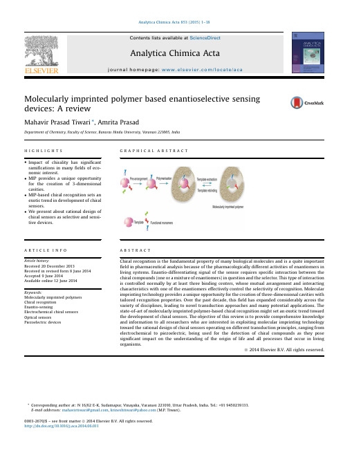
Molecularly imprinted polymer based enantioselective sensing devices: A review
We present about rational design of chiral sensors as selective and sensitive devices.
GRAPArticle history: Received 20 December 2013 Received in revised form 8 June 2014 Accepted 9 June 2014 Available online 12 June 2014
ã 2014 Elsevier B.V. All rights reserved.
* Corresponding author at: N 16/62 E-K, Sudamapur, Vinayaka, Varanasi 221010, Uttar Pradesh, India. Tel.: +91 9450239133. E-mail addresses: mahavirtiwari@, krineshtiwari@ (M.P. Tiwari).
毫米波大规模MIMO无线传输关键技术

毫米波大规模MIMO无线传输关键技术尤力;高西奇【摘要】Millimeter wave massive multiple-input multiple-output(MIMO) wireless transmission is a promising technology for future wireless communications as it can expand the use of new spectrum resources, efficiently exploit the space domain wireless resources, and significantly improve the wireless data transmission rate. Based on the millimeter wave massive MIMO architecture, this paper presents a brief overview of the key techniques in millimeter wave massive MIMO wireless communications, including channel modeling, channel information acquisition, multiuser transmissions, and joint resource allocation.%认为毫米波大规模多输入多输出(MIMO)无线传输能够拓展利用新频谱资源,深度挖掘空间维度无线资源,大幅提升无线传输速率,是未来无线通信系统最具潜力的研究方向之一.基于毫米波大规模MIMO无线传输基本架构,论述了信道建模、信道信息获取、多用户无线传输及联合资源调配等毫米波大规模MIMO无线传输关键技术.【期刊名称】《中兴通讯技术》【年(卷),期】2017(023)003【总页数】3页(P11-13)【关键词】大规模MIMO;毫米波通信;信道信息;波束赋形【作者】尤力;高西奇【作者单位】东南大学,江苏南京 210096;东南大学,江苏南京 210096【正文语种】中文【中图分类】TN929.5随着现代信息社会的高速发展,各种移动新业务需求持续增长,无线传输速率需求将继续呈现指数增长趋势。
- 1、下载文档前请自行甄别文档内容的完整性,平台不提供额外的编辑、内容补充、找答案等附加服务。
- 2、"仅部分预览"的文档,不可在线预览部分如存在完整性等问题,可反馈申请退款(可完整预览的文档不适用该条件!)。
- 3、如文档侵犯您的权益,请联系客服反馈,我们会尽快为您处理(人工客服工作时间:9:00-18:30)。
Performance of spatially correlated MIMO channel with antenna selectionL.Y ang,D.Tang and J.QinThe exact bit error rate of a multiple-input multiple output system with transmit antenna selection in a spatially correlated channel is derived.Only one transmit antenna is chosen for transmission.Results show that transmit antenna selection performs considerably worse than full-complexity schemes in completely correlated channels.Introduction:Recently,many papers [1–3]have investigated antennaselection schemes for multiple-input multiple-output (MIMO)systems,but these results are valid for the uncorrelated Rayleigh channels (e.g.IID Rayleigh flat fading channels);no exact expression is available for the correlation case.In this Letter,we consider a system with antenna selection at the transmitter.At any time,only one out of n T transmit antennas is selected and activated for transmission;other transmit antennas are inactive.All the receive antennas are used without selection.The exact bit error rate (BER)of such a scheme for binary phase-shift keying (BPSK)modulation in spatially correlated MIMO channels is presented.System and channel model:We consider a single-user MIMO with n Ttransmit and n R receive antennas.The receiver has perfect channel state information (CSI)and the transmitter has no CSI.The maximum ratio combining (MRC)scheme is applied at the receiver.At any time,only a single transmit antenna is selected and the other antennas are inactive.We adopt the widely used model for the correlated channel model [1]:H ¼R 1=2WT 1=2ð1Þwhere H is the n R Ân T channel matrix,W is a matrix with independentcomplex Gaussian identically distributed entries,and R ,T are n R Ân R ,n T Ân T matrices denoting the receive and transmit correlation matrixes,respectively.Here we consider the semi-correlated Rayleigh channel and assume that the correlation happens at the receiver,so that T is an n T Ân T identity matrix I nT .Using singular value decomposition (SVD),we have R ¼U L V H ,where U ,V are unitary matrixes,L ¼diag[v ],v ¼[v 1,...,v n R ].To fix the average channel transmission power,we assume P i ¼1n R v i ¼n R .BER derivation:Defining a j ¼P i ¼1n Rj h i,j j 2,1 j n T ,which is the instantaneous channel gain between transmit antenna j and all the receive antennas,and assuming a 1 a 2 ...a n T ,at any time,a single transmit antenna corresponding to a S is selected,where S is a fixed integer and 1 S n T .It is obvious that S ¼n T is the best antenna selection since it maximises the total received signal power,so it will be chosen for transmission.The instantaneous signal-to-noise ratio (SNR)per bit g at the output of the MRC combiner can be written asg ¼ga n Tð2Þwhere g ¯¼E b =N 0is the average SNR,E b is the average energy per bit atthe transmitter and N 0denotes the variance of additive white Gaussian noise (AWGN).It is well known that the conditional BER for BPSK isgiven by Q (p (2g¯a n T ));the average BER is obtained from P b ðE Þ¼ð10Q ðffiffiffiffiffiffiffiffiffiffiffi2ga n T q Þp a n Tða n T Þd a n Tð3ÞIn a spatially correlated Rayleigh channel,a j are exponentially distrib-uted random variables;the characteristic function (CF)of a j is given by [4]F ðw Þ¼Qn R i ¼111Àjv i wð4ÞWe can write the probability density function (PDF)of a j asp ðx Þ¼12p ð1À1Q n R i ¼111Àjv i we Àjwx dw x !0ð5Þwe note that (4)can be rewritten asF ðw Þ¼Pn R i ¼1z 1Àjv i wð6Þwhere z ¼Qn R i 0¼1i 0¼1v i =v i Àv 0i :After some manipulation,we can rewrite (5)asp ðx Þ¼P n R i ¼1zexp ðÀx =v iÞv i x !0ð7Þand the cumulative density function (CDF)of a j is given byP ðx Þ¼P n R i ¼1z ð1Àe Àx =v i Þx !0ð8ÞThe PDF of a n T can be found in [5]:p a n Tðx Þ¼n T ½P ðx Þ n T À1p ðx Þð9ÞSubstituting (7)and (8)into (9),we havep a n T ðx Þ¼n T P n R i ¼1z ð1Àe Àx =v iÞ n T À1P nR i ¼1z exp ðÀx =v i Þv i ð10ÞFrom (10),we can rewrite (3)asP b ðE Þ¼ð10Q ðffiffiffiffiffiffiffi2g x p Þn T P nR i ¼1z ð1Àe Àx =v iÞ n T À1P n R i ¼1z exp ðÀx =v i Þv i dx ð11ÞAfter some manipulation,we can rewrite (11)asP b ðE Þ¼n TP n R i ¼1z i P n T À1k ¼0ðÀ1Þk n T À1k P n R i ¼1z n T À1ÀkÂð10Q ðffiffiffiffiffiffiffi2g x p ÞP nR i ¼1z e Àx =v ik exp ðÀx =v i Þdxð12ÞIn general,the expression in (12)is difficult to analyse directly,and needs a singular numerical integral.Special case:Here we concentrate on the n R ¼2case;the case for n R !3is not practical because it is difficult to distribute more antennas at the mobile set for the downlink communications.Let n R ¼2,from (12),we haveP b ðE Þ¼n TP n T À1k ¼0ðÀ1Þk n T À1k 1ðv 1Àv 2Þk þ1Âð10Q ðffiffiffiffiffiffiffi2g x p Þ½v 1e Àx =v 1Àv 2e Àx =v 2 k ½e Àx =v 1Àe Àx =v 2dxð13ÞThe integral in (13)can be written asð10Q ðffiffiffiffiffiffiffi2g x p Þ½v 1e x =v 1Àv 2e Àx =v 2 k ½e Àx =v 1Àe Àx =v 2 dx ¼P k i ¼0ðÀ1Þi v k Ài 1v i 2k i ð1Q ðffiffiffiffiffiffiffi2g x p Þe À½k Ài þ1=v 1þi =v 2 x dxÀð10Q ðffiffiffiffiffiffiffi2g x p Þe À½k Ài =v 1þi þ1=v 2 xdx ð14ÞAfter some manipulation,we can finally rewrite (13)asP b ðE Þ¼n T v 1v 2P n T À1k ¼0ðÀ1Þk n T À1k 1ðv 1Àv 2ÞP k i ¼0ðÀ1Þi v k Ài 1v i 2k i Â1Àffiffiffiffiffiffiffiffiffiffiffiffiffiffiffiffiffiffiffiffiffiffiffiffiffiffiffiffiffiffiffiffiffiffiffiffiffiffiffiffiffiffiffiffiffiffiffiffiffiffiffiffiffiffiffiffiffiffiffiffiffiffiffiffiffiffiffiffiffiffiffiffiðv 1v 2 gÞ=ðv 2ðk Ài þ1Þþiv 1þv 1v 2 g Þp v 2ðk Ài þ1Þþiv 1(À1Àffiffiffiffiffiffiffiffiffiffiffiffiffiffiffiffiffiffiffiffiffiffiffiffiffiffiffiffiffiffiffiffiffiffiffiffiffiffiffiffiffiffiffiffiffiffiffiffiffiffiffiffiffiffiffiffiffiffiffiffiffiffiffiffiffiffiffiffiffiffiffiffiffiffiffiðv 1v 2 gÞ=ðv 2ðk Ài Þþði þ1Þv 1þv 1v 2 g Þp v 2ðk Ài Þþv 1ði þ1Þ)ð15ÞTherefore,the BER for the spatially correlated Rayleigh channel with transmit antenna selection is written in concise closed form.Next we consider two special cases:one is the completely uncorrelated case,the other is the completely correlated case.For the completely uncorrelated case,we know that T ¼R ¼I ,v 1¼v 2¼1,in this case,a j areELECTRONICS LETTERS 30th September 2004Vol.40No.20chi-squared variables with2n R degrees of freedom.The BER for this case can be computed in closed form(note this result is similar to[2]):P bðEÞ¼n T4P n TÀ1k¼0ðÀ1Þkðn TÀ1Þ!ðkþ1Þ2k!ðn TÀ1ÀkÞ!ÂP kt¼0ðtþ1Þk!½2ðkþ1Þ tðkÀtÞ!1Àffiffiffiffiffiffiffiffiffiffiffiffiffiffiffiffiffiffiffigs!tþ2ÂP tþ1j¼02Àjðtþjþ1Þ!1þffiffiffiffiffiffiffiffiffiffiffiffiffiffiffiffiffiffiffigs!j359=;ð16ÞFor the completely correlated case,we have v1¼2,v2¼0.The BER for this case is given byP bðEÞ¼n T2P n TÀ1k¼0ðÀ1Þkðn TÀ1Þ!k!ðn TÀ1ÀkÞ!ð1Qðffiffiffiffiffiffiffi2 g xpÞeÀðkþ1Þx=2dxð17ÞThe evaluation of(17)needs some variable transform;finally we can obtainP bðEÞ¼n TP n TÀ1k¼0ðÀ1Þkðn TÀ1Þ!T1Àffiffiffiffiffiffiffiffiffiffiffiffiffiffiffiffiffiffiffiffiffi2 gs"#ð18ÞFig.1Comparison of analytical and simulated BER for spatially corre-lated MIMO channels with different levels of correlation,BPSK———analytical:v1¼2,v2¼0*simulation:v1¼2,v2¼0———analytical:v1¼1.6,v2¼0.4s simulation:v1¼1.6,v2¼0.4–—–—analytical:v1¼v2¼1u simulation:v1¼v2¼1–—*–—no antenna selection:v1¼2,v2¼0Performance:In Fig.1,the analytical and simulated BER results arecompared with n T¼2,n R¼2;only one transmit antenna is chosen.Wefind that the analytical resultsfit the simulated curves correctly.FromFig.1we observe that the correlation at the receiver can reduce theperformance,in completely correlated channels;the transmit antennaselection performs considerably worse than full-complexity schemes.#IEE200411June2004Electronics Letters online no:20045802doi:10.1049/el:20045802L.Y ang, D.Tang and J.Qin(Department of Electronics andCommunication Engineering,Sun Yat-sen University,510275,Guangzhou,China)References1Molisch,A.F.,and Zhang,X.:‘FFT-based hybrid antenna selectionschemes for spatially correlated MIMO channels’,IEEE Commun.Lett.,2004,8,pp.36–382Chen,Z.,et al.:‘Analysis of transmit antenna selection=maximal-ratiocombining in Rayleigh fading channels’.Proc.ICCT2003—Int.Conf.on Communication Technology,Beijing,China,April2003,V ol.2,pp.1532–15363Molisch,A.F.,and Win,M.Z.:‘MIMO systems with antenna selection’,IEEE Microw.Mag.,2004,pp.46–564Proakis,J.G.:‘Digital communications’(McGraw-Hill,New Y ork,USA,2001)5/OrderStatistic.htmlELECTRONICS LETTERS30th September2004Vol.40No.20。