
FDTD_solutions操作案例1
以上面图像为例子,设置时只需要设置一个周期,然后将边界设为周期结构即可。
1.打开fdtd软件
2.单击structures设置结构。
3.选中物体单击右键设置参数。
给结构命名,x,y,z确定结构在各个方向上的范围。
5设置选中结构的材料,如果material里有想要的材料直接选中即可,没有的可以通过查询,将其折射率直接输入到index中。
6.当结构重叠时,可勾选下面按钮,设置重叠部分的优先性,数字越小优先性越高。
7.设置基底上的光栅结构,先设置下层Al。
8.设置中间层PMMA
9.设置上层Al
10.单击Simulation选中region设置模拟区域。
Geometry设置单元结构参数,一般选取一个周期即可,所以X span和Y span就是周期,然后在boundary conditions中将x,y都选为periodic。
点击OK.
11.在Source中选取plane wave,genaral中入射方向改为向下入射,geometry中X span和Y span选取的要比周期大,Frequency/wavelength中改变入射波长范围。
12.在Monitor中选取frequency domain field and power探测器。
勾选第一项,将frequency points变为200,将探测器放于光源上方探测反射率。
还可以在选取一个探测器放于下方探测投射,一次模拟可以放入多个探测器。
13.结构设置完成之后,点击RUN,运行,待运行完毕后,选择对应的探测器,可以看出探测到的结果。
FDTD软件介绍及案例分析一

比较模拟性能的理想化设备相对的装置,就能制造的——在 这儿,把表面粗糙度测量通过原子力显微镜的测量——可以帮 助找出在设计和生产过程的设备性能改善的好处。
11
CMOS图像传感器像素设计
12
CMOS图像传感器像素设计
14
CMOS图像传感器像素设计
• 第三步:优化角度回应的CMOS图像传感器和测量主要射线 角度:增加光学效率、降低光谱光相声
测量光谱光相声,向下的功率流在邻近的sub-pixels可以 计算,结合矢量。光谱光相声一般产生最小光学效率最大化, 但在陡峭的角度入射高浓度的相声观察到,在某种程度上,不 可避免的。更复杂的装置设计,由其他的像素元素(如互连) 也改变时,可以提供一种方法,可以减少整体相声水平。
FDTD Solutions 帮助 _ Quality factor calculations
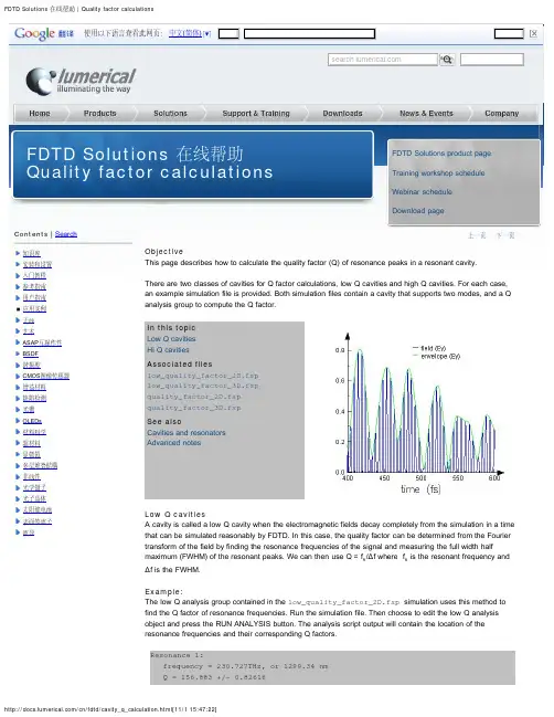
知识库安装和设置入门教程参考指南用户指南应用实例天线艺术ASAPBSDF谐振腔CMOS增益材料缺陷检测光栅OLEDs材料科学超材料显微镜多层堆叠結構非线性光学镊子光子晶体太阳能电池表面等离子波导A cavity is called a low Q cavity when the electromagnetic fields decay completely from the simulation in a timeFDTD Solutions 在线帮助Quality factor calculations FDTD Solutions product page Training workshop schedule Webinar schedule Download page)SearchResonance 2:frequency = 205.814THz, or 1456.62 nmQ = 77.498 +/- 0.226738The analysis script also creates two plots. The plot shown below to the left contains one of the field components (Hz). You can see that the fields have decayed by the end of the simulation time. The second plot shows the location and relative amplitude of the resonance peaks.Note that the initial transients of the source are neglected by setting the "start time" for the time monitors to 200fs. The "start time" for the time monitors is the time at which the monitors begin recording data. This setting can be changed in the user properties for the analysis group. Also, note that in the analysis group, it is possible to use one time monitor or an array of time monitors for the Q factor calculation. The problem with using one time monitor is that if the one monitor is placed at or near a null of the cavity mode, then due to the fact that the field intensity is very low, the Q factor can have a large uncertainty (if it is even possible to obtain a meaningful result).The low_quality_factor_3D.fsp simulation file contains a 3D version of the low Q analysis object.High Q cavitiesA cavity is considered to be a high Q cavity when the electromagnetic fields cannot completely decay from the simulation in a time that can be simulated reasonably by FDTD. In this case, we cannot determine Q from the frequency spectrum because the FWHM of each resonance in the spectrum is limited by the time of simulation,Tsim , by FWHM ~ 1/Tsim. Instead, the quality factor should be determined by the slope of the envelope of thedecaying signal using the formulawhere fRis the resonant frequency of the mode, and m is the slope of the decay in SI units.Derivation of Q factor formula:The quality factor (Q) is defined aswhere wris the resonant frequency and FWHM is the full width half max of the resonance intensity spectrum. The time domain signal of the resonance is described bywhere α is the decay constant. The fourier transform of E(t) is easy to calculate.The maximum value of |E(w)|^2 is clearly 1/α^2, at w=wr. With a little more work, we can determine that thehalf max frequencies occurs at w=wr + α and w=wr- α. Therefore, FWHM = 2α. Substituting this value intothe original Q formula and solving for α givesNow that we know how to relate α to Q, we must determine how the slope of the time signal decay is related to Q. We must take the log of the time signal to make the envelope a linear function.where m is the slope of the log of the time signal envelope. Solving for Q, we get.Example:Calculation of the Q factor for high Q cavities is complicated because•separating the decay of the envelope from the underlying sinusoidal signal is difficult since the fields are typically real-valued•if there are multiple resonant modes, they will interfere with each other in the time domain, making it hard to estimate the decay rate.By opening the edit dialog box for the Q factor analysis object located in quality_factor_3D.fsp, you can see that the analysis object solves these problems by•accurately calculating the envelope of the time-domain field signal•isolating each resonance peak in the frequency domain using a Gaussian filter, and then taking the inverse Fourier transform to calculate the time decay separately for each peak. The slope of the time decay is then used to calculate the Q factor and obtain an error estimate.In addition, note that:•the Q analysis object has setup variables that allow you to choose how many time monitors to use to calculate the Q factor. It is often a good idea to add a few point monitors at different locations to reduce the chances that a monitor is placed at a node in the mode profile of a cavity mode yielding a weak signal.•in the analysis tab, there is a parameter that can be set to choose how many resonant peaks to look for •all the field components that are available are used to calculate the Q factor•it is possible to change other parameters, such as the Gaussian filter width and resolution in the frequency domain. These parameters are set in the analysis script.•in the script, only the part of the time signal lying in 40-60% of the time signal collected is used for the slope calculation. These percentages can easily be changed. However, setting the upper limit to anything greater than 90% can lead to errors due to the fact that Fourier transforms, and inverse transforms were used when the Gaussian filter was used to isolate the peak. The Fourier transforms introduce errors to the end of the time signal due to the fact that discrete Fourier transforms assume periodicity of the signal.Next, run the simulation. When the simulation is complete, choose to edit the analysis object and press RUN ANALYSIS button. The analysis script output will contain the location of the resonance frequencies and their corresponding Q factors.Resonance 1:frequency = 178.786THz, or 1676.82 nmQ = 306.279 +/- 1.41318Resonance 2:frequency = 227.307THz, or 1318.89 nmQ = 274.874 +/- 4.50921The analysis object also produces the following plots.The time decay of the field components and their envelopes. Note The spectrum and the Gaussian filtersThe spectrum of resonances. Each resonant peak appears in a The time decay of the sum of squared Other versions of this page:Events。
FDTD操作案例
一基于A u薄膜正三角形孔阵列提取光场强度分布图本例子中取Au薄膜厚度30nm,三角形孔阵周期800nm,小孔直径600nm。
Au的材料模型选取“Au (Gold)–CRC”,或者自建材料模型。
参见hole arrays_E fied 文件。
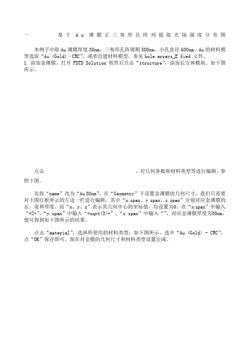
1.添加金薄膜,打开FDTD Solution 软件后点击“structure”,添加长方体模块。
如下图所示。
点击,对几何参数和材料类型等进行编辑。
参照下图。
先将“name”改为“Au 30nm”,在“Geometry”下设置金薄膜的几何尺寸,我们只需要对下图红框所示的左边一栏进行编辑,其中“x span、y span、z span”分别对应金薄膜的长、宽和厚度,而“x、y、z”表示其几何中心的坐标值,均设置为0。
在“x span”中输入“*2+”,“y span”中输入“*sqrt(3)+”,“z span”中输入“”,对应金薄膜厚度为30nm,便可得到如下图所示的结果。
点击“material”,选择所使用的材料类型,如下图所示,选中“Au (Gold) - CRC”,点“OK”保存即可。
现在对金膜的几何尺寸和材料类型设置完成。
2.在金薄膜中添加小孔阵列。
点击中的三角形,在下拉菜单中选择“Photonic crystals”。
然后在屏幕右侧的“Object”一栏中选中“Hexagonal lattice PC array”,点击“Insert”进行添加。
在左侧的结构树“object tree”中选中“hex_pc”,即我们刚才添加进去的六边形阵列,点击对它进行编辑。
各参数设置如下图所示,其中“a”表示小孔之间的间距,即三角形孔阵的周期,“radius”表示小孔半径。
设置完成后,点“ok”保存。
经过上面的步骤,我们搭建的模型的如下图所示。
我们发现经过上面的设置所得到的三角形孔阵列其中两个小孔超出了金膜,为了好看起见,希望将多余的这两个小孔删掉,首先,如下图所示,在结构树下选中“hex_pc”,单击鼠标右键在菜单中选择“break groups”,不进行这项操作无法删掉多余的小孔。
FDTD操作案例2
一基于AU 薄膜正三角形孔阵列提取光场强度分布图本例子中取AU薄膜厚度30nm ,三角形孔阵周期800nm,小孔直径600nm。
AU的材料模型选取"AU (Gold) - CRC ”,或者自建材料模型。
参见hole arrays_E fied Profile.fsp文件。
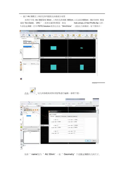
1.添加金薄膜,打开FDTD Solution软件后点击“StrUCtUre”,添加长方体模块。
如下图所示。
IVn Ala e⅛ιl 先将“ name'改为“ AU 30nm”,在“ Geometry”下设置金薄膜的几何尺寸, IiJul ÷lF-I♦ < * ∙T wWModel• ITrtBPgle⅛C⅛∏fl⅛■1III__________ _ ”对几何参数和材料类型等进行编辑。
参照下图。
⅜•*4 ,□ T/** 迦^⅞4 ・⅝ ▼B ∙βilcrτ 门零S⅞j⅛c⅞urts ftttribnUi CwfOMntE ⅛f OTflIS ArllIyEi ιI*P4iFt Scnurcis两In £灯E BtE4TKf<!⅛G ct⅞⅛HLame⅛* m□t⅛lιA<lpr⅛∣lririlMame-DimefISECIm∕⅛akIB.■Iy XJ-Iripa-ClLm Ti.I oll I JllrStE Tr-Iril;2寻XFnD LTKau⅛Dlm» & o M点击T J-∣4XT TIrR 5⅛-jp∣KS 址Farl l H⅞UVl VL*τRιτul LTIrH我们只需要对下图红框所示的左边一栏进行编辑,其中“X SPan、y SPan、z SPan” 分别对应金薄膜的长、宽和厚度,而“ x、y、z”表示其几何中心的坐标值,均设置为0。
在“X span” 中输入“0.8*2+0.6 ”,“y SPan” 中输入"0.8*sqrt(3)+0.6 ”“Z SPan ”中输入“ 0.03 ”,对应金薄膜厚度为30nm便可得到如下图所示的结果。
FDTD Solutions—专业的微纳光学仿真软件

2012 2011 2010
2008
2006 2005 2004 1998
1.上海海基盛元 — 公司文化
共享成功
社会责任
真诚服务
幸福快乐
7 软件商城:/ (各类科研与工程软件)赵海军:136 4166 4322
自适应网格 简化的监视器获得输出数据 利用覆盖区减少网格点数
• 仿真速度快(最快)
超短的脉冲光源 需要的内存少 并行计算
• 结果精确
多系数材料建模 共形网格技术
• 可以仿真各种材料:介质,金属,半导体,非线性,各向异性,增益 • 其它特点
15 软件商城:/ (各类科研与工程软件)赵海军:136 4166 4322
包含扫描与优化 ……
4.特点优势 — FDTD Solutions 8.0最新功能
1)用户可以自定义色散材料、增益材料、各向异性材料和非线性材料
:非对角各向异性材料,包括液晶材料和磁光材料 :含内嵌的x(2)材料和顺磁性材料
2)改变了分析和视觉化工具
:增加了结果管理器Results Manager, 可以直接观看结果数据 :增加了视觉化器Visualizer, 可以用于图示分析 :数据可以保存在监视器里面
上海总部
华南办事处
无锡东方海基软件开发有限公司
3 软件商城:/ (各类科研与工程软件)赵海军:136 4166 4322
1.上海海基盛元 — 理念与使命
理 念
国内领先的专业工程软
件、管理软件以及服务 的提供商
使 命
提供行业领先的仿真分 析以及信息化管理的解 决方案,从而帮助客户 提高产品研制水平、缩 短产品研制周期、降低 产品研制费用,使其在 激烈的产品竞争中处于 领先地位
FDTD使用
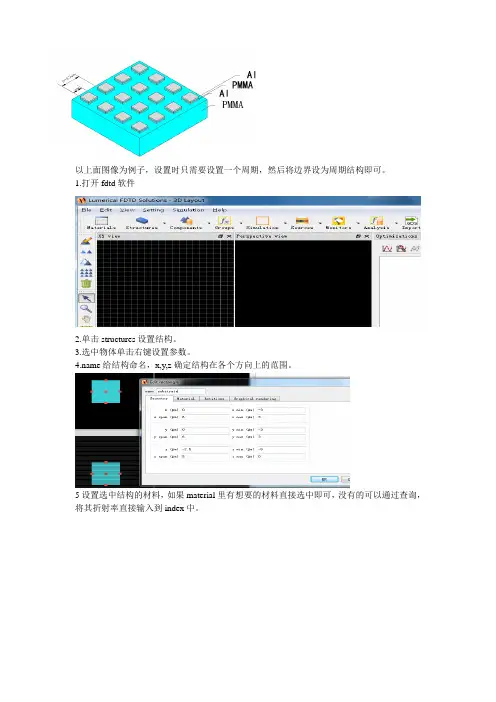
以上面图像为例子,设置时只需要设置一个周期,然后将边界设为周期结构即可。
1.打开fdtd软件
2.单击structures设置结构。
3.选中物体单击右键设置参数。
给结构命名,x,y,z确定结构在各个方向上的范围。
5设置选中结构的材料,如果material里有想要的材料直接选中即可,没有的可以通过查询,将其折射率直接输入到index中。
6.当结构重叠时,可勾选下面按钮,设置重叠部分的优先性,数字越小优先性越高。
7.设置基底上的光栅结构,先设置下层Al。
8.设置中间层PMMA
9.设置上层Al
10.单击Simulation选中region设置模拟区域。
Geometry设置单元结构参数,一般选取一个周期即可,所以X span和Y span就是周期,然后在boundary conditions中将x,y都选为periodic。
点击OK.
11.在Source中选取plane wave,genaral中入射方向改为向下入射,geometry中X span和Y span选取的要比周期大,Frequency/wavelength中改变入射波长范围。
12.在Monitor中选取frequency domain field and power探测器。
勾选第一项,将frequency points变为200,将探测器放于光源上方探测反射率。
还可以在选取一个探测器放于下方探测投射,一次模拟可以放入多个探测器。
13.结构设置完成之后,点击RUN,运行,待运行完毕后,选择对应的探测器,可以看出探测到的结果。
FDTD案例分析续篇
11
纳米粒子散射
12
实例二 :纳米线栅偏振器
1、纳米线网格偏振镜紧凑光子偏振控制元素——与解决方 案设计和优化FDTD • 高对比度极化控制装置的组成sub-wavelength金属光栅纳米线偏振器件——正在取代网格批量光学元素。纳米线 网格偏振器件提供改进消光比对比,最小的吸收来解决高 亮度照明,紧凑的形式因素促进大规模生产和集成在小型 光学组件。然而,纳米线偏振器件是富有挑战性的网格组 件来设计,特别是如果制造缺陷都考虑进去。在这个应用 程序中,我们将展示FDTD解决方案可以用来最大化对比度 的纳米线偏振镜网格任意角度,同时保持高传播。
33
SPR纳米光刻
• 第三步:分析了表面等离子体共振光刻近场数据 详细的研究结果和数值的解决方案,所有复杂的光学波的 交互的接口的许多材料,包括硅基片上的反射,准确地对待。 一个阴谋的近场强度在截面通过银丝面膜层(y=0到60海里) 和光刻胶层(y = -50到0 nm)显示在对数。表面等离子体模 式是清楚地看到在银胶面罩/接口。周期性结构允许入射光 束夫妇counter-propagating表面等离子体波,这引起了亚波 长的变化在光阻层强度的设计思想。
18
纳米线栅偏振器
19
纳米线栅偏振器
• 第四步:模拟得到的响应非正态纳米线网格发病率照明。 铝光栅wiregrid偏振镜有TE传播的大约85%的normallyincident平面波。现在,与一个源呈四十五度角,传播下降到 大约83%。这些结果生成模拟一个时期的wiregrid偏振镜,然 后使用复杂的脚本的环境,在解决方案将FDTD响应从单个光 栅牙的反应,multi-tooth组成部的铝光栅。
36
FDTD Solutions资料集锦专题资料(一)
如何成功完成您的Lumerical注册.pdf
算例下载区:
谐振腔相关算例:
FDTD案例-谐振腔-光学晶子.rar
FDTD案例-谐振腔-quality_factor.rar
FDTD案例-谐振腔-低质因子.rar
FDTD案例-谐振腔-型腔回音壁.rar
FDTD案例-谐振腔-PC_3D.rar
FDTD案例-谐振腔-型腔模振幅.rar
克斯普朗克研究院、麻省理工学院、美国国家标准与技术研究院、东京大学
、清华大学、北京大学和中国科学院多个研究所等,都在使用Lumerical的设 计软件软件。
FDTD参考手册
Lumerical 2014a安装手册.pdf
Lumerical Flexnet code license安装步骤(最新).pdf
FDTD Solutions资料集锦 专题(一)
更新时间:2015-2-4
以下是小编整理的一些FDTD Solutions资料集锦,其中包括了有关FDTD
Solutions FDTD参考手册、应用算例。有关文档的下载,可以到研发埠 网站的专题模块,输入相应的Байду номын сангаас题名,搜索到相应的专题便可以找学软件 FDTD Solutions
FDTD Solutions软件由加拿大Lumerical Solutions公司出品。通过向研究和 产品开发专业人士提供基于计算技术最新发展的高性能光学设计软件, Lumerical帮助光学设计者达到挑战性设计目标,满足严格的设计期限要求。 Lumerical的设计软件已在 30多个国家应用,全球科技领先厂商,如安捷伦 、ASML、博世、佳能、Harris、Northrop Grumman、奥林巴斯、飞利浦、三 星和意法半导体,以及众多卓越研究机构,如哈佛大学、加州理工学院、马
微纳光子学设计分析软件FDTD Solutions专题资料集锦(四)
Numerical study of natural convection in porous media (metals) using Lattice Boltzmann Method (LBM).pdf 自然对流多孔介质(金属)用晶格玻尔兹曼方法加快的数值研究 A thermal lattice BGK model with doubled populations is proposed to simulate the two-dimensional natural convection flow in porous
金属/半导体核壳结构电浆子模式研究
The symmetry-broken geometry and variation of metal composition of semishells induce new plasmonic properties. A system of separated
metallic semishells embedded in a poly(dimethylsiloxane) polymer
and porosity on the natural convection are examined. Also the
effect of porous media configuration (shape) on natural convection is investigated. The results showed that the overall heat transfer
structure obtained by spinodal decomposition. Its optical response
was investigated both experimentally and theoretically. Our results show that this structure has interesting optical properties due to the existence of only short-range order and the lack of welldefined local structures.
FDTD入门教程
欢迎进入FDTD Solutions 的入门教程!入门教程由四章内容组成。
第一章介绍FDTD Solutions 的基本功能,以及器件建构,程序运行和结果分析。
后面三章则针对v个实际问题,提供详细指导,帮助用户一步步地了解每一模块的功能及其使用。
文中涉及的所有模拟设计文件都可以从LUMERICAL 的相应网页上免费下载。
第一章简介第二章银质纳米线谐振腔散射教程第三章环形谐振腔教程第四章光子晶体微腔教程简介The goal of the Getting Started Guide is to introduce the Finite Difference Time Domain (FDTD) technique and explain how modeling is done with the software.The FDTD algorithm is useful for design and investigation in a wide variety of applications involving the propagation of electromagnetic radiation through complicated media. It is especially useful for describing radiation incident upon or propagating through structures with strong scattering or diffractive properties. The available alternative computational methods - often relying on approximate models - frequently provide inaccurate results. FDTD Solutions is useful for numerous engineering problems of commercial interest including:• display technologies• optical storage devices• LED design• biophotonic sensors• plasmon polariton resonance devices• optical waveguide devices• photonic crystal devices• integrated optical filters• optical micro cavity designFDTD Solutions is an accurate and easy to use, versatile design tool capable of treating this wide variety of applications. This introductory chapter of the Getting Started Guide introduces the general FDTD method and provides a basic overview of the product usage. The final sections contain examples that are accompanied by step-by-step instructions so that you can set up and run the simulations yourself.什么是时域有限差分?The Finite Difference Time Domain (FDTD) method has become the state-of-the-art method for solving Maxwell’s equations in complex geometries. It is a fully vectorialmethod that naturally gives both time domain , and frequency domain information to the user, offering unique insight into all types of problems and applications inelectromagnetics and photonics .The technique is discrete in both space and time . The electromagnetic fields and structural materials of interest are described on a discrete mesh made up of so-called Yee cells . Maxwell’s equations are solved discretely in time, where the time step used is related to the mesh size through the speed of light. This technique is an exactrepresentation of Maxwell’s equations in the limit that the mesh cell size goes to zero. Structures to be simulated can have a wide variety of electromagnetic material properties. Light sources may be added to the simulation. The FDTD method is used to calculate how the EM fields propagate from the source through the structure . Subsequent iteration results in the electromagnetic field propagation in time. Typically, the simulation is run until there are essentially no electromagnetic fields left in the simulation region.Time domain information can be recorded at any spatial point (or group of points). This data can be recorded for the duration of the simulation, or it can be recorded as a series of "snapshots" at times specified by the user.Frequency domain information at any spatial point (or group of points) may be obtained through the Fourier transform of the time domain information at that point. Thus, the frequency dependence of power flow and modal profiles may be obtained over a wide range of frequencies from a single simulation.In addition, results obtained in the near field using the FDTD technique may be transformed to the far field, in applications where scattering patterns are important.More information about the FDTD method, including references, can be found in the Physics of the FDTD Algorithm section of the reference guide.FDTD的用户界面This section discusses useful features of the FDTD Solutions Graphical User Interface (GUI).In this topicGraphical User Interface: Windows andToolbarsAdd Objects to the simulationEdit ObjectsStart a new 2D/3D simulationGraphical User Interface: Windows and ToolbarsThe graphical user interface contains useful tools for editing simulations, including• a toolbar for adding objects to the simulation• a toolbar to edit objects• a toolbar to run simulations•an objects tree to show the objects which are currently included in the simulation• a script file editor window•an object library• a window to set up parameter sweeps and optimizationsIn the default configuration some of the Windows are hidden. To open hidden windows, click the right mouse button anywhere on the main title bar or the toolbar to get the pop up window shown in the screen shot below. The visible windows/toolbars have a check mark next to their name; the hidden ones do not have check marks. A second way to obtain the pop up window is to go to the main title toolbar and select VIEW->WINDOWS.For more information about the toolbars and windows see the Layout editor section of the reference guide.Add Objects to the simulationThe Graphical User interface contains buttons to add objects to the simulation. Click on the arrow next to the image to get a pull down menu which shows all the available options in a group. The screenshot below shows what happens when we click on the arrow next to the COMPONENTS button. Note that the picture on the button is the same as the MORE CHOICES option in the list. If we click on the button itself (instead of the arrow) we will go directly to the MORE CHOICES section of the object library.Also notice that the picture for the COMPONENTS button will change depending on what the last component that was added to the simulation was. Finally, the ZOOM EXTENTbutton in the toolbar will resize the viewports to fit all the objects currently included in the simulation.Edit objectsTo edit an object, select the object and press E on the keyboard or press the EDIT buttonon the toolbar. The easiest way to select an object is to click on the name of the object in the objects tree. However, objects can also be selected by clicking on the graphical depiction of them when the SELECT button is pressed. For more information see the Layout editor section of the reference guide.When we edit objects in FDTD, we get an edit window. The edit windows have units for the settings; in the GEOMETRY tab, the x, y and z location will be in μm by default. The units can be changed to nm if we choose SETTINGS->LENGTH units in the main menu. Fields in the edit windows act like calculators, so that equations can be entered in the fields. See the y span field below for an example.Start a new 2D/3D simulationBy default FDTD Solutions opens with a blank 3D simulation. In the following Getting Started Examples, we often begin with a 2D simulation, which can be obtained as shown in the screenshot below.模拟运行与优化This section discusses important checks which should be made before running a simulation (memory requirements, material fits) and gives links to more information about running simulations and parameter sweeps or optimizations.In this topicCheck memory requirementsCheck material fitsSetup parallel optionsRun simulationRun parameter sweeps and optimizationsCheck memory requirementsTo check the memory requirements, press the CHECK button If this is not the current icon, you can find it by pressing the arrow. Note that the memory report indicates the amount of memory used by each object in the simulation project as well as the total memory requirements. This allows for judicious choice of monitor properties in large and extensive simulations.Check material fitsThe CHECK button also contains a material explorer option . Many of the materials used in FDTD Simulations come from experimental data (see the materials section of the Reference Guide for references for the material data and descriptions of the FDTD material models). Before running a simulation, FDTD Solutions automatically generates a multi-coefficient model fit to the material data in the wavelength range for the source. It is a good idea to check and optimize the material fit before running a simulation. Setup the resource configurationBefore running any simulations, the resource options must be set up. These options canbe accessed by pressing the Resources button . In most cases, the default settings should be fine. The 'number of processes' is typically set to the number of cores in your computer.Run simulationYou can run simulations by pressing the RUN button on the mail toolbar. For more details, such as how to run multiple simulations in distributed mode, please see the RunSimulations section in the online User Guide, or the Running simulations and analysis section of the Reference Guide.Run parameter sweeps and OptimizationsFDTD Solutions also has a built in parameter sweep and optimization window. This window can be seen at the top of the page, and can be opened using the instructions in the Graphical User Interface discussion just prior to this topic.Optimization Window includes buttons to add a parameter sweep and add an optimization. Parameter sweeps and optimizations can include multiple parameters, or be nested. Each optimization or sweep can be run by pressing the right-most button.仿真数据分析This section discusses the tools used to analyze simulation data: the Analysis Window, the script environment and data export to third party software such as MATLAB. For more details please see the Analysis tools and the Scripting language chapters in the Reference Guide.In this topicAnalysis windowScriptingData exportAnalysis windowThe screen shot below shows the open analysis window. The analysis window can be used to plot monitor data.A variety of monitor data can be plotted via the Analysis window, depending on the monitor type. Spatial refractive index data, field vs time, field vs frequency, fields vs spatial dimensions, and power transmission vs frequency are a few examples. The terminology 'Intensity' indicates a squared quantity. For example, 'E intensity' means |E|^2. 'Ex intensity' means |Ex|^2. Field data from frequency monitors is always plotted as an Intensity. If you want to see the real or imaginary parts of the field, or if you want to obtain phase information, the scripting language will be required.ScriptingFDTD Solutions contains a built in scripting language which can be used to obtain simulation data, and do plotting or post-processing of data. The script prompt can be used to execute a few commands, or the built in script file editor can be used to create more complex scripts.A thorough introduction to the Lumerical scripting language can be found in the Scripting section of the FDTD Solutions online user guide. Definitions for all of the script commands are given in the Scripting language chapter in the Reference Guide.Data ExportFDTD simulation data can be exported into text file format using the analysis window, into a Lumerical data file format (*.ldf) which can be loaded into another simulation, or into a Matlab data (*.mat) file. Instructions for exporting to these file formats can be found in the links under the Scripting section.银质纳米线谐振腔散射教程问题综述当光波入射到金属纳米粒子上时,光与金属表面附近的电荷密度相互作用产生的表面等离子体极化surface plasmon polaritons 扮演着重要角色。