第五章-噪声系数测量
噪声系数的测量方法
噪声系数的测量方法噪声系数是指放大器输入信号与输出信号之间的信噪比的比值。
在电子系统中,噪声系数是衡量放大器噪声性能的重要指标。
下面将介绍几种常用的测量噪声系数的方法。
1.级联噪声法:级联噪声法是最常用的测量噪声系数的方法之一、它利用级联放大器的总噪声系数计算出前面的放大器的噪声系数。
具体的步骤如下:a.在待测放大器之前设置一个已知的参考放大器,并测量此参考放大器的噪声系数。
b.将待测放大器与参考放大器级联,并测量级联放大器的总输入输出电压和噪声功率。
c.利用总放大器的输入输出电压和已知的参考放大器的噪声系数计算出内嵌放大器的噪声系数。
2.可变增益噪声法:可变增益噪声法是另一种测量噪声系数的常用方法。
它通过调整放大器的增益,使其与一个已知参考噪声源声压相等,从而测量出待测放大器的噪声系数。
具体的步骤如下:a.在待测放大器的输入端接入一个参考噪声源,并调整其声压使其与待测放大器的输出噪声相等。
b.测量参考噪声源的声压和待测放大器的输入输出电压。
c.利用已知的参考噪声源的噪声功率和声压计算出待测放大器的噪声功率和噪声系数。
3.热噪声法:热噪声法是一种常用的测量噪声系数的方法,特别适用于宽频带和高频段的放大器。
热噪声法利用了热噪声在环境温度下的特性,通过直接测量输出噪声电压和环境温度来计算噪声系数。
具体的步骤如下:a.测量放大器的输出噪声电压并记录。
b.测量环境温度并记录。
c.利用热噪声公式计算出放大器的噪声功率。
d.利用输入信号和已知的电阻值计算出放大器的输入信号功率。
e.利用已知的输入信号功率和噪声功率计算出放大器的噪声系数。
除了上述传统的测量方法之外,还有一些新的测量噪声系数的方法正在不断涌现,如矢量分析器法、差分噪声法、噪声大师法等。
这些方法在特定的应用场景下有着更高的测量精度和更广的测量范围。
总结起来,测量噪声系数的常用方法有级联噪声法、可变增益噪声法、热噪声法等。
根据不同的应用场景和要求,选择合适的方法来测量噪声系数,有助于评估放大器的噪声性能,进而提高信号传输的质量。
频谱仪测噪声系数测试方法

频谱仪测噪声系数测试方法噪声系数是指在信号传输过程中,信号与噪声的比值,是评估通信系统性能的重要指标之一。
因此,测量噪声系数在通信系统设计和优化中具有重要意义。
本文将介绍一种基于频谱仪的噪声系数测试方法。
一、噪声系数的定义噪声系数是衡量信号传输中信噪比的一种指标,通常用dB表示。
它是指在信号传输过程中,输入端信噪比与输出端信噪比之比,即: Nf = (SNRin / SNRout)dB其中,SNRin是输入信号的信噪比,SNRout是输出信号的信噪比。
噪声系数是一个无单位的数值,它越小,表示信噪比损失越小,系统性能越好。
二、频谱仪测噪声系数的原理频谱仪是一种用于测量信号频谱特性的仪器,它可以将信号分解成频率分量,并显示在频谱图上。
在信号传输过程中,噪声会在各个频率分量上产生,因此通过频谱仪可以直接测量出信号的噪声功率谱密度。
在此基础上,可以计算出输入信噪比和输出信噪比,进而计算出噪声系数。
三、频谱仪测噪声系数的步骤1. 连接设备将频谱仪和被测系统连接,确保信号传输通畅。
频谱仪应该与被测系统在同一电源下,以避免地线干扰。
2. 设置频谱仪参数根据被测系统的信号特性,设置频谱仪的参数。
包括中心频率、带宽、分辨率带宽、平均次数等。
3. 测量被测系统的噪声功率谱密度在频谱仪上选择“功率谱密度”模式,启动测量。
记录下被测系统的噪声功率谱密度。
4. 测量输入信噪比在频谱仪上选择“单次扫描”模式,启动测量。
记录下输入信号的功率和噪声功率谱密度,计算输入信噪比。
5. 测量输出信噪比在频谱仪上选择“单次扫描”模式,启动测量。
记录下输出信号的功率和噪声功率谱密度,计算输出信噪比。
6. 计算噪声系数根据输入信噪比和输出信噪比,计算噪声系数。
公式如下:Nf = (SNRin / SNRout)dB四、注意事项1. 频谱仪的选择应根据被测系统的信号特性和测试需求来确定。
2. 在测量过程中,应注意防止干扰和误差的产生。
如地线干扰、环境噪声等。
《噪声系数和测量》课件

设置测量参数:频率、功率、温度等
记录数据:记录测量得到的噪声系数、频率、功率等数据
连接测量仪器:将信号源、功率计、噪声系数分析仪等连接起来
分析数据:分析噪声系数与频率、功率的关系,得出结论
测量结果分析
噪声系数:衡量信号传输过程中噪声的影响程度
测量方法:使用噪声系数测量仪,测量信号的输入和输出噪声
测量结果:噪声系值,表示信号传输过程中噪声的影响程度
噪声系数的应用:在通信、电子、声学等领域都有广泛的应用
噪声系数的计算公式:噪声系数=输出信号功率/输入信号功率
噪声系数的测量
测量原理
噪声系数的定义:描述信号传输过程中噪声增加的程度
测量步骤:首先设置测量参数,然后输入信号,最后读取输出信号并计算噪声系数
注意事项:测量过程中要保证信号的稳定性和准确性,避免干扰因素影响测量结果
添加标题
添加标题
噪声系数测量设备的智能化和自动化
噪声系数测量技术的不断发展和完善
噪声系数测量标准的不断提高和统一
噪声系数测量技术的应用领域不断扩展,如航空航天、电子通信等
展望
噪声系数测量技术的发展:更加精确、快速、便捷
噪声系数测量设备的发展趋势:智能化、小型化、便携化
噪声系数测量在环保领域的应用:更加广泛,更加重要
测量方法:使用噪声系数测量仪,通过测量输入信号和输出信号的功率比来计算噪声系数
测量设备
声级计:测量噪声的强度和频率
频谱分析仪:分析噪声的频率成分
噪声源定位仪:确定噪声源的位置
噪声剂量计:测量噪声暴露剂量
测量步骤
准备测量仪器:噪声系数分析仪、信号源、功率计等
启动测量:启动信号源,调整功率,观察噪声系数分析仪的读数
噪音系数测量
Technical data is subject to change. Copyright@2004 AgilentFundamentalnoise conceptsHow do wemakemeasurements?What DUTscan wemeasure?What influencesthe measurementuncertainty?What is Noise Figure ?NoiseOutNoise inMeasurement bandwidth=25MHza) C/N at amplifier input b) C/N at amplifier outputNinNoutGa RsTwo examples of Noise FigureExample 1: In a receiver, the LNA is connected to an antenna which points to earth’s atmosphere (290K) and the LNA has 3dB NF and 10dB gain. Noise power at LNA output is: -174+10+3=-161dBm/Hz Example 2: In a transmitter the modulator noise floor is -140dBm/Hz. The modulator output is amplifier by a linear amp with 3dB NF and 10dB gain. Noise power at amplifier output is: -140+10+3=-127dBm/Hz-140dBm corresponds to a noise source with a temperature 700 million K, i.e. DUT input is not Standard Temperature and Example 2 is wrongJust to emphasize this point, noise figure only represents the noise added to the input noise referred to the DUT output when the noise into the device is thermal noise at the standard temperature. So the first example here is correct. In the second example, the noise going into the device is much higher and therefore the noise figure of the amplifier cannot be added to the noise out of the DUT from the modulator. In reality if the noise of the amplifier is only 3dB then it will add practically no noise to that generated by the modulator.11An Alternative Way to Describe Noise Figure: Effective Input Noise TemperatureNinNout = Na + kTB GaRsOutput PowerGa , NaSlope=kBGac isti ter c arais NoC ree eFhNa -Te Te Source Temperature (K)Let’s now plot the output noise power as a function of the temperature of the noise source. In the equation for Nout I have substituted Nin for kTB where T now varies from absolute zero upwards. It’s a linear curve as we are dealing with very low power levels so all devices are operating in their linear regions. Actually the line is a very standard ‘y=mx+C’. M is the gradient in this case kBGa and c is the point at which the curve intersects the y axis. C is equal to Na. What you can say at T=0 is that no power at the device output comes from the noise source. All the output power at this point is generated within the DUT. This gives us another figure of merit for describing the noise performance of active devices. If you look at the graph I have drawn the characteristic of a noise free device. If you transpose the added noise Na through this line on to the x axis you arrive at Te, the effective input noise temperature. When you multiply Te by the gain bandwidth product of the device you get the amount of noise added. It’s a useful figure of merit because it is independent of the device gain (unlike Na).12Effective Noise Temperature relation to NFNa + kToBG F= kToBG = Therefore Te = (F-1) . To Na Assume Na = 0 Ts Te kGBTe + kGBTo kBGTo = Te + To ToTsGain GGain GWhat is Te if the NF is 3dB?13Te or NF: which should I use?•Use either - they are completely interchangeable •typically NF for terrestrial and Te for space •NF referenced to 290K - not appropriate in space •If Te used in terrestrial systems and the temperatures can be large (10dB=2610K) •Te is easier to characterize graphically14Friis Cascade FormulaGa1Ga2F1 F2-1 Ga1F2Σ FN+1 = Σ Fn + Fn+1 - 1 ΣGNF12 = F1 +Where Σ Fn is cumulative NF up to nth stage and Σ FN+1 is cumulative NF up to (n+1)th stageNoise figure can be used for much more than just characterizing a single stage. If you know the noise figure and gain of each stage you can calculate the noise figure of a cascade of devices. This equation is known as the cascade formula or Friis formula. F12 is the noise figure of the 2 stage system. G1 is the gain of the first stage, F1 is the NF of the first stage and F2 is the NF of the second stage. The formula clearly shows why you must put your best noise figure devices at the front of the chain. Also the higher the gain of the first stage, the less the noise figure contribution from subsequent stages.15Receiver Modelling using Excelstage 1 stage 2 stage 3 stage 4 TOTAL NF AMP1 2.00 14.00 2.00 14.00 AMP1 2.00 9.00 AMP2 4.00 16.00 2.00 9.00 AMP2 4.00 16.00 2.16 30.00 AMP3 5.00 20.00 2.49 25.00 AMP3 5.00 20.00 2.17 50.00 AMP4 10.00 30.00 2.51 45.00 AMP4 10.00 30.00 2.171NF gain cummulative NF cummulative gain1 22 3 4NF gain cummulative NF cummulative gainstage 1stage 2stage 3stage 4TOTAL NF 2.51NF gain cummulative NF cummulative gainAMP1 4.00 16.00 4.00 16.00 LOSS1 4.00 -4.00 4.00 -4.00AMP2 2.00 14.00 4.03 30.00 AMP1 2.00 14.00 6.00 10.00AMP3 5.00 20.00 4.03 50.00 AMP2 4.00 16.00 6.16 26.00AMP4 10.00 30.00 4.03NF gain cummulative NF cummulative gainAMP3 5.00 20.00 6.1710*LOG((10^(F22/10))+(10^(G20/10)-1)/10^(F23/10))Here is an example of how useful the cascade formula is in the estimation of receiver sensitivity. I’ve used EXCEL to illustrate the example as EXCEL is a very simple and powerful way of performing linear calculations. Both examples have four system components. In the first one I have my low noise amplifier at the front followed by a linear gain block followed by 2 further gain stages. My best noise figure device is placed first as it will dominate the noise figure performance of the system. You can see that the overall noise figure performance is little more than the noise figure of the first stage. The second example is identical, except for the fact that the LNA has lower gain. This mean that the noise contribution of the following stages is more noticeable. The point to make here is that the noise figure of a device is important - but so is its gain. In the third one I have swapped the first two amplifiers around and you can see the difference his has made to the overall noise figure - although the cumulative gain is the same the noise figure is dominated by the first - and now poorer - noise figure performance. The last example is similar to the very fist one except that now4 dB of loss have been introduced. This is common in receiver systems and could represent the cabling between an antenna and the LNA or a front end duplexer. The noise figure of a passive lossy device is equal to its loss. Overall you just add front end losses to the system noise figure to get the overall noise figure The noise figure of a passive device can be seen to be same the magnitude of the insertion gain. For example, a 6dB attenuator will have a noise figure of +6dB, but an insertion gain of -6dB. This can also be seen from standard calculation as well. As an example : if Noise Factor = N out / Gain x N in, and if Noise_out = Noise_in for this case, and Gain = 1/4 then Noise Factor is 4 and the noise figure is the log of this at + 6dB I’ve shown the cascade equation in slightly modified form. This is what you would type into excel. Fn is the cumulative noise figure up to the nth stage and sigma Ga1 is the cumlative gain.16Why do we measure Noise Figure? Example...Transmitter: ERP Path Losses Rx Ant. Gain Power to Rx Receiver: Noise Floor@290K Noise in 100 MHz BW Receiver NF Rx Sensitivity -174 dBm/Hz +80 dB +5 dB -89 dBm + 55 dBm -200 dB 60 dB -85 dBmERP = +55 dBmPatC/N= 4 dB:sses h Lo200dBChoices to increase Margin by 3dB 1. Double transmitter power 2. Increase gain of antennas by 3dB 3. Lower the receiver noise figure by 3dBReceiver NF: 5dB Bandwidth: 100MHz Antenna Gain: +60dBPower to Antenna: +40dBm Frequency: 12GHz Antenna Gain: +15dBHere is an example of why we need to know the noise figure of a device. In this example, we have a satellite that transmits with an effective radiated power of +55dBm, and is transmitted through a path loss, of +200dB, to a receive antenna with gain of 60dB. The signal power to the receiver is -85dBm. The receiver sensitivity is calculated here using kTB is at -174dBm /Hz and the noise power in a 100 MHz bandwidth you add 80dB. The noise figure of the complete receiver is +5dB. So the receiver noise floor is at -89dBm. S we currently have a 4dB carrier to noise ratio in our 100MHz channel. If we wanted to double the link margin to get improved receiver reliability, then we could double the transmitter power. This would cost millions of dollars in terms of increased payload and /or higher rated, more expensive components and more challenging engineering issues. Another way is to increase the gain of the receiver. This would cost millions in terms of size and mechanical engineering, and the debates over local environmental issues and planning permissions. While lowering the Noise Figure of the front end would be a fraction of this, and is the more attractive economically. Noise figure is a $$$ figure.17What Noise Figure is Not…•Not a figure of merit for different modulation techniques use BER instead •Not a quality factor for one port networks e.g. synthesizers, power supplies •Not a useful quality factor for high power stages use transmitter testerWe have discussed what noise figure is. It is maybe usefully to briefly describe what noise figure is not. It does not give any indication of the efficiency of the modulation scheme chosen. In digital receivers this is done by BER. BER and noise figure have a nonlinear relationship where as you gradually decrease the signal to noise ratio you will suddenly see a rise in BER as 1’s and 0’s become confused. Noise figure is a two port figure of merit. It does not describe one port networks such as terminations or oscillators. Oscillators do generate noise and will affect the sensitivity of receivers but noise figure is not a means of measuring oscillator quality. Here phase noise measurements would be more appropriate. High power stages imply nonlinearity and noise figure is a function of strictly linear systems. Also high power stages implies high levels of input noise, so the added noise of the of the high power stage is likely to be very small - remember noise figure is defined where the input power has an effective temperature of 290K.18Summary of Noise Fundamentals•The Origins of Noise •Signal to Noise ratio •Definition of Noise Figure •Effective Noise Temperature •Friis Cascade Formula •Using Excel in Rx modeling •System Sensitivity Calculation19How do we make measurements?Fundamental noise conceptsHow do we make measurements?What DUTs can we measure?What influences the measurement uncertainty?Now that we have seen the basic concepts of noise, let’ now look at how we make those measurements.20Nout = Na + kTBGaGa , NaRsNout = Nh or Nc RsXXX YYY ZZZ AAABBBCCC......ENR dBFrequency Excess Noise Ratio, ENR (dB) = 10 Log 10( T h -290)290Fundamentalnoise conceptsHow do wemakemeasurements?What DUTscan wemeasure?What influencesthe measurementuncertainty?Fundamentalnoise conceptsHow do wemakemeasurements?What DUTscan wemeasure?What influencesthe measurementuncertainty?ResultsN8970 Series Noise Figure Analyzers•Fast, accurate and repeatable noise figure measurements up to 26.5 GHz (higher frequency also possible)•Simultaneous noise figure and gain measurements.•Compact and portablePSA Series Spectrum Analyzers •Industry’s highest performance spectrum analyer•Now with Noise Figure personality.Noise Sources•Up to 26.5 GHz and 15dB ENR •Calibration data is automatically down-loaded from the SNS series sources to noise figure analyzer.Technical data is subject to change. Copyright@2004 Agilent。
噪声系数测量操作指导
• 13、对于测试较低的噪声系数,Device菜单中的 “RF Att”须设置为0dB。当测试高电平时,也可 增大“RF Att”设置值。 • 14、如需在频谱仪输入口串接二个衰减器时,需 将额定功率大的衰减器接在外面(保证待测产品 输出信号先经过大功率衰减器)。 • 15、执行 “2 nd stage Corr ON”校准后,数据并 不一定为零,若校准有效,选择框内颜色变为绿 色,否则校准为无效。校准后测试的产品必须有 5dB以上的增益,否则测试不准确。
• 5、设置Graphic: • 在FS-K3测试软件界面 上选择“Graphic”菜单, Graphic 出现“Graphic Setting”对话框:
• Y1 AXIS位于测试图形的左边,此项为噪声 系数显示刻度设置,本例设置Max输入框为 20dB,并选中auto scaling。 • Y2 AXIS位于测试图形的右边,此项为 DUT的增益显示刻度设置,一般设置Max输 入框内数值稍大于DUT最大增益,本例设 置为90dB,并选中auto scaling。 其它项设 置为缺省值。
噪声系数测量操作指导
利用频谱分析仪FSP进行测试
1、测试前准备工作:
• 1、仪器操作人员配带防静电腕带,穿防静 电服和防静电鞋。 • 2、使用三芯电源线,并确保FSP频谱仪良 好接地。 • 3、使用GPIB电缆将FSP频谱仪与测试电脑 的GPIB接口连接起来。
2、开机并进入噪声系数测试软件 FS-K3:
12、注意事项 、
• 1、必须在打开仪器前接上鼠标、键盘、打印机和 GPIB电缆,不可带电插拔打印机、GPIB电缆。 • 2、在测试整机(双工)产品时,测试上行(或下 行)噪声系数时,必须先断开下行(或上行)链 路,或在噪声源前串接2个相应频段的隔离器。 • 3、在测试模块产品噪声系数时,必须在噪声源 NC346B前接上相应频段的隔离器。 • 4、RBW设置不能大于待测产品的带宽,测试载 波选频产品时尤其注意。
噪声系数测量
6.1 噪声系数测量
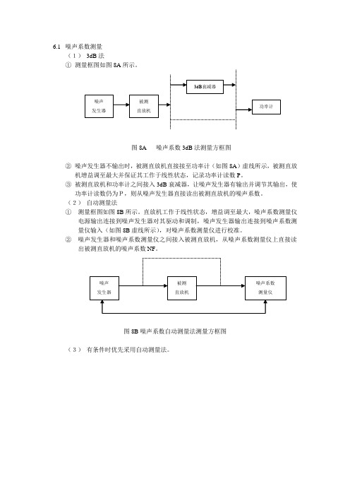
(1) 3dB 法
① 测量框图如图8A 所示。
图8A 噪声系数3dB 法测量方框图
② 噪声发生器不输出时,被测直放机直接接至功率计(如图8A )虚线所示,被测直放
机增益调至最大并保证其工作于线性状态,记录功率计读数P 。
③ 被测直放机和功率计之间接入3dB 衰减器,让噪声发生器有输出并调节其输出,使
功率计读数仍为P,则从噪声发生器直接读出被测直放机的噪声系数。
(2) 自动测量法
① 测量框图如图8B 所示。
直放机工作于线性状态,增益调至最大,噪声系数测量仪
电源输出连接到噪声发生器对其驱动和调制,噪声发生器输出连接到噪声系数测量仪输入(如图8B 虚线所示),对噪声系数测量仪进行校准。
② 噪声发生器和噪声系数测量仪之间接入被测直放机,从噪声系数测量仪上直接读
出被测直放机的噪声系数NF 。
图8B 噪声系数自动测量法测量方框图
(3) 有条件时优先采用自动测量法。
噪声 发生器 被测 直放机 功率计 3dB 衰减器 噪声 发生器 噪声系数 测量仪 被测 直放机。
噪声系数测量
Fsys
?
Pgen KT0 B
பைடு நூலகம்GPg ? GN IN ? N ? 2GN IN ? 2N
GPg ? GN IN ? N
F ? GN IN ? N GN IN
F ? GPg ? Pg GN IN N IN
代入
信号源
F ? Pg KT0 B
DUT 功率计
? (ENR ? F ) 1 ? ENR ? 1 FF
Y ? 1 ? ENR F
F ? ENR Y ?1
测出Y,已知ENR就算出噪声系数F。 NF=10LogF。
Y=N2/N1
未加电 : N1=GKT0B+Na
加电: N2=GTHNaKB+N a
N2=YN1=Y(GKT0B+Na)
GTHKB+N a=Y(GKT0B+Na)
0
ENR/(Y-I)
4.信号发生器测量法
当被测系统噪声系数较大时,可采用信号发生器测量方法。
在被测系统输入端加入负载(环境温度约290K),测量输出噪声
功率P1。然后在输入端加入信号发生器,使信号发生器输出频率在
测量范围内。调整信号发生器输出功率,使被测系统输出功率P2比
P1高3dB。可得出噪声系数:
测试结果
频谱分 析仪
-50dBm -70dBm
RBW=100KHz
噪声密度PND=-70dBm-10Log(100000Hz)=-120dBm 计算结果:NF=-120dBm+174-(-50dBm-(-100dBm)=4dB
(3) Y因子法
图 5-5Y 因子法测试噪声系数
超噪比 : ENR ? TH ? 290 290
微波测量第五章 噪声系数测量
1
噪声系数测试
第一节 基本概念 第二节 手动测量 两倍功率方法噪声系数测量 Y因子法噪声系数测量 第三节 自动噪声系数测量 第四节 影响噪声系数测试精度的一些因素 补充内容: 级联电路的噪声系数计算
2
第一节 基本概念
噪声特性是元件和系统的最重要参数之 一,是元件和系统性能水平的重要体现. 为了更好的理解噪声的重要性,我们首先 举一个较形象了例子:在海边用望远镜观察 海上的船只.
29
14
Y因子法噪声系数测量方框图
15
第三节 自动噪声系数测量
自动噪声系数测量需要用噪声源和自动噪 声测试仪完成
16
17
18
例:放大器 测试
19
例:变频器 测试
20
第四节 影响噪声系数测试精度的一些因素
21
22
环境温度: 获得外部噪声的值,标准的温度(T0)被设 定为290K,制造商所给出的超噪比与它相关, 所以,温度的变化会导致噪声系数测量误差
11
4.2.1两倍功率方法噪声系数测量
主要思想: 根据噪声系数计算公式,如果N2=2N1,则 方程变为NF= ENR.
12
两倍功率方法噪声系数测量方框图
13
4.2.2 Y因子法噪声系数测量
设Y= N2/ N1, 则有NF= = ENR- 10lg (Y-1) 从方程可以看出,不需要测出N2和N1的绝 对值,而只需测出他们比值即Y,就可以确定 NF,这就是这个方法名称的原因.
9
另外,噪声温度也可以用于表述器件或系统 的噪声性能,下面的公式表述了噪声系数与 噪声温度的关系: NF=10lg (1+TN/290) TN即称为噪声温度,单位是K.
(优选)噪声系数测试课件
信号发生器测量法
当被测噪声系数较大时,采用这种方法.
在被测系统输入端加入负载(环境温度约为290K),测量输出 噪声功率P1。然后在输入端接上信号发生器,使信号输出频率 在测量频带范围内。调整信号发生器的输出功率,使被测系统 输出功率P2比P1高3dB。可得噪声系数:
Fsys=Pgen/KT0B 上式中Pgen是信号发生器的输出功率。
(优选)噪声系数测试课件
噪声电压
电阻产生噪声的标准方程
e2 4kTBR
k是波尔兹曼常数 T是绝对温度 B是带宽(Hz) R是电阻( )
Te:等效噪声温度
N1、N2分别表示待测网络接标准 噪声源
超噪比ENR(Excess Noise Ratio)
• ENR不确定度; • 环境温度的影响 • 噪声信号测试线性度 • 被测件工作线性 • 外部干扰信号 • 失配误差
• ……
式中
修正项
10lg[1 Y (Tc T0 ) ] Th T0
当Tc等于标准温度T0时,修正项为零,因此
F(dB) ENR(dB) 10lg(Y 1)
噪声系数线性表达为
Fsys=ENR/(Y-1)
当噪声系数>>ENR时,Y接近于1,此时 测量精度降低。通常噪声系数比ENR大10dB 时,Y- 参数测量法会带来较大的误差.
噪声源超过标准噪声温度T0热噪声的倍数。 即
ENR T T0
或
T0
ENR(dB) 10 lg T T0 T0
噪声系数计算
Y系数方程
(Th 1) Y (Tc 1)
F T0
T0
Y 1
ENR [1 Y (Tc T0 ) ]
Y 1
Th T0
噪声系数计算
噪声系数的含义和测量方法
噪声系数的含义和测量方法
噪声系数是指信号的输入与输出之间的不匹配程度。
它描述了信号传
输中由于不同因素引入的噪声与理论信号的误差比例。
噪声系数越低,表
示信号传输的质量越好。
测量噪声系数的方法主要有两种:器件法和级联法。
1.器件法:这种方法通过对测试样品进行直接测试来测量噪声系数。
测试过程中,利用馈电器件法将器件与参考元件相比较。
参考元件是已知
噪声性能的稳定器件,通常是一种电阻。
通过将被测器件和参考电阻器件
进行比较,可以计算出被测器件的噪声系数。
测量噪声系数时需要注意以下几点:
1.测试环境的干扰要尽可能减少,如尽量避免有其他电磁干扰源的存在。
2.测试过程中需要采用高灵敏度的仪器和设备进行测量,以保证准确性。
3.测量结果可能受到温度、频率等因素的影响,需要进行相应的修正。
4.测量时需要注意信号与噪声的区分,以避免噪声信号被错误地计入
信号中。
噪声系数的大小与信号传输过程中的损耗和噪声有关。
信号传输过程
中会受到各种因素的影响,如电阻、电感、电容、温度等。
这些因素会引
入噪声,导致信号损失和畸变。
噪声系数表示噪声引入的程度,即信号损
失与噪声之间的比值。
测量噪声系数的目的是为了评估信号传输的质量,找出信号传输过程
中引入的噪声和损耗。
这样可以针对噪声源采取相应的优化和改善措施,
提高信号传输系统的性能。
对于需要高质量信号的应用领域,如通信系统、射频系统等,噪声系数的测量和优化具有重要的意义。
- 1、下载文档前请自行甄别文档内容的完整性,平台不提供额外的编辑、内容补充、找答案等附加服务。
- 2、"仅部分预览"的文档,不可在线预览部分如存在完整性等问题,可反馈申请退款(可完整预览的文档不适用该条件!)。
- 3、如文档侵犯您的权益,请联系客服反馈,我们会尽快为您处理(人工客服工作时间:9:00-18:30)。
4.2.1两倍功率方法噪声系数测量
主要思想: 根据噪声系数计算公式,如果N2=2N1,则 方程变为NF= ENR.
12
两倍功率方法噪声系数测量方框图
13
4.2.2 Y因子法噪声系数测量
设Y= N2/ N1, 则有NF= = ENR- 10lg (Y-1) 从方程可以看出,不需要测出N2和N1的绝 对值,而只需测出他们比值即Y,就可以确定 NF,这就是这个方法名称的原因.
3
4
5
6
7
定义: 噪声即元件或系统内部产生的干扰,从 而导致电路的性能恶化. 最噪声的量化主要有两个参数,他们是相关 的,一个是噪声因子,第二个是噪声系数.
8
噪声因子的定义是输入信噪比与输出信噪 比的比值,即 F= (Si/Ni) / (So/No) 噪声系数是噪声因子的对数,即: NF=10lg F 噪声系数的单位是dB,实际应用中通常采用 噪声系数.
9
另外,噪声温度也可以用于表述器件或系统 的噪声性能,下面的公式表述了噪声系数与 噪声温度的关系: NF=10lg (1+TN/290) TN即称为噪声温度,单位是K. 要熟悉 F, NF 和 TN之间的关系
10
第二节 手动测量
噪声系数的计算公式如下 NF=10lg (T2-T0)/T0 -10lg (N2/ N1-1) = ENR- 10lg (N2/ N1-1) 式中: ENR= 10lg (T2-T0)/T0 是超噪比:其含义 是噪声源超过标准噪声温度T0热噪声的倍 数. ENR一般由噪声发生器技术说明书给出. N2: 当噪声源开启时的噪声功率 N1: 当噪声源关闭时的噪声功率
第四章 噪声系数测试
1
噪声系数测试
第一节 基本概念 第二节 手动测量 两倍功率方法噪声系数测量 Y因子法噪声系数测量 第三节 自动噪声系数测量 第四节 影响噪声系数测试精度的一些因素 补充内容: 级联电路的噪声系数计算
2
第一节 基本概念
噪声特性是元件和系统的最重要参数之 一,是元件和系统性能水平的重要体现. 为了更好的理解噪声的重要性,我们首先 举一个较形象了例子:在海边用24
25
噪声系数仪的不确定度 自动噪声系数测量当中所用的噪声系数仪 组成部件比较多,所以它的不确定性的影响 因素也比较多,平方率检波的改变,老化影响 等. 电缆损耗 外部噪声源与DUT间被引入任何损耗都会 影响DUT的噪声系数测试精度.
26
补充内容: 级联电路的噪声系数计算
27
28
29
14
Y因子法噪声系数测量方框图
15
第三节 自动噪声系数测量
自动噪声系数测量需要用噪声源和自动噪 声测试仪完成
16
17
18
例:放大器 测试
19
例:变频器 测试
20
第四节 影响噪声系数测试精度的一些因素
21
22
环境温度: 获得外部噪声的值,标准的温度(T0)被设 定为290K,制造商所给出的超噪比与它相关, 所以,温度的变化会导致噪声系数测量误差