贝叶斯正则化Bayesian BP Regulation
LM 优化算法和贝叶斯正则化算法
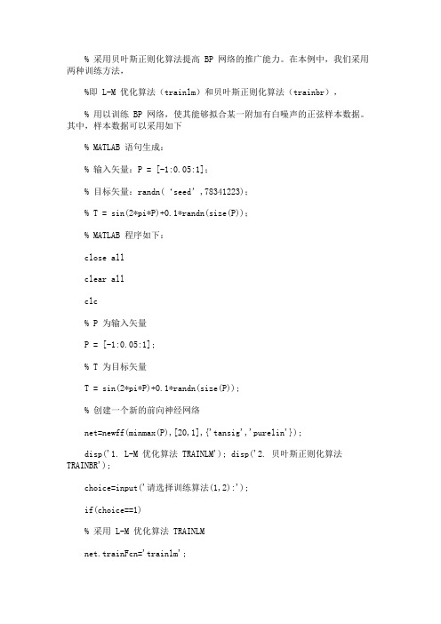
% 采用贝叶斯正则化算法提高 BP 网络的推广能力。
在本例中,我们采用两种训练方法,%即 L-M 优化算法(trainlm)和贝叶斯正则化算法(trainbr),% 用以训练 BP 网络,使其能够拟合某一附加有白噪声的正弦样本数据。
其中,样本数据可以采用如下% MATLAB 语句生成:% 输入矢量:P = [-1:0.05:1];% 目标矢量:randn(‘seed’,78341223);% T = sin(2*pi*P)+0.1*randn(size(P));% MATLAB 程序如下:close allclear allclc% P 为输入矢量P = [-1:0.05:1];% T 为目标矢量T = sin(2*pi*P)+0.1*randn(size(P));% 创建一个新的前向神经网络net=newff(minmax(P),[20,1],{'tansig','purelin'});disp('1. L-M 优化算法 TRAINLM'); disp('2. 贝叶斯正则化算法TRAINBR');choice=input('请选择训练算法(1,2):');if(choice==1)% 采用 L-M 优化算法 TRAINLMnet.trainFcn='trainlm';% 设置训练参数net.trainParam.epochs = 500; net.trainParam.goal = 1e-6;% 重新初始化net=init(net);pause;elseif(choice==2)% 采用贝叶斯正则化算法 TRAINBR net.trainFcn='trainbr';% 设置训练参数net.trainParam.epochs = 500; % 重新初始化net = init(net);pause;开放教育试点汉语言文学专业毕业论文浅谈李白的诗文风格姓名:李小超学号:20097410060058学校:焦作电大指导教师:闫士有浅谈李白的诗文风格摘要:李白的浪漫主义诗风是艺术表现的最高典范,他把艺术家自身的人格精神与作品的气象、意境完美结合,浑然一体,洋溢着永不衰竭和至高无上的创造力。
机器学习算法调参技巧解读

机器学习算法调参技巧解读机器学习算法调参是提高预测模型性能的重要一环。
在实际应用中,不同的数据集和问题需要采用不同的算法和参数配置,因此,理解和掌握机器学习算法调参的技巧对于算法工程师和数据科学家来说是至关重要的。
本文将深入解读机器学习算法调参的技巧和方法。
一、算法调参的意义和目标在机器学习中,调参是指选择合适的参数或参数组合,以优化模型在训练集和测试集上的性能。
一般来说,调参的目标是找到最佳参数组合,使得模型具有较高的准确性、泛化能力和稳定性。
二、常见的算法调参方法1. 网格搜索(Grid Search)网格搜索是一种常用的调参方法,它通过系统地遍历参数空间中的每一种可能组合,从而寻找最佳的参数组合。
网格搜索的思想简单直观,但是对于参数空间较大的情况下会效率较低。
2. 随机搜索(Random Search)随机搜索与网格搜索相比,它在参数空间中随机采样一组参数,不同于网格搜索的是,随机搜索是基于随机选择,因此可以避免网格搜索的缺点。
相对于网格搜索,随机搜索的优势在于它对参数空间的探索更加灵活。
3. 贝叶斯优化(Bayesian Optimization)贝叶斯优化是一种基于贝叶斯推断的调参方法。
它通过利用历史观察样本的性能,动态地调整参数搜索空间,以便更好地探索参数空间。
贝叶斯优化需要根据先验信息初始化,并通过不断收集样本来更新先验信息,从而找到最佳的参数组合。
4. 集成学习(Ensemble Methods)集成学习是指通过组合多个预测模型来提高模型的整体性能。
在参数调优中,我们可以通过集成学习的方法,如随机森林、梯度提升决策树等,结合不同参数配置的模型,来获得更好的模型表现。
三、参数的选择和调节在进行算法调参时,需要重点关注以下几个方面的参数:1. 学习率(Learning Rate)学习率是指每一轮迭代中参数更新的步长。
较小的学习率可以使模型更加稳定,但训练时间会变长;较大的学习率可以加速模型的学习速度,但可能会导致模型不稳定。
机器学习算法的参数调优方法

机器学习算法的参数调优方法机器学习算法的参数调优是提高模型性能和泛化能力的关键步骤。
在机器学习过程中,正确选择和调整算法的参数可以显著影响模型的预测准确性和鲁棒性。
本文将介绍一些常见的机器学习算法的参数调优方法,以帮助您优化您的模型。
1. 网格搜索(Grid Search)网格搜索是最常用和直观的参数调优方法之一。
它通过穷举地尝试所有可能的参数组合,找到在给定评价指标下最好的参数组合。
具体而言,网格搜索将定义一个参数网格,其中包含要调整的每个参数及其可能的取值。
然后,通过遍历参数网格中的所有参数组合,评估每个组合的性能,并选择具有最佳性能的参数组合。
网格搜索的优点是简单易用,并且能够覆盖所有可能的参数组合。
然而,由于穷举搜索的复杂性,当参数的数量较多或参数取值范围较大时,网格搜索的计算代价将变得非常高。
2. 随机搜索(Random Search)随机搜索是一种更高效的参数调优方法。
与网格搜索不同,随机搜索不需要遍历所有可能的参数组合,而是通过在参数空间内随机选择参数组合来进行评估。
这种方法更适用于参数空间较大的情况,因为它可以更快地对参数进行搜索和评估。
随机搜索的主要优势是它可以更高效地搜索参数空间,特别是在目标参数与性能之间没有明确的关系时。
然而,随机搜索可能无法找到全局最佳参数组合,因为它没有对参数空间进行全面覆盖。
3. 贝叶斯优化(Bayesian Optimization)贝叶斯优化是一种通过构建模型来优化目标函数的参数调优方法。
它通过根据已经评估过的参数组合的结果来更新对目标函数的概率模型。
然后,通过在参数空间中选择具有高期望改进的参数组合来进行评估。
这种方法有效地利用了先前观察到的信息,并且可以在相对较少的试验次数中找到最佳参数组合。
贝叶斯优化的优点是可以自适应地根据先前的观察结果进行参数选择,并在较少的试验次数中达到较好的性能。
然而,贝叶斯优化的计算代价较高,并且对于大规模数据集可能会面临挑战。
贝叶斯正则化的BP神经网络在经济预测中的应用

贝叶斯正则化的B P神经网络在经济预测中的应用
华中师范大学数学与统计学学院 李旭军
[摘 要]本文应用Bayesian正则化算法改进BP神经网络泛化能力。
通过对湖北省1985年—2004年关于经济发展水
平的数据进行拟和以及预测,结果表明采用Bayesian正则化算法比相同条件下采用其他改进算法泛化能力要好,收
敛速度快、预测精度高,方法简单,操作方便。
实例分析表明,贝叶斯正则化算法优化BP神经网络的方法是令人满意的,对经济预测有良好的预测效果。
[关键词]BP神经网络 贝叶斯正则 经济预测
—
—
7
6
—
86—
—96—。
贝叶斯正则化算法

贝叶斯正则化算法贝叶斯正则化算法是一种基于贝叶斯概率框架的机器学习算法,它是建立在贝叶斯概率模型的基础上的一种统计学习方法。
它将传统的机器学习方法(如线性回归和支持向量机)与贝叶斯理论相结合,将贝叶斯概率模型用于机器学习,从而提高机器学习的准确性和效率。
本文将回顾贝叶斯正则化算法的基本原理和优点,以及它如何用于机器学习。
一、基本原理贝叶斯正则化算法是一种基于贝叶斯概率模型的机器学习算法。
贝叶斯概率模型假设数据生成过程可以用概率分布来描述,并通过贝叶斯公式来推断数据的潜在模式。
在贝叶斯正则化算法中,模型参数的估计值是通过最大后验概率(MAP)确定的,即目标函数是参数的函数的最大后验概率。
贝叶斯正则化算法的核心思想是,未知参数的估计值应该是参数的概率分布的最大值。
在贝叶斯正则化中,参数的概率分布是一个拉普拉斯先验分布,它是一个较简单的分布,可以用来描述参数的未知性,从而降低机器学习模型的过拟合。
二、优点贝叶斯正则化算法具有许多优点,其中最重要的优点是它可以显著改善机器学习模型的准确性和效率。
此外,贝叶斯正则化算法还可以增加模型的稳定性和可解释性。
首先,贝叶斯正则化算法可以显著提高机器学习模型的准确性。
贝叶斯正则化算法将传统的机器学习方法(如线性回归和支持向量机)与贝叶斯理论相结合,可以更好地拟合数据,从而提高机器学习模型的准确性。
此外,贝叶斯正则化算法还可以提高机器学习模型的效率。
它通过拉普拉斯先验分布将参数的不确定性考虑在内,从而降低对数据量的要求,从而提高机器学习模型的效率。
另外,贝叶斯正则化算法还可以提高模型的稳定性。
传统的机器学习模型往往会受到较大的噪声影响,而贝叶斯正则化算法可以有效减少噪声对模型的影响,从而提高模型的稳定性。
最后,贝叶斯正则化算法还可以增强模型的可解释性。
贝叶斯正则化算法可以将模型参数的不确定性表达出来,从而使模型更容易解释。
三、应用贝叶斯正则化算法可以用于多种机器学习应用,如线性回归、支持向量机和神经网络等。
贝叶斯准则

判决式为:
q ( z ) p H0
2.派生贝叶斯准则及计算 例2:考虑二元假设, H0: z=n H1: z=A+n 其中n~N(0, n ),先验概率p=q=0.5且A>0,试根据一次观测数
2
据z,给出最小总错误概率准则判决表达式及错误概率。
2.派生贝叶斯准则及计算 解:
2.派生贝叶斯准则及计算 1、最小总错误概率准则(MPE)
在通信系统中,通常假定
பைடு நூலகம்
c00 c11 0, c01 c10 1 ,即正确的
判决不付出代价,错误判决代价相同。
C C00 Pc C10 q C01 C11PD p q p Pe
f ( z)
z
Z1
Z1 Z1
1.贝叶斯准则及计算
C10 C00 q p( z | H1 ) p( z | H 0 ) 0 C01 C11 p
p ( z | H1 ) 似然比: ( z ) p( z | H 0 )
H1
门限:
(C10 C00 )q (C01 C11 ) p
C10 C00 q C C01 C11 p
C10 C00 q C 1 p( z | H1 ) p( z | H 0 ) dz Z1 C01 C11 p
1.贝叶斯准则及计算
C10 C00 q f ( z ) p( z | H1 ) p( z | H 0 ) C01 C11 p
1.贝叶斯准则及计算 解 : ( 1)
1 p( z | H 0 ) exp ( z 1)2
参数模型估计算法

参数模型估计算法参数模型估计算法是指根据已知的数据样本,通过其中一种数学模型来估计模型中的参数值。
这些参数值用于描述模型中的各种特征,例如均值、方差、回归系数等。
参数模型估计算法在统计学和机器学习等领域中有着广泛的应用,可以用来解决预测、分类、回归等问题。
常见的参数模型估计算法包括最小二乘法、最大似然估计和贝叶斯估计等。
下面将逐一介绍这些算法的原理和实现方法。
1. 最小二乘法(Least Squares Method):最小二乘法是一种常见的参数估计方法,用于拟合线性回归模型。
其思想是选择模型参数使得观测数据与预测值之间的差平方和最小。
通过最小化误差函数,可以得到方程的最优解。
最小二乘法适用于数据符合线性关系的情况,例如回归分析。
2. 最大似然估计(Maximum Likelihood Estimation):最大似然估计是一种常见的参数估计方法,用于估计模型参数使得给定观测数据的概率最大。
其基本思想是找到一组参数值,使得给定数据产生的可能性最大化。
最大似然估计适用于数据符合其中一种概率分布的情况,例如正态分布、泊松分布等。
3. 贝叶斯估计(Bayesian Estimation):贝叶斯估计是一种基于贝叶斯定理的参数估计方法,用于估计模型参数的后验分布。
其思想是先假设参数的先验分布,然后根据观测数据来更新参数的后验分布。
贝叶斯估计能够将先验知识和数据信息相结合,更加准确地估计模型参数。
除了以上提到的算法,还有一些其他的参数模型估计算法,例如最小二乘支持向量机(LSSVM)、正则化方法(如岭回归和LASSO)、逻辑回归等。
这些算法在不同的情境下具有不同的应用。
例如,LSSVM适用于非线性分类和回归问题,正则化方法用于解决高维数据的过拟合问题,逻辑回归用于二分类问题。
无论是哪种参数模型估计算法,都需要预先定义一个合适的模型以及其参数空间。
然后,通过选择合适的损失函数或优化目标,采用数值优化或迭代方法求解模型参数的最优解。
调参的方法

调参的方法机器学习领域中,调参是非常重要的一个环节。
调参的目的是找到最优的超参数组合,以提高模型的性能和泛化能力。
本文将介绍10个关于调参的方法及其详细描述,帮助读者更好地理解和掌握调参技巧。
1. 网格搜索(Grid Search)网格搜索是一种穷举搜索的方法,它会遍历超参数空间中的所有可能组合,以找到最佳组合。
网格搜索的缺点是计算时间可能比较长,但它可以找到全局最优的超参数组合。
2. 随机搜索(Random Search)与网格搜索不同的是,随机搜索不会遍历超参数空间中的所有可能组合,而是在随机的超参数组合中选择。
随机搜索具有时间效率高的优点,但可能不太能保证找到全局最优的超参数组合。
3. 贝叶斯优化(Bayesian Optimization)贝叶斯优化是一种基于贝叶斯定理和高斯过程回归的方法。
它会根据之前的尝试结果和模型预测来选择下一个超参数组合。
贝叶斯优化对超参数空间的搜索策略更加智能化,可以大大提高调参效率。
4. 学习曲线(Learning Curve)学习曲线是一种可视化方法,它会绘制不同超参数组合下训练集和测试集的准确率(或其他性能指标)与训练数据量之间的关系。
通过学习曲线,我们可以判断模型是否处于欠拟合或过拟合状态,以及确定最佳超参数组合。
5. 验证曲线(Validation Curve)验证曲线与学习曲线类似,它会绘制某一个超参数的不同取值下的训练集和测试集准确率(或其他性能指标)与超参数取值之间的关系。
通过验证曲线,我们可以确定某个超参数的最佳取值范围。
6. 交叉验证(Cross-Validation)交叉验证是一种将数据集划分为多个子集的方法。
在每一次交叉验证中,其中一个子集被作为测试集,其余子集则被作为训练集。
通过交叉验证,我们可以减小因数据划分不合理造成的误差,从而更好地评估模型性能和泛化能力。
7. 正则化(Regularization)正则化是一种限制模型复杂度的方法。
- 1、下载文档前请自行甄别文档内容的完整性,平台不提供额外的编辑、内容补充、找答案等附加服务。
- 2、"仅部分预览"的文档,不可在线预览部分如存在完整性等问题,可反馈申请退款(可完整预览的文档不适用该条件!)。
- 3、如文档侵犯您的权益,请联系客服反馈,我们会尽快为您处理(人工客服工作时间:9:00-18:30)。
APPLICATION OF BAYESIAN REGULARIZED BP NEURALNETWORK MODEL FOR TREND ANALYSIS,ACIDITY ANDCHEMICAL COMPOSITION OF PRECIPITATION IN NORTHCAROLINAMIN XU1,GUANGMING ZENG1,2,∗,XINYI XU1,GUOHE HUANG1,2,RU JIANG1and WEI SUN21College of Environmental Science and Engineering,Hunan University,Changsha410082,China;2Sino-Canadian Center of Energy and Environment Research,University of Regina,Regina,SK,S4S0A2,Canada(∗author for correspondence,e-mail:zgming@,ykxumin@,Tel.:86–731-882-2754,Fax:86-731-882-3701)(Received1August2005;accepted12December2005)Abstract.Bayesian regularized back-propagation neural network(BRBPNN)was developed for trend analysis,acidity and chemical composition of precipitation in North Carolina using precipitation chemistry data in NADP.This study included two BRBPNN application problems:(i)the relationship between precipitation acidity(pH)and other ions(NH+4,NO−3,SO2−4,Ca2+,Mg2+,K+,Cl−and Na+) was performed by BRBPNN and the achieved optimal network structure was8-15-1.Then the relative importance index,obtained through the sum of square weights between each input neuron and the hidden layer of BRBPNN(8-15-1),indicated that the ions’contribution to the acidity declined in the order of NH+4>SO2−4>NO−3;and(ii)investigations were also carried out using BRBPNN with respect to temporal variation of monthly mean NH+4,SO2−4and NO3−concentrations and their optimal architectures for the1990–2003data were4-6-1,4-6-1and4-4-1,respectively.All the estimated results of the optimal BRBPNNs showed that the relationship between the acidity and other ions or that between NH+4,SO2−4,NO−3concentrations with regard to precipitation amount and time variable was obviously nonlinear,since in contrast to multiple linear regression(MLR),BRBPNN was clearly better with less error in prediction and of higher correlation coefficients.Meanwhile,results also exhibited that BRBPNN was of automated regularization parameter selection capability and may ensure the excellentfitting and robustness.Thus,this study laid the foundation for the application of BRBPNN in the analysis of acid precipitation.Keywords:Bayesian regularized back-propagation neural network(BRBPNN),precipitation,chem-ical composition,temporal trend,the sum of square weights1.IntroductionCharacterization of the chemical nature of precipitation is currently under con-siderable investigations due to the increasing concern about man’s atmospheric inputs of substances and their effects on land,surface waters,vegetation and mate-rials.Particularly,temporal trend and chemical composition has been the subject of extensive research in North America,Canada and Japan in the past30years(Zeng Water,Air,and Soil Pollution(2006)172:167–184DOI:10.1007/s11270-005-9068-8C Springer2006168MIN XU ET AL.and Flopke,1989;Khawaja and Husain,1990;Lim et al.,1991;Sinya et al.,2002; Grimm and Lynch,2005).Linear regression(LR)methods such as multiple linear regression(MLR)have been widely used to develop the model of temporal trend and chemical composition analysis in precipitation(Sinya et al.,2002;George,2003;Aherne and Farrell,2002; Christopher et al.,2005;Migliavacca et al.,2004;Yasushi et al.,2001).However, LR is an“ill-posed”problem in statistics and sometimes results in the instability of the models when trained with noisy data,besides the requirement of subjective decisions to be made on the part of the investigator as to the likely functional (e.g.nonlinear)relationships among variables(Burden and Winkler,1999;2000). On the other hand,recently,there has been increasing interest in estimating the uncertainties and nonlinearities associated with impact prediction of atmospheric deposition(Page et al.,2004).Besides precipitation amount,human activities,such as local and regional land cover and emission sources,the actual role each plays in determining the concentration at a given location is unknown and uncertain(Grimm and Lynch,2005).Therefore,it is of much significance that the model of temporal variation and precipitation chemistry is efficient,gives unambiguous models and doesn’t depend upon any subjective decisions about the relationships among ionic concentrations.In this study,we propose a Bayesian regularized back-propagation neural net-work(BRBPNN)to overcome MLR’s deficiencies and investigate nonlinearity and uncertainty in acid precipitation.The network is trained through Bayesian reg-ularized methods,a mathematical process which converts the regression into a well-behaved,“well-posed”problem.In contrast to MLR and traditional neural networks(NNs),BRBPNN has more performance when the relationship between variables is nonlinear(Sovan et al.,1996;Archontoula et al.,2003)and more ex-cellent generalizations because BRBPNN is of automated regularization parameter selection capability to obtain the optimal network architecture of posterior distri-bution and avoid over-fitting problem(Burden and Winkler,1999;2000).Thus,the main purpose of our paper is to apply BRBPNN method to modeling the nonlinear relationship between the acidity and chemical compositions of precipitation and improve the accuracy of monthly ionic concentration model used to provide pre-cipitation estimates.And both of them are helpful to predict precipitation variables and interpret mechanisms of acid precipitation.2.Theories and Methods2.1.T HEORY OF BAYESIAN REGULARIZED BP NEURAL NETWORK Traditional NN modeling was based on back-propagation that was created by gen-eralizing the Widrow-Hoff learning rule to multiple-layer networks and nonlinear differentiable transfer monly,a BPNN comprises three types ofAPPLICATION OF BAYESIAN REGULARIZED BP NEURAL NETWORK MODEL 169Hidden L ayerInput a 1=tansig(IW 1,1p +b 1 ) Output L ayer a 2=pu relin(LW 2,1a 1+b 2)Figure 1.Structure of the neural network used.R =number of elements in input vector;S =number of hidden neurons;p is a vector of R input elements.The network input to the transfer function tansig is n 1and the sum of the bias b 1.The network output to the transfer function purelin is n 2and the sum of the bias b 2.IW 1,1is input weight matrix and LW 2,1is layer weight matrix.a 1is the output of the hidden layer by tansig transfer function and y (a 2)is the network output.neuron layers:an input layer,one or several hidden layers and an output layer comprising one or several neurons.In most cases only one hidden layer is used (Figure 1)to limit the calculation time.Although BPNNs with biases,a sigmoid layer and a linear output layer are capable of approximating any function with a finite number of discontinuities (The MathWorks,),we se-lect tansig and pureline transfer functions of MATLAB to improve the efficiency (Burden and Winkler,1999;2000).Bayesian methods are the optimal methods for solving learning problems of neural network,which can automatically select the regularization parameters and integrates the properties of high convergent rate of traditional BPNN and prior information of Bayesian statistics (Burden and Winkler,1999;2000;Jouko and Aki,2001;Sun et al.,2005).To improve generalization ability of the network,the regularized training objective function F is denoted as:F =αE w +βE D (1)where E W is the sum of squared network weights,E D is the sum of squared net-work errors,αand βare objective function parameters (regularization parameters).Setting the correct values for the objective parameters is the main problem with im-plementing regularization and their relative size dictates the emphasis for training.Specially,in this study,the mean square errors (MSE)are chosen as a measure of the network training approximation.Set a desired neural network with a training data set D ={(p 1,t 1),(p 2,t 2),···,(p i ,t i ),···,(p n ,t n )},where p i is an input to the network,and t i is the corresponding target output.As each input is applied to the network,the network output is compared to the target.And the error is calculated as the difference between the target output and the network output.Then170MIN XU ET AL.we want to minimize the average of the sum of these errors(namely,MSE)through the iterative network training.MSE=1nni=1e(i)2=1nni=1(t(i)−a(i))2(2)where n is the number of sample set,e(i)is the error and a(i)is the network output.In the Bayesian framework the weights of the network are considered random variables and the posterior distribution of the weights can be updated according to Bayes’rule:P(w|D,α,β,M)=P(D|w,β,M)P(w|α,M)P(D|α,β,M)(3)where M is the particular neural network model used and w is the vector of net-work weights.P(w|α,M)is the prior density,which represents our knowledge of the weights before any data are collected.P(D|w,β,M)is the likelihood func-tion,which is the probability of the data occurring,given that the weights w. P(D|α,β,M)is a normalization factor,which guarantees that the total probability is1.Thus,we havePosterior=Likelihood×PriorEvidence(4)Likelyhood:A network with a specified architecture M and w can be viewed as making predictions about the target output as a function of input data in accordance with the probability distribution:P(D|w,β,M)=exp(−βE D)Z D(β)(5)where Z D(β)is the normalization factor:Z D(β)=(π/β)n/2(6) Prior:A prior probability is assigned to alternative network connection strengths w,written in the form:P(w|α,M)=exp(−αE w)Z w(α)(7)where Z w(α)is the normalization factor:Z w(α)=(π/α)K/2(8)APPLICATION OF BAYESIAN REGULARIZED BP NEURAL NETWORK MODEL171 Finally,the posterior probability of the network connections w is:P(w|D,α,β,M)=exp(−(αE w+βE D))Z F(α,β)=exp(−F(w))Z F(α,β)(9)Setting regularization parametersαandβ.The regularization parameters αandβdetermine the complexity of the model M.Now we apply Bayes’rule to optimize the objective function parametersαandβ.Here,we haveP(α,β|D,M)=P(D|α,β,M)P(α,β|M)P(D|M)(10)If we assume a uniform prior density P(α,β|M)for the regularization parame-tersαandβ,then maximizing the posterior is achieved by maximizing the likelihood function P(D|α,β,M).We also notice that the likelihood function P(D|α,β,M) on the right side of Equation(10)is the normalization factor for Equation(3). According to Foresee and Hagan(1997),we have:P(D|α,β,M)=P(D|w,β,M)P(w|α,M)P(w|D,α,β,M)=Z F(α,β)Z w(α)Z D(β)(11)In Equation(11),the only unknown part is Z F(α,β).Since the objective function has the shape of a quadratic in a small area surrounding the minimum point,we can expand F(w)around the minimum point of the posterior density w MP,where the gradient is zero.Solving for the normalizing constant yields:Z F(α,β)=(2π)K/2det−1/2(H)exp(−F(w MP))(12) where H is the Hessian matrix of the objective function.H=β∇2E D+α∇2E w(13) Substituting Equation(12)into Equation(11),we canfind the optimal values for αandβ,at the minimum point by taking the derivative with respect to each of the log of Equation(11)and set them equal to zero,we have:αMP=γ2E w(w MP)andβMP=n−γ2E D(w MP)(14)whereγ=K−αMP trace−1(H MP)is the number of effective parameters;n is the number of sample set and K is the total number of parameters in the network. The number of effective parameters is a measure of how many parameters in the network are effectively used in reducing the error function.It can range from zero to K.After training,we need to do the following checks:(i)Ifγis very close to172MIN XU ET AL.K,the network may be not large enough to properly represent the true function.In this case,we simply add more hidden neurons and retrain the network to make a larger network.If the larger network has the samefinalγ,then the smaller network was large enough;and(ii)if the network is sufficiently large,then a second larger network will achieve comparable values forγ.The Bayesian optimization of the regularization parameters requires the com-putation of the Hessian matrix of the objective function F(w)at the minimum point w MP.To overcome this problem,the Gauss-Newton approximation to Hessian ma-trix has been proposed by Foresee and Hagan(1997).Here are the steps required for Bayesian optimization of the regularization parameters:(i)Initializeα,βand the weights.After thefirst training step,the objective function parameters will recover from the initial setting;(ii)Take one step of the Levenberg-Marquardt algorithm to minimize the objective function F(w);(iii)Computeγusing the Gauss-Newton approximation to Hessian matrix in the Levenberg-Marquardt training algorithm; (iv)Compute new estimates for the objective function parametersαandβ;And(v) now iterate steps ii through iv until convergence.2.2.W EIGHT CALCULATION OF THE NETWORKGenerally,one of the difficult research topics of BRBPNN model is how to obtain effective information from a neural network.To a certain extent,the network weight and bias can reflect the complex nonlinear relationships between input variables and output variable.When the output layer only involves one neuron,the influences of input variables on output variable are directly presented in the influences of input parameters upon the network.Simultaneously,in case of the connection along the paths from the input layer to the hidden layer and along the paths from the hidden layer to the output layer,it is attempted to study how input variables react to the hidden layer,which can be considered as the impacts of input variables on output variable.According to Joseph et al.(2003),the relative importance of individual input variable upon output variable can be expressed as:I=Sj=1ABS(w ji)Numi=1Sj=1ABS(w ji)(15)where w ji is the connection weight from i input neuron to j hidden neuron,ABS is an absolute function,Num,S are the number of input variables and hidden neurons, respectively.2.3.M ULTIPLE LINEAR REGRESSIONThis study attempts to ascertain whether BRBPNN are preferred to MLR models widely used in the past for temporal variation of acid precipitation(Buishand et al.,APPLICATION OF BAYESIAN REGULARIZED BP NEURAL NETWORK MODEL173 1988;Dana and Easter,1987;MAP3S/RAINE,1982).MLR employs the following regression model:Y i=a0+a cos(2πi/12−φ)+bi+cP i+e i i=1,2,...12N(16) where N represents the number of years in the time series.In this case,Y i is the natural logarithm of the monthly mean concentration(mg/L)in precipitation for the i th month.The term a0represents the intercept.P i represents the natural logarithm of the precipitation amount(ml)for the i th month.The term bi,where i(month) goes from1to12N,represents the monotonic trend in concentration in precipitation over time.To facilitate the estimation of the coefficients a0,a,b,c andφfollowing Buishand et al.(1988)and John et al.(2000),the reparameterized MLR model was established and thefinal form of Equation(16)becomes:Y i=a0+αcos(2πi/12)+βsin(2πi/12)+bi+cP i+e i i=1,2,...12N(17)whereα=a cosϕandβ=a sinϕ.a0,α,β,b and c of the regression coefficients in Equation(17)are estimated using ordinary least squares method.2.4.D ATA SET SELECTIONPrecipitation chemistry data used are derived from NADP(the National At-mospheric Deposition Program),a nationwide precipitation collection network founded in1978.Monthly precipitation information of nine species(pH,NH+4, NO−3,SO2−4,Ca2+,Mg2+,K+,Cl−and Na+)and precipitation amount in1990–2003are collected in Clinton Crops Research Station(NC35),North Carolina, rmation on the data validation can be found at the NADP website: .The BRBPNN advantages are that they are able to produce models that are robust and well matched to the data.At the end of training,a Bayesian regularized neural network has the optimal generalization qualities and thus there is no need for a test set(MacKay,1992;1995).Husmeier et al.(1999)has also shown theoretically and by example that in a Bayesian regularized neural network,the training and test set performance do not differ significantly.Thus,this study needn’t select the test set and only the training set problem remains.i.Training set of BRBPNN between precipitation acidity and other ions With regard to the relationship between precipitation acidity and other ions,the input neurons are taken from monthly concentrations of NH+4,NO−3,SO2−4,Ca2+, Mg2+,K+,Cl−and Na+.And precipitation acidity(pH)is regarded as the output of the network.174MIN XU ET AL.ii.Training set of BRBPNN for temporal trend analysisBased on the weight calculations of BRBPNN between precipitation acidity and other ions,this study will simulate temporal trend of three main ions using BRBPNN and MLR,respectively.In Equation(17)of MLR,we allow a0,α,β,b and c for the estimated coefficients and i,P i,cos(2πi/12),and sin(2πi/12)for the independent variables.To try to achieve satisfactoryfitting results of BRBPNN model,we similarly employ four unknown items(i,P i,cos(2πi/12),and sin(2πi/12))as the input neurons of BRBPNN,the availability of which will be proved in the following. 2.5.S OFTWARE AND METHODMLR is carried out through SPSS11.0software.BRBPNN is debugged in neural network toolbox of MATLAB6.5for the algorithm described in Section2.1.Concretely,the BRBPNN algorithm is implemented through“trainbr”network training function in MATLAB toolbox,which updates the weight and bias according to Levenberg-Marquardt optimization.The function minimizes both squared errors and weights,provides the number of network parameters being effectively used by the network,and then determines the correct combination so as to produce a network that generalizes well.The training is stopped if the maximum number of epochs is reached,the performance has been minimized to a suitable small goal, or the performance gradient falls below a suitable target.Each of these targets and goals is set at the default values by MATLAB implementation if we don’t want to set them artificially.To eliminate the guesswork required in determining the optimum network size,the training should be carried out many times to ensure convergence.3.Results and Discussions3.1.C ORRELATION COEFfiCIENTS OF PRECIPITATION IONSFrom Table I it shows the correlation coefficients for the ion components and precipitation amount in NC35,which illustrates that the acidity of precipitation results from the integrative interactions of anions and cations and mainly depends upon four species,i.e.SO2−4,NO−3,Ca2+and NH+4.Especially,pH is strongly correlated with SO2−4and NO−3and their correlation coefficients are−0.708and −0.629,respectively.In addition,it can be found that all the ionic species have a negative correlation with precipitation amount,which accords with the theory thatthe higher the precipitation amount,the lower the ionic concentration(Li,1999).3.2.R ELATIONSHIP BETWEEN PH AND CHEMICAL COMPOSITIONS3.2.1.BRBPNN Structure and RobustnessFor the BRBPNN of the relationship between pH and chemical compositions,the number of input neurons is determined based on that of the selected input variables,APPLICATION OF BAYESIAN REGULARIZED BP NEURAL NETWORK MODEL175TABLE ICorrelation coefficients of precipitation ionsPrecipitation Ions Ca2+Mg2+K+Na+NH+4NO−3Cl−SO2−4pH amountCa2+ 1.0000.4620.5480.3490.4490.6270.3490.654−0.342−0.369Mg2+ 1.0000.3810.9800.0510.1320.9800.1230.006−0.303K+ 1.0000.3200.2480.2260.3270.316−0.024−0.237Na+ 1.000−0.0310.0210.9920.0210.074−0.272NH+4 1.0000.7330.0110.610−0.106−0.140NO−3 1.0000.0500.912−0.629−0.258Cl− 1.0000.0490.075−0.265SO2−4 1.000−0.708−0.245pH 1.0000.132 Precipitation 1.000 amountcomprising eight ions of NH+4,NO−3,SO2−4,Ca2+,Mg2+,K+,Cl−and Na+,and the output neuron only includes pH.Generally,the number of hidden neurons for traditional BPNN is roughly estimated through investigating the effects of the repeatedly trained network.But,BRBPNN can automatically search the optimal network parameters in posterior distribution(MacKay,1992;Foresee and Hagan, 1997).Based on the algorithm of Section2.1and Section2.5,the“trainbr”network training function is used to implement BRBPNNs with a tansig hidden layer and a pureline output layer.To acquire the optimal architecture,the BRBPNNs are trained independently20times to eliminate spurious effects caused by the random set of initial weights and the network training is stopped when the maximum number of repetitions reaches3000epochs.Add the number of hidden neurons(S)from1to 20and retrain BRBPNNs until the network performance(the number of effective parameters,MSE,E w and E D,etc.)remains approximately the same.In order to determine the optimal BRBPNN structure,Figure2summarizes the results for training many different networks of the8-S-1architecture for the relationship between pH and chemical constituents of precipitation.It describes MSE and the number of effective parameters changes along with the number of hidden neurons(S).When S is less than15,the number of effective parameters becomes bigger and MSE becomes smaller with the increase of S.But it is noted that when S is larger than15,MSE and the number of effective parameters is roughly constant with any network.This is the minimum number of hidden neurons required to properly represent the true function.From Figure2,the number of hidden neurons (S)can increase until20but MSE and the number of effective parameters are still roughly equal to those in the case of the network with15hidden neurons,which suggests that BRBPNN is robust.Therefore,using BPBRNN technique,we can determine the optimal size8-15-1of neural network.176MIN XU ET AL.Figure2.Changes of optimal BRBPNNs along with the number of hidden neurons.parison of calculations between BRBPNN(8-15-1)and MLR.3.2.2.Prediction Results ComparisonFigure3illustrates the output response of the BRBPNN(8-15-1)with a quite goodfit.Obviously,the calculations of BRBPNN(8-15-1)have much higher correlationcoefficient(R2=0.968)and more concentrated near the isoline than those of MLR. In contrast to the previous relationships between the acidity and other ions by MLR,most of average regression R2achieves less than0.769(Yu et al.,1998;Baez et al.,1997;Li,1999).Additionally,Figures2and3show that any BRBPNN of8-S-1architecture hasbetter approximating qualities.Even if S is equal to1,MSE of BRBPNN(8-1-1)ismuch smaller and superior than that of MLR.Thus,we can judge that there havebeen strong nonlinear relationships between the acidity and other ion concentration,which can’t be explained by MLR,and that it may be quite reasonable to apply aAPPLICATION OF BAYESIAN REGULARIZED BP NEURAL NETWORK MODEL177TABLE IISum of square weights(SSW)and the relative importance(I)from input neurons to hidden layer Ca2+Mg2+K+Na+NH+4NO−3Cl−SO2−4 SSW 2.9589 2.7575 1.74170.880510.4063 4.0828 1.3771 5.2050 I(%)10.069.38 5.92 2.9935.3813.88 4.6817.70neural network methodology to interpret nonlinear mechanisms between the acidity and other input variables.3.2.3.Weight Interpretation for the Acidity of PrecipitationTo interpret the weight of the optimal BRBPNN(8-15-1),Equation(15)is used to evaluate the significance of individual input variable and the calculations are illustrated in Table II.In the eight inputs of BRBPNN(8-15-1),comparatively, NH+4,SO2−4,NO−3,Ca2+and Mg2+have greater impacts upon the network and also indicates thesefive factors are of more significance for the acidity.From Table II it shows that NH+4contributes by far the most(35.38%)to the acidity prediction, while SO2−4and NO−3contribute with17.70%and13.88%,respectively.On the other hand,Ca2+and Mg2+contribute10.06%and9.38%,respectively.3.3.T EMPORAL TREND ANALYSIS3.3.1.Determination of BRBPNN StructureUniversally,there have always been lowfitting results in the analysis of temporal trend estimation in precipitation.For example,the regression R2of NH+4and NO−3 for Vhesapeake Bay Watershed in Grimma and Lynch(2005)are0.3148and0.4940; and the R2of SO2−4,NH+4and NO−3for Japan in Sinya et al.(2002)are0.4205, 0.4323and0.4519,respectively.This study also applies BRBPNN to estimate temporal trend of precipitation chemistry.According to the weight results,we select NH+4,SO2−4and NO−3to predict temporal trends using BRBPNN.Four unknown items(i,P i,cos(2πi/12),and sin(2πi/12))in Equation(17)are assumed as input neurons of BRBPNNs.Spe-cially,two periods(i.e.1990–1996and1990–2003)of input variables for NH+4 temporal trend using BRBPNN are selected to compare with the past MLR results of NH+4trend analysis in1990–1996(John et al.,2000).Similar to Figure2with training20times and3000epochs of the maximum number of repetitions,Figure4summarizes the results for training many different networks of the4-S-1architecture to approximate temporal variation for three ions and shows the process of MSE and the number of effective parameters along with the number of hidden neurons(S).It has been found that MSE and the number of effective parameters converge and stabilize when S of any network gradually increases.For the1990–2003data,when the number of hidden neurons(S)can178MIN XU ET AL.Figure4.Changes of optimal BRBPNNs along with the number of hidden neurons for different ions.∗a:the period of1990–2003;b:the period of1990–1996.increase until10,we canfind the minimum number of hidden neurons required to properly represent the accurate function and achieve satisfactory results are at least 6,6and4for trend analysis of NH+4,SO2−4and NO−3,respectively.Thus,the best BRBPNN structures of NH+4,SO2−4and NO−3are4-6-1,4-6-1,4-4-1,respectively. Additionally for NH+4data in1990–1996,the optimal one is BRBPNN(4-10-1), which differs from BRBPNN(4-6-1)of the1990–2003data and also indicates that the optimal BRBPNN architecture would change when different data are inputted.parison between BRBPNN and MLRFigure5–8summarize the comparison results of the trend analysis for different ions using BRBPNN and MLR,respectively.In particular,for Figure5,John et al. (2000)examines the R2of NH+4through MLR Equation(17)is just0.530for the 1990–1996data in NC35.But if BRBPNN method is utilized to train the same1990–1996data,R2can reach0.760.This explains that it is indispensable to consider the characteristics of nonlinearity in the NH+4trend analysis,which can make up the insufficiencies of MLR to some extent.Figure6–8demonstrate the pervasive feasibility and applicability of BRBPNN model in the temporal trend analysis of NH+4,SO2−4and NO−3,which reflects nonlinear properties and is much more precise than MLR.3.3.3.Temporal Trend PredictionUsing the above optimal BRBPNNs of ion components,we can obtain the optimal prediction results of ionic temporal trend.Figure9–12illustrate the typical seasonal cycle of monthly NH+4,SO2−4and NO−3concentrations in NC35,in agreement with the trend of John et al.(2000).APPLICATION OF BAYESIAN REGULARIZED BP NEURAL NETWORK MODEL179parison of NH+4calculations between BRBPNN(4-10-1)and MLR in1990–1996.parison of NH+4calculations between BRBPNN(4-6-1)and MLR in1990–2003.parison of SO2−4calculations between BRBPNN(4-6-1)and MLR in1990–2003.Based on Figure9,the estimated increase of NH+4concentration in precipita-tion for the1990–1996data corresponds to the annual increase of approximately 11.12%,which is slightly higher than9.5%obtained by MLR of John et al.(2000). Here,we can confirm that the results of BRBPNN are more reasonable and im-personal because BRBPNN considers nonlinear characteristics.In contrast with180MIN XU ET AL.parison of NO−3calculations between BRBPNN(4-4-1)and MLR in1990–2003Figure9.Temporal trend in the natural log(logNH+4)of NH+4concentration in1990–1996.∗Dots (o)represent monitoring values.The solid and dashed lines respectively represent predicted values and estimated trend given by BRBPNN method.Figure10.Temporal trend in the natural log(logNH+4)of NH+4concentration in1990–2003.∗Dots (o)represent monitoring values.The solid and dashed lines respectively represent predicted values and estimated trend given by BRBPNN method.。