上财朱杰金融计量经济学4_Returns
上财朱杰金融计量经济学4_Returns
(X
σ4 x
µ )4].(14) NhomakorabeaThe quantity K (x ) 3 is called the excess kurtosis. For normal distributions, K (x ) = 3. The positive excess kurtosis means that the random sample from the distribution tends to contain more extreme values compared to the normal distribution.
JZ (SUFE) Financial Econometrics 10/2012
(2)
2 / 24
Returns
We need to specify the return horizon in order to compare di¤erent returns. Annualized return: Annualized Rt (k )g = [ ∏ (1 + Rt
JZ (SUFE)
R0t . r0t .
10/2012
(11)
(12)
6 / 24
Financial Econometrics
Skewness and Kurtosis
The …rst two moments can uniquely determine a normal distribution. The third central moment measures the symmetry of X with respect to its mean. The standardized third central moment is called skewness: (X µ )3 S (x ) = E [ ]. (13) σ3 x The standardized fourth central moment is called kurtosis, it measures the tail behavior of X : K (x ) = E [
上财朱杰金融计量经济学9_2_EventStudy
Savor (JFE, 2012)
Create two zero-investment portfolios for no-information and information based price shocks, long losers and short winners. We expect the former portfolio to enjoy a positive abnormal return and the latter to su¤er a negative abnormal return. Run the following regression: 0 Rport,t = αport + βport Xt + uport,t , where Xt contains MKTt , SMBt , HMLt , and UMDt . The null: H0 : αport = 0. See results in Table 6.
JZ (SUFE) Financial Econometrics 11/2012 5 / 12
Savor (JFE, 2012)
Next step: examine which factors determine post-event returns. ARm,n = α + βAR0 + γ0 X + u, where X is a set of explanatory variables, including log size (log(ME )), log book-to-market ratio (log(BE /ME )), return over the previous 12 months (mom), and trading volume (vol). See results in Table 4. An alternative regression: ARm,n = α + βAR0 + γ(AR0 un) + δ0 X + ε(AR0 vol ) + u,
2024版计量经济学全册课件(完整)pptx

REPORTING
2024/1/28
23
EViews软件介绍及操作指南
EViews软件概述
EViews是一款功能强大的计量经济学 软件,提供数据处理、统计分析、模型
估计和预测等功能。
统计分析与检验
2024/1/28
详细讲解EViews中的统计分析工具, 包括描述性统计、假设检验、方差分
析等。
数据导入与预处理 介绍如何在EViews中导入数据,进行 数据清洗、转换和预处理等操作。
随着大数据时代的到来,机器学 习算法在数据挖掘、预测和分类 等方面展现出强大的能力,为计 量经济学提供了新的研究工具和 方法。
机器学习在计量经济 学中的应用领域
机器学习在计量经济学中的应用 领域广泛,如变量选择、模型选 择、非线性模型估计、高维数据 处理等。
机器学习在计量经济 学中的常用算法
机器学习在计量经济学中常用的 算法包括决策树、随机森林、支 持向量机(SVM)、神经网络等。 这些算法可以用于分类、回归、 聚类等任务,提高模型的预测精 度和解释力。
面板数据特点
同时具有时间序列和截面数据的特征,能够提供更多的信息、更多的变化、更少共 线性、更多的自由度和更高的估计效率。
2024/1/28
20
固定效应模型与随机效应模型
固定效应模型(Fixed Effects Model)
对于特定的个体而言,其截距项是固定的,不随时间变化而变化。
随机效应模型(Random Effects Mode…
经典线性回归模型
REPORTING
2024/1/28
7
一元线性回归模型
模型设定与参数估计
介绍一元线性回归模型的基本形式, 解释因变量、自变量和误差项的含义, 阐述最小二乘法(OLS)进行参数估 计的原理。
上财高级计量朱东明作业4
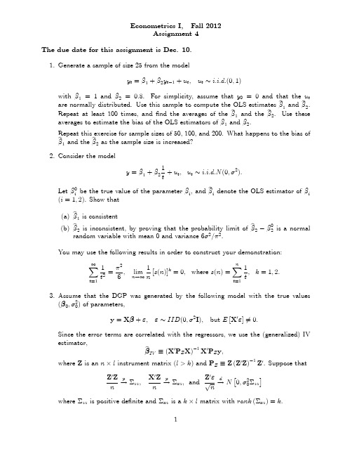
Econometrics I,Fall2012Assignment4The due date for this assignment is Dec.10.1.Generate a sample of size25from the modely t= 1+ 2y t 1+u t,u t i:i:d:(0;1)with 1=1and 2=0:8.For simplicity,assume that y0=0and that the u t are normally e this sample to compute the OLS estimates b 1and b 2. Repeat at least100times,and…nd the averages of the b 1and the b e these averages to estimate the bias of the OLS estimators of 1and 2.Repeat this exercise for sample sizes of50,100,and200.What happens to the bias ofb 1and the b 2as the sample size is increased?2.Consider the modely= 1+ 21t+u t;u t i:i:d:N(0; 2):Let 0i be the true value of the parameter i;and b i denote the OLS estimator of i (i=1;2).Show that(a)b 1is consistent(b)b 2is inconsistent,by proving that the probability limit of b 2 02is a normalrandom variable with mean0and variance6 2= 2.You may use the following results in order to construct your demonstration:1X t=11t2= 26;lim n!11n[s(n)]k=0;where s(n)=n X t=11t;k=1;2:3.Assume that the DGP was generated by the following model with the true values( 0; 20)of parameters,y=X +"," IID(0; 2I),but E[X0"]=0: Since the error terms are correlated with the regressors,we use the(generalized)IV estimator,b IV (X0P Z X) 1X0P Z y;where Z is an n l instrument matrix(l>k)and P Z Z(Z0Z) 1Z0.Suppose thatZ0Z n p! zz,X0Znp! xz,and Z0"pnd!N 0; 20 zzwhere zz is positive de…nite and xz is a k l matrix with rank( xz)=k.(a)Show that b IV is consistent and asymptotically normally distributed,and that the asymptotic covariance matrix of p n b GIV 0 is 20p lim X0P Z X n 1.(b)Show thats2IV 1n y X b IV 0 y X b IV p! 20:4.Gaver and Geisel(1974)propose two forms of a consumption function:M1:C t= 1+ 2Y t+ 3Y t 1+"t;M2:C t= 1+ 2Y t+ 3C t 1+u t;where C t and Y t are real consumption and disposable income in period t.The…rst model states that consumption responds to changes in income over two periods,whereas the second states that the e¤ects of changes in income on consumption persist for many periods.For the data set of consumption.txt used in Assignment2,test both the speci…cations of a consumption function by using the following procedures:(a)the encompassing approach discussed in the class.(b)the comprehensive approach-the J and J A Tests.(c)Compare your testing results.5.Consider a model with two explanatory variables x and zy= + x+ z+e;and suppose that y and x are measured with errors but z is not,i.e.we observeY=y+u;X=x+v,Z=z;where e,u,v are mean zero,variances 2e; 2u; 2v respectively,and mutually uncorre-lated.Also e,u and v are uncorrelated with y;x;and z.(a)Write the regression on Y;X and Z,Y= + X+ Z+":What is the error term"?Compute Cov(X;").(b)Let Cov(x;z)= , 2x V ar(x)and 2z V ar(z).Compute V ar(Y),Cov(Y;X),and Cov(Y;Z):(c)Compute the probability limits of the OLS estimators b and b .。
金融计量经济学

1. Time series data
2. Cross-sectional data
3. Panel data, a combination of 1. & 2.
• The data may be quantitative (e.g. exchange rates, stock prices), or qualitative.
changes in economic conditions n Forecasting future values of financial
variables and for financial decision-making.
PPT文档演模板
金融计量经济学
Examples of some problems that may be solved by an Econometrician
1. Testing whether financial markets are weak-form informationally efficient.
2. Testing whether the CAPM or APT represent superior models for the determination of returns on risky assets.
3. Measuring and forecasting the volatility of bond returns. 4. Explaining the determinants of bond credit ratings used by the
ratings agencies. 5. Modelling long-term relationships between prices and exchange rates
上财朱杰金融计量经济学6_ReturnPredictability

+ εt , εt
N (0, σ2 ).
Now the indicator variable will be biased in the direction of drift: It = 1 with probability π; 0 with probability 1 π.
µ
where π = Pr(rt > 0) = Φ( σ ) and Φ( ) is the CDF for a standard normal variable π 2 +(1 π )2 c Now CJ = > 1.
2π (1 π )
Consider an example. Take µ = 0.08 and σ = 0.21, then 0.08 c Φ( 0.21 ) = 0.6484. CJ = 1.19.
JZ (SUFE) Financial Econometrics
10/2012
11 / 33
The CJ Test
JZ (SUFE) Financial Econometrics 10/2012 5 / 33
ቤተ መጻሕፍቲ ባይዱ
The Random Walk
The simulated price process for RW1. Take µ = 0.00055, σ = 0.0224 and T = 1, 000.
Figure: The Simulated Price Procss under Random Walk 1
JZ (SUFE)
Financial Econometrics
10/2012
2 / 33
The Random Walk
Consider an asset’ returns rt and rt +k at two dates t and t + k. s De…ne two arbitrary functions f (rt ) and g (rt +k ), suppose that their covariance is zero Cov [f (rt ), g (rt +k )] = 0, (1) where k > 0. If f ( ) and g ( ) are linear, eq. (1) implies that returns are serially uncorrelated, RW3 If f ( ) is unrestricted, but g ( ) is linear, eq. (1) implies a martingale. If both f ( ) and g ( ) are unrestricted, eq. (1) implies returns are mutually independent, RW1 or RW2.
上财高级计量经济学朱东明作业2
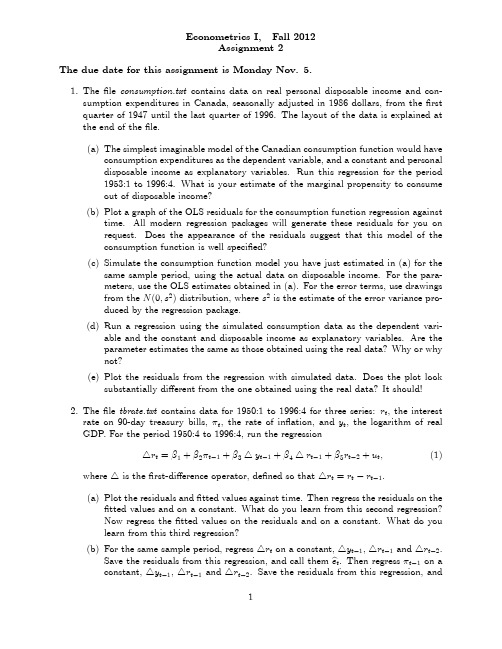
Econometrics I,Fall2012Assignment2The due date for this assignment is Monday Nov.5.1.The…le consumption.txt contains data on real personal disposable income and con-sumption expenditures in Canada,seasonally adjusted in1986dollars,from the…rst quarter of1947until the last quarter of1996.The layout of the data is explained at the end of the…le.(a)The simplest imaginable model of the Canadian consumption function would haveconsumption expenditures as the dependent variable,and a constant and personaldisposable income as explanatory variables.Run this regression for the period1953:1to1996:4.What is your estimate of the marginal propensity to consumeout of disposable income?(b)Plot a graph of the OLS residuals for the consumption function regression againsttime.All modern regression packages will generate these residuals for you onrequest.Does the appearance of the residuals suggest that this model of theconsumption function is well speci…ed?(c)Simulate the consumption function model you have just estimated in(a)for thesame sample period,using the actual data on disposable income.For the para-meters,use the OLS estimates obtained in(a).For the error terms,use drawingsfrom the N(0;s2)distribution,where s2is the estimate of the error variance pro-duced by the regression package.(d)Run a regression using the simulated consumption data as the dependent vari-able and the constant and disposable income as explanatory variables.Are theparameter estimates the same as those obtained using the real data?Why or whynot?(e)Plot the residuals from the regression with simulated data.Does the plot looksubstantially di¤erent from the one obtained using the real data?It should!2.The…le tbrate.txt contains data for1950:1to1996:4for three series:r t,the interestrate on90-day treasury bills, t,the rate of in‡ation,and y t,the logarithm of real GDP.For the period1950:4to1996:4,run the regression4r t= 1+ 2 t 1+ 34y t 1+ 44r t 1+ 5r t 2+u t;(1) where4is the…rst-di¤erence operator,de…ned so that4r t=r t r t 1.(a)Plot the residuals and…tted values against time.Then regress the residuals on the…tted values and on a constant.What do you learn from this second regression?Now regress the…tted values on the residuals and on a constant.What do youlearn from this third regression?(b)For the same sample period,regress4r t on a constant,4y t 1,4r t 1and4r t 2.Save the residuals from this regression,and call them b e t.Then regress t 1on aconstant,4y t 1,4r t 1and4r t 2.Save the residuals from this regression,andcall them b v t .Now regress b e t on b v t .How are the estimated coe¢cient and the residuals from this last regression related to anything that you obtained when you estimated regression (1)?(c)Calculate the diagonal elements of the hat matrix P X for regression (1)anduse them to calculate a measure of leverage,h t X 0t [X 0X ] 1X t ,where X i =(x t;1;:::;x t;k )0.We say that observations for which h t is large have high leverage or are leverage points.A leverage point is not necessarily in‡uential,but it has the potential to be in‡uential.Plot this measure against time.On the basis of this plot,which observations seem to have unusually high leverage?3.Consider the following linear regression:y =X +"=X 1 1+X 2 2+",where y is n 1,X 1is n k 1,X 2is n k 2,X =[X 1;X 2]is n k (k 1+k 2=k <n ),and 0=[ 01; 02].Suppose that X ,X 1and X 2are of full column rank.The OLS estimator b = b 01;b 020are expressed as b = b 1b 2 =(X 0X ) 1X 0y = X 01X 02 [X 1;X 2] 1 X 01X 02 y = X 01X 1X 01X 2X 02X 1X 02X 2 1 X 01y X 02y:(a)Use the formula of partitioned inverse (see A-74,page824)to show thatb 1=[X 01M 2X 1] 1X 01M 2y =[X 01X 1] 1X 01y b 2=[X 02M 1X 2] 1X 02M 1y =[X 02X 2] 1X 02y whereP i X i (X 0i X i ) 1X 0i ,M i I P i ,i =1;2X 1=M 2X 1;y =M 2y ;X 2=M 1X 2;y =M 1y :(b)Note that a square matrix is an orthogonal projection if and only if it is symmetricand e this result to show that P X P 1is an orthogonal projection matrix.What is the trace of P X P 1?(c)Show that any n 1vector z of the form M 1X 2 ,for an arbitrary k 2 1vec-tor ,is left unchanged when premultiplied by P X P 1;that is,show that(P X P 1)M 1X 2 =M 1X 2 .(d)Why do the above results prove that P X P 1=P M 1X 2,where this last matrix denotes the orthogonal projection on to S (M 1X 2)?(e)Consider the following regressions,all to be estimated by OLS:(a)y =X 2 2+u ;(b)P 1y =X 2 2+u ;(c)P 1y =P 1X 2 2+u ;(d)P X y =X 1 1+X 2 2+u ;(e)P X y =X 2 2+u ;(f)M 1y =X 2 2+u ;(g)M 1y =M 1X 2 2+u ;(h)M 1y =X 1 1+M 1X 2 2+u ;(i)M 1y =M 1X 1 1+M 1X 2 2+u ;(j)P X y =M 1X 2 2+u :For which of these regressions are the estimates of 2the same as for the original regression?Why?For which are the residuals the same?Why?。
2022-2022上海财经大学金融硕士(金融分析师)考研详情介绍与经验指上海财经大学金融分析师

2022-2022上海财经大学金融硕士(金融分析师)考研详情介绍与经验指上海财经大学金融分析师原标题:2022-2022上海财经大学金融硕士(金融分析师)考研详情介绍与经验指学院简介历史悠久上海财经大学金融学院的前身为建立于1921年的国立东南大学银行系,是我国高等院校中最早创设的金融学科之一,学科创始人杨荫薄、朱斯煌等教授为近代中国金融学的奠基人。
建国后,彭信威、刘絜敖、朱元、吴国隽、王宏儒、龚浩成、谢树森、王学青、俞文青等资深教授均对新中国金融高等教育的发展有重要贡献。
1998年,为了适应我国金融事业发展的需要,进一步促进金融学科发展,上海财经大学成立了金融学院,这也是我国大陆高校中设立的第一个金融学院。
体系完整金融学院设有银行系、保险系、国际金融系、证券期货系以及公司金融系共5个系,现有本科四个专业、四个学术型硕士点、两个专业学位硕士点和四个博士点。
凭借学院优良的基础设施、资深的师资团队以及现代化的管理方式和国际化视野,成就了一批批活跃于金融界的学术和实践人才。
师资雄厚学院拥有一流的师资队伍,现有专职教师74人,其中教授26人,副教授25人。
获得博士学位的教师人数超过全体教师比例的89%,其中30位教师获得海外博士学位。
近年来学院注重从国外引进高层次科研与教学人才,现有常任轨教师24人,均具有海外博士学位。
学院还聘请多名海外著名高校的知名学者担任特聘教授,聘请海内外大型金融企业负责人担任兼职教授。
近三年来,学院共有十多名教师参加"国家留基委"项目、学校双语师资培训项目以及美国富布莱特基金资助项目,均提高了教师的研究和教学能力。
金融学院致力于构建一支具有国际视野和较高科研水平的一流师资队伍,以培养具备批判思维能力、创造力和前瞻力的国际化高素质金融专业人才,致力于在中短期内,使学院成为亚洲一流、有一定国际影响力的金融教学、科研基地。
现任院长为美国哥伦比亚大学金融系主任王能教授。
- 1、下载文档前请自行甄别文档内容的完整性,平台不提供额外的编辑、内容补充、找答案等附加服务。
- 2、"仅部分预览"的文档,不可在线预览部分如存在完整性等问题,可反馈申请退款(可完整预览的文档不适用该条件!)。
- 3、如文档侵犯您的权益,请联系客服反馈,我们会尽快为您处理(人工客服工作时间:9:00-18:30)。
If f (x ) is a convex function, then f (E [x ]) 6 E [f (x )] If f (x ) is a concave function, then f (E [x ]) > E [f (x )] Example, f (x ) = e x is a convex function, thus we have e E [x ] 6 E [ e x ] . (6) (5)
The simple gross return between date t
1 and t is de…ned as 1 + Rt . k to date t is
The gross return over k periods from date t
1 + Rt (k ) = (1 + Rt )(1 + Rt 1 ) (1 + Rt k +1 ) Pt Pt 1 Pt k +1 Pt = = . Pt 1 Pt 2 Pt k Pt k The simple net return over k periods is just Rt (k ). These multiperiod returns Rt (k ) are called compound return.
JZ (SUFE) Financial Econometrics 10/2012
(2)
2 / 24
Returns
We need to specify the return horizon in order to compare di¤erent returns. Annualized return: Annualized Rt (k )g = [ ∏ (1 + Rt
Financial Econometrics
Zhu, Jie
Shanghai University of Finance and Economics
October 2012
JZ (SUFE)Fra bibliotekFinancial Econometrics
10/2012
1 / 24
Returns
Denote by Pt the price of an asset at date t with no dividend. The simple net return Rt between dates t Rt = Pt Pt 1 1. 1 and t is de…ned as (1)
(X
σ4 x
µ )4
].
(14)
The quantity K (x ) 3 is called the excess kurtosis. For normal distributions, K (x ) = 3. The positive excess kurtosis means that the random sample from the distribution tends to contain more extreme values compared to the normal distribution.
JZ (SUFE)
Financial Econometrics
10/2012
10 / 24
Distribution of Returns
Now consider a joint distribution function for fRi 1 , ..., RiT g, F (Ri 1 , ...RiT ; θ). We may rewrite F (Ri 1 , ...RiT ; θ) as the product of conditional distributions: F (Ri 1 , ...RiT ; θ) = F (Ri 1 )F (Ri 2 jRi 1 ) F (RiT jRi ,T
Consider a collection of N assets at date t, each with return Rit , where t = 1, ..., T . The most general model is its joint distribution function: F (R11 , ..., RN 1; R12, ...RN 2 ; ...; RN 1, ..., RNT ; x; θ), (20)
where x denotes state variables and θ represents the parameter vector. In practice, the model of (20) is too general. The CAPM considers the joint distribution of the cross section of returns, fR1t , ..., RNt g. Other models focus on the dynamic process of individual asset returns, fRi 1 , ..., RiT g, the time series of returns.
JZ (SUFE) Financial Econometrics 10/2012 7 / 24
Estimation
Estimation of skewness and kurtosis. Let fx1 , ..., xT g be a random sample of X with T observations. The sample mean: 1 T b (15) µ= ∑ xt . T t =1 The sample variance: b σ2 = b S= b K = 1 T ∑ (xt T t =1 b µ )2 . b µ )3 . b µ )4 . (16)
The estimated variances 6/T b S t = p6/T and
The Jarque-Bera normality test statistic: JB =
b b S and K 3 are distributed normally and have and 24/T respectively, thus the t-statistics are b t = pK 3 . 24/T b b S2 (K 3)2 + . 6/T 24/T (19)
= log(1 + Rt ) + log(1 + Rt = rt + rt 1 + + rt k +1 .
1) +
(1 + Rt + log(1 + Rt k +1 )
1)
k +1 ))
(8)
2. rt has no constrained lower limit - make it easier to apply to statistical analysis. The disadvantage of log return: For a portfolio, it holds that Rpt = ∑ wi Rit , but it only holds
JZ (SUFE)
R0t . r0t .
10/2012
(11)
(12)
6 / 24
Financial Econometrics
Skewness and Kurtosis
The …rst two moments can uniquely determine a normal distribution. The third central moment measures the symmetry of X with respect to its mean. The standardized third central moment is called skewness: (X µ )3 S (x ) = E [ ]. (13) σ3 x The standardized fourth central moment is called kurtosis, it measures the tail behavior of X : K (x ) = E [
Annualized Rt (k ) Rt (k ) is called the arithmetic average. We can show that Rt (k )g 6 Rt (k ).
JZ (SUFE) Financial Econometrics
(4)
10/2012
3 / 24
Jensen Inequality
1 , ..., Ri 1 ). 1 , ..., Ri 1 )
= f (Ri 1 ) ∏ f (Rit jRi ,t
t =2
JZ (SUFE) Financial Econometrics
T
(22)
10/2012
11 / 24
Distribution of Returns
JZ (SUFE)
Financial Econometrics
10/2012
4 / 24
Returns
Continuous compounding (log return): rt = log(1 + Rt ) = log Pt = pt Pt 1 pt
1.
(7)
The advantage of log return: 1. It is easy to calculate multiperiod return: rt (k ) = log(1 + Rt (k )) = log((1 + Rt )(1 + Rt
1 , ..., Ri 1 ). 1 , ..., Ri 1 )