Finds算法_matlab版本
matlab距离判别法
matlab距离判别法
距离判别法是一种常见的模式识别方法,用于将输入样本分配到已知的类别中。
在MATLAB中,可以使用以下函数来实现
距离判别法:
1. pdist2:计算两个矩阵之间的距离。
例如,可以使用`D = pdist2(X, Y)`计算矩阵X中每个样本与矩阵Y中每个样本之间
的欧氏距离。
2. knnsearch:在给定查询点集和参考点集之间查找最近邻。
例如,可以使用`[IDX, D] = knnsearch(X, Y)`找到矩阵Y中每
个样本的最近邻索引和距离。
3. classify:使用各类训练样本和它们的标签,对测试样本进
行分类。
例如,可以使用`predicted_labels =
classify(test_samples, train_samples, train_labels)`对测试样本进
行分类,并返回预测的标签。
4. fitcknn:用于训练K最近邻(K-Nearest Neighbor)分类器。
例如,可以使用`Mdl = fitcknn(train_samples, train_labels)`训练
一个KNN分类器。
这些函数提供了一些基本的工具来实现距离判别法,但具体的实现取决于你的数据和实际问题。
你可以根据自己的需要选择合适的函数,设置适当的参数,并编写相应的代码。
MATLAB编程基础入门教程
MATLAB编程基础入门教程Chapter 1: Introduction to MATLAB ProgrammingMATLAB is a widely used programming language and environment that is specifically designed for numerical computing. In this chapter, we will provide a comprehensive introduction to MATLAB programming and its fundamental concepts.1.1 MATLAB EnvironmentMATLAB provides an interactive environment where users can write and execute their programs. It offers a user-friendly interface that includes a command window, an editor, and a workspace. The command window allows users to execute commands directly and see the output instantly. The editor is used to write and save MATLAB programs, while the workspace displays the variables and their values.1.2 Variables and Data TypesIn MATLAB, variables are used to store data. They can be assigned values of different data types, including numeric data types such as integers, floating-point numbers, and complex numbers. MATLAB also supports character and string data types. Understanding data types is crucial for performing accurate calculations and data manipulations.1.3 Basic OperationsMATLAB supports a wide range of arithmetic and logical operations. Users can perform basic operations such as addition,subtraction, multiplication, and division on both scalars and arrays. MATLAB also provides functions for more complex mathematical operations such as exponentiation, logarithm, and trigonometric functions.1.4 Control Flow StatementsControl flow statements allow users to control the flow of program execution. MATLAB supports various control flow statements, including if-else statements, for loops, while loops, and switch statements. These statements enable users to write programs that can make decisions or repeat steps based on certain conditions.Chapter 2: MATLAB Programming TechniquesIn this chapter, we will delve deeper into MATLAB programming techniques that will enhance the efficiency and readability of your code.2.1 Functions and ScriptsFunctions and scripts are two fundamental components of MATLAB programming. Functions are reusable pieces of code that accept inputs and produce outputs. They allow for modular and organized programming. Scripts, on the other hand, are collections of code that execute in a specific order. They are useful for automating a series of commands or calculations.2.2 File I/O OperationsMATLAB provides functions to read and write data from and to different file formats. These file I/O operations are crucial for data analysis and processing tasks. MATLAB supports file formats such as text files, spreadsheets, images, and audio files. Understanding how to efficiently read and write data from different file formats will greatly enhance your data processing capabilities.2.3 Error HandlingError handling is an essential aspect of programming. MATLAB provides mechanisms to catch and handle errors that may occur during program execution. By implementing proper error handling techniques, you can make your code more robust and prevent unexpected crashes or undesired outcomes.2.4 Debugging and ProfilingDebugging is the process of identifying and fixing errors or bugs in your code. MATLAB provides debugging tools that allow you to step through your code, set breakpoints, and inspect variables. Profiling, on the other hand, helps identify code bottlenecks and optimize the performance of your programs. Profiling tools provide insights into the execution time and memory usage of different parts of your code.Chapter 3: MATLAB Graphics and VisualizationMATLAB offers powerful tools for creating highly visual and interactive graphics. In this chapter, we will explore MATLAB'sgraphics capabilities and techniques for creating professional-quality visualizations.3.1 Basic PlottingMATLAB provides functions for creating basic 2D and 3D plots. Users can plot data points, lines, surfaces, and volumes. They can also customize the appearance of plots by changing colors, line styles, and markers. Understanding how to create and customize basic plots will enable you to effectively visualize your data.3.2 Advanced Plotting TechniquesMATLAB's advanced plotting techniques allow users to create more complex visualizations. These techniques include plotting multiple data sets on the same graph, adding legends and labels, creating subplots, and customizing axes properties. By mastering these techniques, you can generate informative and aesthetically pleasing visualizations.3.3 Animation and Interactive GraphicsMATLAB provides tools for creating animations and interactive graphics. Animation allows you to visualize changes in data over time. Interactive graphics enable users to interact with plots by zooming, panning, or selecting data points. Understanding how to create animations and interactive graphics will enhance the engagement and effectiveness of your visualizations.Chapter 4: MATLAB Applications and ExtensionsMATLAB offers a wide range of toolboxes and extensions that extend its functionality and allow users to solve specific technical problems. In this chapter, we will explore some popular MATLAB toolboxes and their applications.4.1 Signal Processing ToolboxThe Signal Processing Toolbox provides functions for analyzing and processing signals. It offers tools for filtering, spectral analysis, time-frequency analysis, and wavelet analysis. This toolbox is widely used in fields such as telecommunications, audio processing, and biomedical engineering.4.2 Image Processing ToolboxThe Image Processing Toolbox is designed for image analysis and manipulation tasks. It offers functions for image enhancement, segmentation, morphological operations, and spatial transformations. This toolbox finds applications in fields such as medical imaging, computer vision, and remote sensing.4.3 Control System ToolboxThe Control System Toolbox provides tools for analyzing and designing control systems. It offers functions for modeling, simulation, and control system design. This toolbox is valuable for engineers working in fields such as robotics, aerospace, and industrial automation.4.4 Machine Learning ToolboxThe Machine Learning Toolbox enables users to implement various machine learning algorithms. It provides functions for classification, regression, clustering, and dimensionality reduction. This toolbox is widely used in data analysis, pattern recognition, and predictive modeling.Conclusion:MATLAB is a powerful and versatile programming language for numerical computing. In this tutorial, we have covered the essential concepts and techniques required for getting started with MATLAB programming. By mastering these foundation skills, you can explore more advanced topics and unlock the full potential of MATLAB as a tool for technical computation and data visualization.。
MATLAB教程-台大郭彦甫-11

A function handle
Initial guess
Applications of MATLAB in Engineering
Y.-F. Kuo
14
Exercise
• Find the root for this equation :
2������ − ������ − ������ −������ ������ ������, ������ = −������ + 2������ − ������ −������
Applications of MATLAB in Engineering
Y.-F. Kuo
11
Review of Function Handles (@)
• A handle is a pointer to a function • Can be used to pass functions to other functions
• Try: xy_plot(@sin,0:0.01:2*pi);
Applications of MATLAB in Engineering
Y.-F. Kuo
12
Using Function Handles
xy_plot(@sin,0:0.01:2*pi); xy_plot(@atan,0:0.01:2*pi);
Applications of MATLAB in Engineering
Y.-F. Kuo
16
Finding Roots of Polynomials: roots()
• Find the roots of this polynomial:
������(������) = ������5 − 3.5������4 + 2.75������3 + 2.125������2 − 3.875������ + 1.25
Matlab的标记分水岭分割算法
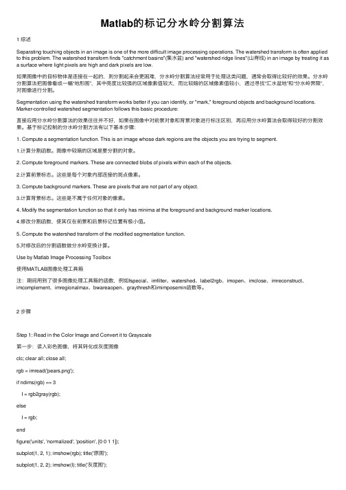
Matlab的标记分⽔岭分割算法1 综述Separating touching objects in an image is one of the more difficult image processing operations. The watershed transform is often applied to this problem. The watershed transform finds "catchment basins"(集⽔盆) and "watershed ridge lines"(⼭脊线) in an image by treating it as a surface where light pixels are high and dark pixels are low.如果图像中的⽬标物体是连接在⼀起的,则分割起来会更困难,分⽔岭分割算法经常⽤于处理这类问题,通常会取得⽐较好的效果。
分⽔岭分割算法把图像看成⼀幅“地形图”,其中亮度⽐较强的区域像素值较⼤,⽽⽐较暗的区域像素值较⼩,通过寻找“汇⽔盆地”和“分⽔岭界限”,对图像进⾏分割。
Segmentation using the watershed transform works better if you can identify, or "mark," foreground objects and background locations. Marker-controlled watershed segmentation follows this basic procedure:直接应⽤分⽔岭分割算法的效果往往并不好,如果在图像中对前景对象和背景对象进⾏标注区别,再应⽤分⽔岭算法会取得较好的分割效果。
基于标记控制的分⽔岭分割⽅法有以下基本步骤:1. Compute a segmentation function. This is an image whose dark regions are the objects you are trying to segment.1.计算分割函数。
手把手教你在Matlab中实现机器学习算法

手把手教你在Matlab中实现机器学习算法机器学习是一门应用统计学、人工智能和计算机科学的交叉学科,旨在使计算机能够从数据中学习并自动执行任务。
在过去的几十年中,机器学习已经取得了巨大的突破,并在各种领域产生了广泛的应用。
Matlab作为一种强大的科学计算软件,提供了丰富的函数和工具包,可以方便地实现各种机器学习算法。
本文将手把手地教你在Matlab中实现机器学习算法。
在开始之前,我们需要准备一些数据。
机器学习算法通常需要大量的数据来训练和测试。
你可以在互联网上找到一些公开的数据集,也可以自己收集和处理数据。
为了方便起见,我们在这里使用一个简单的示例数据集。
我们的示例数据集是一个关于房价的数据集,包含了一些房屋的特征(如面积、位置等)和对应的房价。
我们的目标是根据这些特征来预测房价。
现在,让我们加载数据集并进行一些基本的数据处理。
首先,我们需要将数据集划分为训练集和测试集。
训练集用于训练机器学习模型,而测试集用于评估模型的性能。
在Matlab中,你可以使用`cvpartition`函数来实现数据集的划分。
```matlabload house_dataset.matcv = cvpartition(size(features,1),'HoldOut',0.3);idx = cv.test;train_features = features(~idx,:);train_labels = labels(~idx,:);test_features = features(idx,:);test_labels = labels(idx,:);```接下来,我们需要对数据进行预处理。
预处理步骤可以帮助提取有用的特征,并消除数据中的噪声和冗余。
在这个例子中,我们将对特征进行归一化处理,以确保它们具有相同的尺度。
```matlabtrain_features = normalize(train_features);test_features = normalize(test_features);```完成了数据的划分和预处理后,接下来我们可以开始实现机器学习算法了。
第四章_MATLAB的数值计算功能
第四章MATLAB 的数值计算功能Chapter 4: Numerical computation of MATLAB数值计算是MATLAB最基本、最重要的功能,是MATLAB最具代表性的特点。
MATLAB在数值计算过程中以数组和矩阵为基础。
数组是MATLAB运算中的重要数据组织形式。
前面章节对数组、矩阵的特征及其创建与基本运算规则等相关知识已作了较详尽的介绍,本章重点介绍常用的数值计算方法。
一、多项式(Polynomial)`多项式在众多学科的计算中具有重要的作用,许多方程和定理都是多项式的形式。
MATLAB提供了标准多项式运算的函数,如多项式的求根、求值和微分,还提供了一些用于更高级运算的函数,如曲线拟合和多项式展开等。
1.多项式的表达与创建(Expression and Creating of polynomial)(1) 多项式的表达(expression of polynomial)_Matlab用行矢量表达多项式系数(Coefficient)和根,系数矢量中各元素按变量的降幂顺序排列,如多项式为:P(x)=a0x n+a1x n-1+a2x n-2…a n-1x+a n则其系数矢量(V ector of coefficient)为:P=[a0 a1… a n-1 a n]如将根矢量(V ector of root)表示为:ar=[ ar1 ar2… ar n]则根矢量与系数矢量之间关系为:(x-ar1)(x- ar2) … (x- ar n)= a0x n+a1x n-1+a2x n-2…a n-1x+a n(2)多项式的创建(polynomial creating)a,系数矢量的直接输入法利用poly2sym函数直接输入多项式的系数矢量,就可方便的建立符号形式的多项式。
例1:创建给定的多项式x3-4x2+3x+2poly2sym([1 -4 3 2])ans =x^3-4*x^2+3*x+2也可以用poly2str.求一个方阵对应的符号形式的多项式。
多旅行商问题的matlab程序
%多旅行商问题的matlab程序function varargout = mtspf_gaxy,dmat,salesmen,min_tour,pop_size,num_iter,show_prog,show_res % MTSPF_GA Fixed Multiple Traveling Salesmen Problem M-TSP Genetic Algorithm GA% Finds a near optimal solution to a variation of the M-TSP by setting% up a GA to search for the shortest route least distance needed for% each salesman to travel from the start location to individual cities% and back to the original starting place%% Summary:% 1. Each salesman starts at the first point, and ends at the first% point, but travels to a unique set of cities in between% 2. Except for the first, each city is visited by exactly one salesman%% Note: The Fixed Start/End location is taken to be the first XY point%% Input:% XY float is an Nx2 matrix of city locations, where N is the number of cities% DMAT float is an NxN matrix of city-to-city distances or costs% SALESMEN scalar integer is the number of salesmen to visit the cities% MIN_TOUR scalar integer is the minimum tour length for any of the% salesmen, NOT including the start/end point% POP_SIZE scalar integer is the size of the population should be divisible by 8% NUM_ITER scalar integer is the number of desired iterations for the algorithm to run% SHOW_PROG scalar logical shows the GA progress if true% SHOW_RES scalar logical shows the GA results if true%% Output:% OPT_RTE integer array is the best route found by the algorithm% OPT_BRK integer array is the list of route break points these specify the indices% into the route used to obtain the individual salesman routes% MIN_DIST scalar float is the total distance traveled by the salesmen%% Route/Breakpoint Details:% If there are 10 cities and 3 salesmen, a possible route/break% combination might be: rte = 5 6 9 4 2 8 10 3 7, brks = 3 7% Taken together, these represent the solution 1 5 6 9 11 4 2 8 11 10 3 7 1,% which designates the routes for the 3 salesmen as follows:% . Salesman 1 travels from city 1 to 5 to 6 to 9 and back to 1% . Salesman 2 travels from city 1 to 4 to 2 to 8 and back to 1% . Salesman 3 travels from city 1 to 10 to 3 to 7 and back to 1%% 2D Example:% n = 35;% xy = 10randn,2;% salesmen = 5;% min_tour = 3;% pop_size = 80;% num_iter = 5e3;% a = meshgrid1:n;% dmat = reshapesqrtsumxya,:-xya',:.^2,2,n,n;% opt_rte,opt_brk,min_dist = mtspf_gaxy,dmat,salesmen,min_tour, ... % pop_size,num_iter,1,1;%% 3D Example:% n = 35;% xyz = 10randn,3;% salesmen = 5;% min_tour = 3;% pop_size = 80;% num_iter = 5e3;% a = meshgrid1:n;% dmat = reshapesqrtsumxyza,:-xyza',:.^2,2,n,n;% opt_rte,opt_brk,min_dist = mtspf_gaxyz,dmat,salesmen,min_tour, ... % pop_size,num_iter,1,1;%% See also: mtsp_ga, mtspo_ga, mtspof_ga, mtspofs_ga, mtspv_ga, distmat %% Author: Joseph Kirk% Email: jdkirk630gmail% Release: 1.3% Release Date: 6/2/09% Process Inputs and Initialize Defaultsnargs = 8;for k = nargin:nargs-1switch kcase 0xy = 10rand40,2;case 1N = sizexy,1;a = meshgrid1:N;dmat = reshapesqrtsumxya,:-xya',:.^2,2,N,N;case 2salesmen = 5;case 3min_tour = 2;case 4pop_size = 80;case 5num_iter = 5e3;case 6show_prog = 1;case 7show_res = 1;otherwiseendend% Verify InputsN,dims = sizexy;nr,nc = sizedmat;if N ~= nr || N ~= ncerror'Invalid XY or DMAT inputs'endn = N - 1; % Separate Start/End City% Sanity Checkssalesmen = max1,minn,roundrealsalesmen1;min_tour = max1,minfloorn/salesmen,roundrealmin_tour1; pop_size = max8,8ceilpop_size1/8;num_iter = max1,roundrealnum_iter1;show_prog = logicalshow_prog1;show_res = logicalshow_res1;% Initializations for Route Break Point Selectionnum_brks = salesmen-1;dof = n - min_toursalesmen; % degrees of freedom addto = ones1,dof+1;for k = 2:num_brksaddto = cumsumaddto;endcum_prob = cumsumaddto/sumaddto;% Initialize the Populationspop_rte = zerospop_size,n; % population of routes pop_brk = zerospop_size,num_brks; % population of breaks for k = 1:pop_sizepop_rtek,: = randpermn+1;pop_brkk,: = randbreaks;end% Select the Colors for the Plotted Routesclr = 1 0 0; 0 0 1; 0.67 0 1; 0 1 0; 1 0.5 0;if salesmen > 5clr = hsvsalesmen;end% Run the GAglobal_min = Inf;total_dist = zeros1,pop_size;dist_history = zeros1,num_iter;tmp_pop_rte = zeros8,n;tmp_pop_brk = zeros8,num_brks;new_pop_rte = zerospop_size,n;new_pop_brk = zerospop_size,num_brks;if show_progpfig = figure'Name','MTSPF_GA | Current Best Solution','Numbertitle','off'; endfor iter = 1:num_iter% Evaluate Members of the Populationfor p = 1:pop_sized = 0;p_rte = pop_rtep,:;p_brk = pop_brkp,:;rng = 1 p_brk+1;p_brk n';for s = 1:salesmend = d + dmat1,p_rterngs,1; % Add Start Distancefor k = rngs,1:rngs,2-1d = d + dmatp_rtek,p_rtek+1;endd = d + dmatp_rterngs,2,1; % Add End Distanceendtotal_distp = d;end% Find the Best Route in the Populationmin_dist,index = mintotal_dist;dist_historyiter = min_dist;if min_dist < global_minglobal_min = min_dist;opt_rte = pop_rteindex,:;opt_brk = pop_brkindex,:;rng = 1 opt_brk+1;opt_brk n';if show_prog% Plot the Best Routefigurepfig;for s = 1:salesmenrte = 1 opt_rterngs,1:rngs,2 1;if dims == 3, plot3xyrte,1,xyrte,2,xyrte,3,'.-','Color',clrs,:;else plotxyrte,1,xyrte,2,'.-','Color',clrs,:; endtitlesprintf'Total Distance = %1.4f, Iteration = %d',min_dist,iter;hold onendif dims == 3, plot3xy1,1,xy1,2,xy1,3,'ko';else plotxy1,1,xy1,2,'ko'; endhold offendend% Genetic Algorithm Operatorsrand_grouping = randpermpop_size;for p = 8:8:pop_sizertes = pop_rterand_groupingp-7:p,:;brks = pop_brkrand_groupingp-7:p,:;dists = total_distrand_groupingp-7:p;ignore,idx = mindists;best_of_8_rte = rtesidx,:;best_of_8_brk = brksidx,:;rte_ins_pts = sortceilnrand1,2;I = rte_ins_pts1;J = rte_ins_pts2;for k = 1:8 % Generate New Solutionstmp_pop_rtek,: = best_of_8_rte;tmp_pop_brkk,: = best_of_8_brk;switch kcase 2 % Fliptmp_pop_rtek,I:J = fliplrtmp_pop_rtek,I:J;case 3 % Swaptmp_pop_rtek,I J = tmp_pop_rtek,J I;case 4 % Slidetmp_pop_rtek,I:J = tmp_pop_rtek,I+1:J I;case 5 % Modify Breakstmp_pop_brkk,: = randbreaks;case 6 % Flip, Modify Breakstmp_pop_rtek,I:J = fliplrtmp_pop_rtek,I:J;tmp_pop_brkk,: = randbreaks;case 7 % Swap, Modify Breakstmp_pop_rtek,I J = tmp_pop_rtek,J I;tmp_pop_brkk,: = randbreaks;case 8 % Slide, Modify Breakstmp_pop_rtek,I:J = tmp_pop_rtek,I+1:J I;tmp_pop_brkk,: = randbreaks;otherwise % Do Nothingendendnew_pop_rtep-7:p,: = tmp_pop_rte;new_pop_brkp-7:p,: = tmp_pop_brk;endpop_rte = new_pop_rte;pop_brk = new_pop_brk;endif show_res% Plotsfigure'Name','MTSPF_GA | Results','Numbertitle','off';subplot2,2,1;if dims == 3, plot3xy:,1,xy:,2,xy:,3,'k.';else plotxy:,1,xy:,2,'k.'; endtitle'City Locations';subplot2,2,2;imagescdmat1 opt_rte,1 opt_rte;title'Distance Matrix';subplot2,2,3;rng = 1 opt_brk+1;opt_brk n';for s = 1:salesmenrte = 1 opt_rterngs,1:rngs,2 1;if dims == 3, plot3xyrte,1,xyrte,2,xyrte,3,'.-','Color',clrs,:;else plotxyrte,1,xyrte,2,'.-','Color',clrs,:; endtitlesprintf'Total Distance = %1.4f',min_dist;hold on;endif dims == 3, plot3xy1,1,xy1,2,xy1,3,'ko';else plotxy1,1,xy1,2,'ko'; endsubplot2,2,4;plotdist_history,'b','LineWidth',2;title'Best Solution History';setgca,'XLim',0 num_iter+1,'YLim',0 1.1max1 dist_history; end% Return Outputsif nargoutvarargout{1} = opt_rte;varargout{2} = opt_brk;varargout{3} = min_dist;end% Generate Random Set of Break Pointsfunction breaks = randbreaksif min_tour == 1 % No Constraints on Breakstmp_brks = randpermn-1;breaks = sorttmp_brks1:num_brks;else % Force Breaks to be at Least the Minimum Tour Length num_adjust = findrand < cum_prob,1-1;spaces = ceilnum_brksrand1,num_adjust;adjust = zeros1,num_brks;for kk = 1:num_brksadjustkk = sumspaces == kk;endbreaks = min_tour1:num_brks + cumsumadjust;endendend。
MATLAB中常见的图像识别算法介绍
MATLAB中常见的图像识别算法介绍图像识别是指利用计算机视觉技术对图像进行分析和处理,从中提取出有用的信息。
MATLAB作为一种强大的计算软件,提供了丰富的图像处理和分析工具,能够支持各种常见的图像识别算法。
在本文中,我们将介绍几种常用的图像识别算法,并探讨其原理和应用。
一、图像特征提取算法图像识别的第一步是提取图像特征,即从图像中提取出能够代表图像内容的信息。
常用的图像特征提取算法包括SIFT(Scale-Invariant Feature Transform)、SURF(Speeded-Up Robust Features)和HOG(Histogram of Oriented Gradients)等。
SIFT算法通过检测图像中的关键点,并计算这些关键点的描述子,从而表示图像的局部特征。
SURF算法是对SIFT算法的一种改进,它具有更快的运算速度和更好的鲁棒性。
HOG算法则通过统计图像中不同方向上的梯度信息来描述图像的纹理特征。
这些图像特征提取算法在图像识别任务中广泛应用,例如人脸识别、物体检测等。
它们的主要优势在于对图像的旋转、尺度和光照变化具有较好的不变性。
二、图像分类算法在提取了图像特征之后,接下来就是将提取到的特征应用于图像分类任务。
常用的图像分类算法有支持向量机(SVM)、K最近邻(KNN)和深度学习等。
支持向量机是一种经典的机器学习算法,在图像分类中有着广泛的应用。
它通过寻找一个最优的超平面来将不同类别的样本分开。
支持向量机具有较好的泛化能力,能够处理高维特征,对于非线性问题也能够通过核技巧进行处理。
K最近邻算法则是一种简单而有效的分类方法。
它基于样本的邻近性,将测试样本分类为最近邻居中的多数类别。
KNN算法的优势在于对于训练数据没有假设,但存在计算复杂度高和决策边界不平滑等问题。
深度学习是近年来兴起的一种机器学习方法,通过神经网络模型对图像进行表征学习和分类。
深度学习在图像识别领域取得了重大突破,其中卷积神经网络(CNN)是其重要的代表。
Matlab函数大全
Matlab函数大全matlab常用命令参考1、学会用hel p和doc函数。
2、输入输出文件:save/load在屏幕上显示文件:type3、解线性方程组AX=B:X=A\B4、作图时两张曲线合并:hold on或者su bplot作子图5、程序计算时间:tic,toc或者c lock6、变量显示方式更改:format long/short/bank...7、数组元素求和:sum8、求数组长度:length求矩阵维数:size或者ndims矩阵元素个数:numel9、函数作图:饼图:pie/pie3 误差图:errorb ar 散点图:scatte r/scatte r3 直方图:hist 函数图:fplot动画:movie10、矩阵分析:左右翻转:fliplr上下翻转:flipud转置:transp ose矩阵求逆:inv 矩阵范数:norm 条件数:cond初等变换:rref 特征值:eig/eigs11、特殊矩阵:元素全为1的矩阵:ones 元素全为0的矩阵:zeros单位阵:eye 魔方阵:magic线性变化数组:linspa ce 聚合矩阵:cat/horzca t/vertca t12、随机数:创建一个元素服从均匀分布的随机数数组:rand创建一个元素服从正态分布的随机数数组:randn二项分布:binorn d 指数分布:exprnd F分布:frnd几何分布:geornd超几何分布:hygern d 泊松分布:poissr nd正态分布:normrn d 离散均匀分布:unidrn d 连续均匀分布:unifrn d13、清屏:clc 清理内存:clear14、字体显示变更等:prefer ences15、得到一个文件夹的所有文件名:ls信源函数rander r 产生比特误差样本randin t 产生均匀分布的随机整数矩阵randsr c 根据给定的数字表产生随机矩阵wgn 产生高斯白噪声信号分析函数biterr计算比特误差数和比特误差率eyedia gram绘制眼图scatte rplot绘制分布图symerr计算符号误差数和符号误差率信源编码compan d mu律/A律压缩/扩张dpcmde co DPCM(差分脉冲编码调制)解码dpcmen co DPCM编码dpcmop t 优化DPCM参数lloyds Lloyd法则优化量化器参数quanti z 给出量化后的级和输出值误差控制编码bchpol y 给出二进制B CH码的性能参数和产生多项式conven c 产生卷积码cyclge n 产生循环码的奇偶校验阵和生成矩阵cyclpo ly 产生循环码的生成多项式decode分组码解码器encode分组码编码器gen2pa r 将奇偶校验阵和生成矩阵互相转换gfweig ht 计算线性分组码的最小距离hammge n 产生汉明码的奇偶校验阵和生成矩阵rsdeco f 对Reed-Solomo n编码的A SCII文件解码rsenco f 用Reed-Solomo n码对AS CII文件编码rspoly给出Reed-Solomo n码的生成多项式syndta ble 产生伴随解码表vitdec用Viter bi法则解卷积码(误差控制编码的低级函数)bchdec o BCH解码器bchenc o BCH编码器rsdeco Reed-Solomo n解码器rsdeco de 用指数形式进行Reed-Solomo n解码rsenco Reed-Solomo n编码器rsenco de 用指数形式进行Reed-Solomo n编码调制与解调ademod模拟通带解调器ademod ce 模拟基带解调器amod 模拟通带调制器amodce模拟基带调制器apkcon st 绘制圆形的复合ASK-PSK星座图ddemod数字通带解调器ddemod ce 数字基带解调器demodm ap 解调后的模拟信号星座图反映射到数字信号dmod 数字通带调制器dmodce数字基带调制器modmap把数字信号映射到模拟信号星座图(以供调制)qaskde co 从方形的QA SK星座图反映射到数字信号qasken co 把数字信号映射到方形的QASK星座图专用滤波器hank2s ys 把一个Han kel矩阵转换成一个线性系统模型hilbii r 设计一个希尔伯特变换I IR滤波器rcosfl t 升余弦滤波器rcosin e 设计一个升余弦滤波器(专用滤波器的低级函数)rcosfi r 设计一个升余弦FIR滤波器rcosii r 设计一个升余弦IIR滤波器信道函数awgn 添加高斯白噪声伽罗域计算gfadd伽罗域上的多项式加法gfconv伽罗域上的多项式乘法gfcose ts 生成伽罗域的分圆陪集gfdeco nv 伽罗域上的多项式除法gfdiv伽罗域上的元素除法gffilt er 在质伽罗域上用多项式过滤数据gfline q 在至伽罗域上求Ax=b的一个特解gfminp ol 求伽罗域上元素的最小多项式gfmul伽罗域上的元素乘法gfplus GF(2^m)上的元素加法gfpret ty 以通常方式显示多项式gfprim ck 检测多项式是否是基本多项式gfprim df 给出伽罗域的MATLA B默认的基本多项式gfprim fd 给出伽罗域的基本多项式gfrank伽罗域上矩阵求秩gfrepc ov GF(2)上多项式的表达方式转换gfroot s 质伽罗域上的多项式求根gfsub伽罗域上的多项式减法gftrun c 使多项式的表达最简化gftupl e 简化或转换伽罗域上元素的形式工具函数bi2de把二进制向量转换成十进制数de2bi把十进制数转换成二进制向量erf 误差函数erfc 余误差函数istrel lis 检测输入是否MATLA B的tre llis结构(struct ure)marcum q 通用Marc um Q 函数oct2de c 八进制数转十进制数poly2t relli s 把卷积码多项式转换成M ATLAB的trel lis描述vec2ma t 把向量转换成矩阵——————————————————————————————————————————————————A aabs 绝对值、模、字符的ASC II码值acos 反余弦acosh反双曲余弦acot 反余切acoth反双曲余切acsc 反余割acsch反双曲余割align启动图形对象几何位置排列工具all 所有元素非零为真angle相角ans 表达式计算结果的缺省变量名any 所有元素非全零为真area 面域图argnam es 函数M文件宗量名asec 反正割asech反双曲正割asin 反正弦asinh反双曲正弦assign in 向变量赋值atan 反正切atan2四象限反正切atanh反双曲正切autumn红黄调秋色图阵axes 创建轴对象的低层指令axis 控制轴刻度和风格的高层指令B bbar 二维直方图bar3 三维直方图bar3h三维水平直方图barh 二维水平直方图base2d ec X进制转换为十进制bin2de c 二进制转换为十进制blanks创建空格串bone 蓝色调黑白色图阵box 框状坐标轴breakwhile或for 环中断指令bright en 亮度控制C ccaptur e (3版以前)捕获当前图形cart2p ol 直角坐标变为极或柱坐标cart2s ph 直角坐标变为球坐标cat 串接成高维数组caxis色标尺刻度cd 指定当前目录cdedit启动用户菜单、控件回调函数设计工具cdf2rd f 复数特征值对角阵转为实数块对角阵ceil 向正无穷取整cell 创建元胞数组cell2s truct元胞数组转换为构架数组celldi sp 显示元胞数组内容cellpl ot 元胞数组内部结构图示char 把数值、符号、内联类转换为字符对象chi2cd f 分布累计概率函数chi2in v 分布逆累计概率函数chi2pd f 分布概率密度函数chi2rn d 分布随机数发生器chol Choles ky分解clabel等位线标识cla 清除当前轴class获知对象类别或创建对象clc 清除指令窗clear清除内存变量和函数clf 清除图对象clock时钟colorc ube 三浓淡多彩交叉色图矩阵colord ef 设置色彩缺省值colorm ap 色图colspa ce 列空间的基close关闭指定窗口colper m 列排序置换向量comet彗星状轨迹图comet3三维彗星轨迹图compas s 射线图compos e 求复合函数cond (逆)条件数condei g 计算特征值、特征向量同时给出条件数condes t 范-1条件数估计conj 复数共轭contou r 等位线contou rf 填色等位线contou r3 三维等位线contou rslic e 四维切片等位线图conv 多项式乘、卷积cool 青紫调冷色图copper古铜调色图cos 余弦cosh 双曲余弦cot 余切coth 双曲余切cplxpa ir 复数共轭成对排列csc 余割csch 双曲余割cumsum元素累计和cumtra pz 累计梯形积分cylind er 创建圆柱D ddblqua d 二重数值积分deal 分配宗量deblan k 删去串尾部的空格符dec2ba se 十进制转换为X进制dec2bi n 十进制转换为二进制dec2he x 十进制转换为十六进制deconv多项式除、解卷delaun ay Delaun ay 三角剖分del2 离散Lapl acian差分demo Matlab演示det 行列式diag 矩阵对角元素提取、创建对角阵diaryMatlab指令窗文本内容记录diff 数值差分、符号微分digits符号计算中设置符号数值的精度dir 目录列表disp 显示数组displa y 显示对象内容的重载函数dlinmo d 离散系统的线性化模型dmperm矩阵Dulm age-Mendel sohn分解dos 执行DOS指令并返回结果double把其他类型对象转换为双精度数值drawno w 更新事件队列强迫Mat lab刷新屏幕dsolve符号计算解微分方程E eecho M文件被执行指令的显示edit 启动M文件编辑器eig 求特征值和特征向量eigs 求指定的几个特征值end 控制流FOR等结构体的结尾元素下标eps 浮点相对精度error显示出错信息并中断执行errort rap 错误发生后程序是否继续执行的控制erf 误差函数erfc 误差补函数erfcx刻度误差补函数erfinv逆误差函数errorb ar 带误差限的曲线图etreep lot 画消去树eval 串演算指令evalin跨空间串演算指令exist检查变量或函数是否已定义exit 退出Matl ab环境exp 指数函数expand符号计算中的展开操作expint指数积分函数expm 常用矩阵指数函数expm1Pade法求矩阵指数expm2Taylor法求矩阵指数expm3特征值分解法求矩阵指数eye 单位阵ezcont our 画等位线的简捷指令ezcont ourf画填色等位线的简捷指令ezgrap h3 画表面图的通用简捷指令ezmesh画网线图的简捷指令ezmesh c 画带等位线的网线图的简捷指令ezplot画二维曲线的简捷指令ezplot3 画三维曲线的简捷指令ezpola r 画极坐标图的简捷指令ezsurf画表面图的简捷指令ezsurf c 画带等位线的表面图的简捷指令F ffactor符号计算的因式分解feathe r 羽毛图feedba ck 反馈连接feval执行由串指定的函数fft 离散Four ier变换fft2 二维离散Fo urier变换fftn 高维离散Fo urier变换fftshi ft 直流分量对中的谱fieldn ames构架域名figure创建图形窗fill3三维多边形填色图find 寻找非零元素下标findob j 寻找具有指定属性的对象图柄findst r 寻找短串的起始字符下标findsy m 机器确定内存中的符号变量finver se 符号计算中求反函数fix 向零取整flag 红白蓝黑交错色图阵fliplr矩阵的左右翻转flipud矩阵的上下翻转flipdi m 矩阵沿指定维翻转floor向负无穷取整flops浮点运算次数flow Matlab提供的演示数据fmin 求单变量非线性函数极小值点(旧版)fminbn d 求单变量非线性函数极小值点fmins单纯形法求多变量函数极小值点(旧版)fminun c 拟牛顿法求多变量函数极小值点fminse arch单纯形法求多变量函数极小值点fnder对样条函数求导fnint利用样条函数求积分fnval计算样条函数区间内任意一点的值fnplt绘制样条函数图形fopen打开外部文件for 构成for环用format设置输出格式fourie r Fourie r 变换fplot返函绘图指令fprint f 设置显示格式fread从文件读二进制数据fsolve求多元函数的零点full 把稀疏矩阵转换为非稀疏阵funm 计算一般矩阵函数funtoo l 函数计算器图形用户界面fzero求单变量非线性函数的零点G ggamma函数gammai nc 不完全函数gammal n 函数的对数gca 获得当前轴句柄gcbo 获得正执行"回调"的对象句柄gcf 获得当前图对象句柄gco 获得当前对象句柄geomea n 几何平均值get 获知对象属性getfie ld 获知构架数组的域getfra me 获取影片的帧画面ginput从图形窗获取数据global定义全局变量gplot依图论法则画图gradie nt 近似梯度gray 黑白灰度grid 画分格线gridda ta 规则化数据和曲面拟合gtext由鼠标放置注释文字guide启动图形用户界面交互设计工具H hharmme an 调和平均值help 在线帮助helpwi n 交互式在线帮助helpde sk 打开超文本形式用户指南hex2de c 十六进制转换为十进制hex2nu m 十六进制转换为浮点数hidden透视和消隐开关hilb Hilber t矩阵hist 频数计算或频数直方图histc端点定位频数直方图histfi t 带正态拟合的频数直方图hold 当前图上重画的切换开关horner分解成嵌套形式hot 黑红黄白色图hsv 饱和色图I iif-else-elseif条件分支结构ifft 离散Four ier反变换ifft2二维离散Fo urier反变换ifftn高维离散Fo urier反变换ifftsh ift 直流分量对中的谱的反操作ifouri er Fourie r反变换i, j 缺省的"虚单元"变量ilapla ce Laplac e反变换imag 复数虚部image显示图象images c 显示亮度图象imfinf o 获取图形文件信息imread从文件读取图象imwrit e 把imwri te 把图象写成文件ind2su b 单下标转变为多下标inf 无穷大info MathWo rks公司网点地址inline构造内联函数对象inmem列出内存中的函数名input提示用户输入inputn ame 输入宗量名int 符号积分int2st r 把整数数组转换为串数组interp1 一维插值interp2 二维插值interp3 三维插值interp n N维插值interp ft 利用FFT插值introMatlab自带的入门引导inv 求矩阵逆invhil b Hilber t矩阵的准确逆ipermu te 广义反转置isa 检测是否给定类的对象ischar若是字符串则为真isequa l 若两数组相同则为真isempt y 若是空阵则为真isfini te 若全部元素都有限则为真isfiel d 若是构架域则为真isglob al 若是全局变量则为真ishand le 若是图形句柄则为真ishold若当前图形处于保留状态则为真isieee若计算机执行IEEE规则则为真isinf若是无穷数据则为真islett er 若是英文字母则为真islogi cal 若是逻辑数组则为真ismemb er 检查是否属于指定集isnan若是非数则为真isnume ric 若是数值数组则为真isobje ct 若是对象则为真isprim e 若是质数则为真isreal若是实数则为真isspac e 若是空格则为真isspar se 若是稀疏矩阵则为真isstru ct 若是构架则为真isstud ent 若是Matl ab学生版则为真iztran s 符号计算Z反变换J j , K kjacobi an 符号计算中求Jacob ian 矩阵jet 蓝头红尾饱和色jordan符号计算中获得 Jordan标准型keyboa rd 键盘获得控制权kron Kronec ker乘法规则产生的数组L llaplac e Laplac e变换laster r 显示最新出错信息lastwa rn 显示最新警告信息leasts q 解非线性最小二乘问题(旧版)legend图形图例lighti ng 照明模式line 创建线对象lines采用plot画线色linmod获连续系统的线性化模型linmod2 获连续系统的线性化精良模型linspa ce 线性等分向量ln 矩阵自然对数load 从MA T文件读取变量log 自然对数log10常用对数log2 底为2的对数loglog双对数刻度图形logm 矩阵对数logspa ce 对数分度向量lookfo r 按关键字搜索M文件lower转换为小写字母lsqnon lin 解非线性最小二乘问题lu LU分解M mmad 平均绝对值偏差magic魔方阵maple&nb, sp; 运作 Maple格式指令mat2st r 把数值数组转换成输入形态串数组materi al 材料反射模式max 找向量中最大元素mbuild产生EXE文件编译环境的预设置指令mcc 创建MEX或EXE文件的编译指令mean 求向量元素的平均值median求中位数menued it 启动设计用户菜单的交互式编辑工具mesh 网线图meshz垂帘网线图meshgr id 产生"格点"矩阵method s 获知对指定类定义的所有方法函数mex 产生MEX文件编译环境的预设置指令mfunli s 能被mfun计算的MA PLE经典函数列表mhelp引出 Maple的在线帮助min 找向量中最小元素mkdir创建目录mkpp 逐段多项式数据的明晰化mod 模运算more 指令窗中内容的分页显示movie放映影片动画moviei n 影片帧画面的内存预置mtaylo r 符号计算多变量Tayl or级数展开N nndims求数组维数NaN 非数(预定义)变量nargch k 输入宗量数验证nargin函数输入宗量数nargou t 函数输出宗量数ndgrid产生高维格点矩阵newplo t 准备新的缺省图、轴nextpo w2 取最接近的较大2次幂nnz 矩阵的非零元素总数nonzer os 矩阵的非零元素norm 矩阵或向量范数normcd f 正态分布累计概率密度函数normes t 估计矩阵2范数normin v 正态分布逆累计概率密度函数normpd f 正态分布概率密度函数normrn d 正态随机数发生器notebo ok 启动Matl ab和Wo rd的集成环境null 零空间num2st r 把非整数数组转换为串numden获取最小公分母和相应的分子表达式nzmax指定存放非零元素所需内存O oode1 非Stiff微分方程变步长解算器ode15s Stiff微分方程变步长解算器ode23t适度Stif f 微分方程解算器ode23t b Stiff微分方程解算器ode45非Stiff微分方程变步长解算器odefil e ODE 文件模板odeget获知ODE选项设置参数odepha s2 ODE 输出函数的二维相平面图odepha s3 ODE 输出函数的三维相空间图odeplo t ODE 输出函数的时间轨迹图odepri nt 在Matla b指令窗显示结果odeset创建或改写ODE选项构架参数值ones 全1数组optims et 创建或改写优化泛函指令的选项参数值orient设定图形的排放方式orth 值空间正交化P ppack 收集Matl ab内存碎块扩大内存pagedl g 调出图形排版对话框patch创建块对象path 设置Matl ab搜索路径的指令pathto ol 搜索路径管理器pause暂停pcode创建预解译P码文件pcolor伪彩图peaksMatlab提供的典型三维曲面permut e 广义转置pi (预定义变量)圆周率pie 二维饼图pie3 三维饼图pink 粉红色图矩阵pinv 伪逆plot 平面线图plot3三维线图plotma trix矩阵的散点图plotyy双纵坐标图poissi nv 泊松分布逆累计概率分布函数poissr nd 泊松分布随机数发生器pol2ca rt 极或柱坐标变为直角坐标polar极坐标图poly 矩阵的特征多项式、根集对应的多项式poly2s tr 以习惯方式显示多项式poly2s ym 双精度多项式系数转变为向量符号多项式polyde r 多项式导数polyfi t 数据的多项式拟合polyva l 计算多项式的值polyva lm 计算矩阵多项式pow2 2的幂ppval计算分段多项式pretty以习惯方式显示符号表达式print打印图形或S IMULI NK模型prints ys 以习惯方式显示有理分式prism光谱色图矩阵procre ad 向MAPLE输送计算程序profil e 函数文件性能评估器proped it 图形对象属性编辑器pwd 显示当前工作目录Q qquad 低阶法计算数值积分quad8高阶法计算数值积分(QUADL)quit 推出Matl ab 环境quiver二维方向箭头图quiver3 三维方向箭头图R rrand 产生均匀分布随机数randn产生正态分布随机数randpe rm 随机置换向量range样本极差rank 矩阵的秩rats 有理输出rcond矩阵倒条件数估计real 复数的实部reallo g 在实数域内计算自然对数realpo w 在实数域内计算乘方realsq rt 在实数域内计算平方根realma x 最大正浮点数realmi n 最小正浮点数rectan gle 画"长方框"rem 求余数repmat铺放模块数组reshap e 改变数组维数、大小residu e 部分分式展开return返回ribbon把二维曲线画成三维彩带图rmfiel d 删去构架的域roots求多项式的根rose 数扇形图rot90矩阵旋转90度rotate指定的原点和方向旋转rotate3d 启动三维图形视角的交互设置功能round向最近整数圆整rref 简化矩阵为梯形形式rsf2cs f 实数块对角阵转为复数特征值对角阵rsumsRieman n和S ssave 把内存变量保存为文件scatte r 散点图scatte r3 三维散点图sec 正割sech 双曲正割semilo gx X轴对数刻度坐标图semilo gy Y轴对数刻度坐标图series串联连接set 设置图形对象属性setfie ld 设置构架数组的域setstr将ASCII码转换为字符的旧版指令sign 根据符号取值函数signum符号计算中的符号取值函数sim 运行SIMU LINK模型simget获取SIMU LINK模型设置的仿真参数simple寻找最短形式的符号解simpli fy 符号计算中进行简化操作simset对SIMUL INK模型的仿真参数进行设置simuli nk 启动SIMU LINK模块库浏览器sin 正弦sinh 双曲正弦size 矩阵的大小slice立体切片图solve求代数方程的符号解spallo c 为非零元素配置内存sparse创建稀疏矩阵spconv ert 把外部数据转换为稀疏矩阵spdiag s 稀疏对角阵spfun求非零元素的函数值sph2ca rt 球坐标变为直角坐标sphere产生球面spinma p 色图彩色的周期变化spline样条插值spones用1置换非零元素sprand sym 稀疏随机对称阵sprank结构秩spring紫黄调春色图sprint f 把格式数据写成串spy 画稀疏结构图sqrt 平方根sqrtm方根矩阵squeez e 删去大小为1的"孤维"sscanf按指定格式读串stairs阶梯图std 标准差stem 二维杆图step 阶跃响应指令str2do uble串转换为双精度值str2ma t 创建多行串数组str2nu m 串转换为数strcat接成长串strcmp串比较strjus t 串对齐strmat ch 搜索指定串strncm p 串中前若干字符比较strrep串替换strtok寻找第一间隔符前的内容struct创建构架数组struct2cell把构架转换为元胞数组strvca t 创建多行串数组sub2in d 多下标转换为单下标subexp r 通过子表达式重写符号对象subplo t 创建子图subs 符号计算中的符号变量置换subspa ce 两子空间夹角sum 元素和summer绿黄调夏色图superi orto设定优先级surf 三维着色表面图surfac e 创建面对象surfc带等位线的表面图surfl带光照的三维表面图surfno rm 空间表面的法线svd 奇异值分解svds 求指定的若干奇异值switch-case-otherw ise 多分支结构sym2po ly 符号多项式转变为双精度多项式系数向量symmmd对称最小度排序symrcm反向Cuth ill-McKee排序syms 创建多个符号对象T ttan 正切tanh 双曲正切taylor tool进行Tayl or逼近分析的交互界面text 文字注释tf 创建传递函数对象tic 启动计时器title图名toc 关闭计时器trapz梯形法数值积分treela yout展开树、林treepl ot 画树图tril 下三角阵trim 求系统平衡点trimes h 不规则格点网线图trisur f 不规则格点表面图triu 上三角阵 try-catch控制流中的T ry-catch结构type 显示M文件U uuicont extme nu 创建现场菜单uicont rol 创建用户控件uimenu创建用户菜单unmkpp逐段多项式数据的反明晰化unwrap自然态相角upper转换为大写字母V vvar 方差vararg in 变长度输入宗量vararg out 变长度输出宗量vector ize 使串表达式或内联函数适于数组运算ver 版本信息的获取view 三维图形的视角控制vorono i Vorono i多边形vpa 任意精度(符号类)数值W wwarnin g 显示警告信息what 列出当前目录上的文件whatsn ew 显示Matl ab中 Readme文件的内容which确定函数、文件的位置while控制流中的W hile环结构white全白色图矩阵whiteb g 指定轴的背景色who 列出内存中的变量名whos 列出内存中变量的详细信息winter蓝绿调冬色图worksp ace 启动内存浏览器X x , Y y , Z zxlabel X轴名xor 或非逻辑yesinp ut 智能输入指令ylabel Y轴名zeros全零数组zlabel Z轴名zoom 图形的变焦放大和缩小ztrans符号计算Z变换Matlab中图像函数大全图像增强1. 直方图均衡化的 Matlab实现1.1 imhist函数功能:计算和显示图像的色彩直方图格式:imhist(I,n)i mhist(X,map)说明:imhist(I,n) 其中,n 为指定的灰度级数目,缺省值为256;imhist(X,map) 就算和显示索引色图像X 的直方图,map 为调色板。
matlab寻优算法
matlab寻优算法
MATLAB具有多种寻优算法,用于解决不同类型的优化问题。
其
中包括线性规划、非线性规划、整数规划、全局优化等。
下面我将
从不同角度介绍一些常见的MATLAB寻优算法。
首先,MATLAB提供了许多内置函数用于寻优算法,比如
`fmincon`用于解决有约束的非线性规划问题,`linprog`用于解决
线性规划问题,`ga`用于遗传算法等。
这些函数可以帮助用户快速
解决各种优化问题。
其次,MATLAB还提供了优化工具箱(Optimization Toolbox),其中包含了更多高级的寻优算法,比如序列二次规划(SQP)、内点法、模拟退火算法、粒子群算法等。
这些算法可以应用于复杂的优
化问题,并且可以通过调整参数来进行定制化。
此外,MATLAB还支持混合整数线性规划(MILP)和混合整数非
线性规划(MINLP)等复杂优化问题的求解。
用户可以使用内置函数
或优化工具箱中的函数来处理这些问题。
除了内置的算法和工具箱,MATLAB还支持用户自定义优化算法。
用户可以编写自己的优化函数,并结合MATLAB的其他功能进行求解。
这样可以满足用户特定的优化需求,提高算法的灵活性和适用性。
总的来说,MATLAB提供了丰富的寻优算法和工具,可以满足各
种不同类型的优化问题的求解需求。
用户可以根据具体情况选择合
适的算法,并通过调整参数或自定义算法来解决复杂的优化问题。
希望以上信息能够帮助你更好地了解MATLAB的寻优算法。
- 1、下载文档前请自行甄别文档内容的完整性,平台不提供额外的编辑、内容补充、找答案等附加服务。
- 2、"仅部分预览"的文档,不可在线预览部分如存在完整性等问题,可反馈申请退款(可完整预览的文档不适用该条件!)。
- 3、如文档侵犯您的权益,请联系客服反馈,我们会尽快为您处理(人工客服工作时间:9:00-18:30)。
Find_s算法:matlab语言EnjoySport概念学习任务:--------------------------------------------------------------------------------------------------------------------- %MATLAB-Finds:寻找极大特殊假设%__date__=2015.4.7%__brief__=FIND-S, from 'machine learning' p19%实例集X的属性及其可能取值:Sky{sunny,cloudy,rainy}AirTemp{warm,cold}Humidity{normal,high}Wind{strong,weak}Water{warm.,cool}Forecas{same,change}%实例空间X包含3×2×2×2×2×2=96中不同的实例%假设空间H包含5×4×4×4×4×4=5120种语法不同的假设%语义不同的假设H只有1+4×3×3×3×3×3=973个------------------------------------------------------------------------------------------------------------------共有4个实例:x1 = { 'sunny ', 'warm ', 'nurmal ', 'strong ', 'warm ', 'same ' , 'yes ' };x2 = { 'sunny ', 'warm ', 'high ', 'strong ', 'warm ', 'same ' , 'yes ' };x3 = { 'rainy ', 'cold ', 'high ', 'strong ', 'warm ', 'change ', 'no ' };x4 = { 'sunny ', 'warm ', 'high ', 'strong ', 'cool ', 'change ', 'yes ' };FIND-S算法思想:从H中最特殊假设开始,然后在该假设覆盖正例失败时将其一般化(当一假设能正确地划分一个正例时,称该假设“覆盖”该正例)。
1.将h初始化为H中最特殊假设2.对每个正例x对h的每个属性约束a i如果x满足a i那么不做任何处理否则将h中a i替换为x满足的下一个更一般的约束3. 输出假设h注:输出结果与实例属性有关,但与实例顺序无关!法1:matlab函数为FS输出为:------------------------------------------------------------------------>> FS极大特殊假设h:1 1 0 1 0 0>>-----------------------------------------------------------------------代码:function FS()% %A=[sunny,warm,normal,strong,warm,change yes;% % sunny,warm,high,strong,warm,same yes ;% % rainy,cold,high,strong,warm,change no;% % sunny,warm,high,strong,cold,change yes ];% % 正例用1表示;反例用0表示% %设各种属性的第一种取值为1;第二种取值为2;第三种取值为3;取为?设为0;取空值时设为4h=[4,4,4,4,4,4]; %将h初始化为H中最特殊假设A=[1,1,1,1,1,1,1;1,1,2,1,1,2,1;2,2,2,1,1,1,0;1,1,2,1,2,1,1;];%第三个为反例,其余为正例for i=1:4 %i为行标if A(i,7)==1 %判断A(i,7)是否为正例for j=1:6 %j为列标if h(j)==4 %判断h(j)是否为最特殊假设,即h(j)~=A(i,j)&&h(j)==4h(j)=A(i,j); %将h(j)一般化A(i,j)elseif h(j)~=A(i,j) %判断h(j)是否等于A(i,j),即h(j)~=A(i,j)&&h(j)==0或h(j)~=A(i,j)&&h(j)~=4h(j)=0; %将h(j)一般化最一般假设% 若h(:,j)与A(i,j)取值相同,则跳出,执行下一次循环% elseif h(:,j)==A(i,j)% continue;end %end ifend %end forend %end ifend %end fordisp('极大特殊假设h:');disp(h);法2:matlab函数为FINDS输出为:------------------------------------------------------------------------------------------------------ >> FINDS极大特殊假设h:'sunny ' 'warm ' '? ' 'strong ' '? ' '? '>>------------------------------------------------------------------------------------------------------- 代码:function FINDS()x1 = { 'sunny ', 'warm ', 'nurmal ', 'strong ', 'warm ', 'same ' , 'yes ' };x2 = { 'sunny ', 'warm ', 'high ', 'strong ', 'warm ', 'same ' , 'yes ' };x3 = { 'rainy ', 'cold ', 'high ', 'strong ', 'warm ', 'change ', 'no ' };x4 = { 'sunny ', 'warm ', 'high ', 'strong ', 'cool ', 'change ', 'yes ' };h0 = {'? ','? ','? ','? ','? ','? '};h = { 'None ', 'None ','None ', 'None ', 'None ', 'None ' };h1 = { 'sunny ', 'cold ', 'high ', 'strong ', 'warm ', 'change ' };%h0为最一般假设,h为最特殊假设,h1为某一假设xa = { x1; x2; x3; x4 };xb = { x2; x3; x4; x1 };%xa,xb为某一假设集hx=h;x=xa;for i=1:length(x) %i为行标if strcmpi(x{i}{7},'yes ') %判断x{i}是否为正例for j = 1:length(x{i})-1 %j为列标if strcmpi(hx{j},'None ') %判断hx{j}是否为特殊假设hx{j} = x{i}{j}; % hx{j}泛化为x{i}{j}elseif ~strcmpi(hx{j},x{i}{j}) %判断hx{j}是否与x{i}{j}相等hx{j} = '? '; % hx{j}泛化为一般假设%若hx{j}是否与x{i}{j}相等,则进行下次循环% elseif ~strcmpi(hx{j},x{i}{j})% continue;end %end ifend %end forend %end ifend %end fordisp('极大特殊假设h:');disp(hx);。