dijkstra算法的matlab实现
最短路dijkstra算法Matlab程序
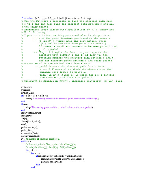
function [c0,c,path0,path]=dijkstra(s,t,C,flag)% Use the Dijkstra's algorithm to find the shortest path from% s to t and can also find the shortest path between s and all% the other points.% Reference: Graph Theory with Applications by J. A. Bondy and% U. S. R. Murty.% Input -- s is the starting point and also is the point s.% -- t is the given terminal point and is the point t.% -- C \in R^{n \times n}is the cost matrix, where% C(i,j)>=0 is the cost from point i to point j.% If there is no direct connection between point i and% j, C(i,j)=inf.% -- flag: if flag=1, the function just reports the% shortest path between s and t; if flag~=1, the% function reports the shortest path between s and t,% and the shortest paths between s and other points.% Output -- c0 is the minimal cost from s to t.% -- path0 denotes the shortest path form s to t.% -- c \in R{1\times n} in which the element i is the% minimal cost from s to point i.% -- path \in R^{n \times n} in which the row i denotes% the shortest path from s to point i.% Copyright by MingHua Xu(徐明华), Changhzou University, 27 Jan. 2014. s=floor(s);t=floor(t);n=size(C,1);if s<1 || t < 1 || s > n || t > nerror(' The starting point and the terminal point exceeds the valid range');endif t==sdisp('The starting point and the terminal point are the same points');endlabel=ones(1,n)*inf;label(s)=0;S=[s];Sbar=[1:s-1,s+1:n];c0=0;path=zeros(n,n);path(:,1)=s;c=ones(1,n)*inf;parent=zeros(1,n);i=1; % number of points in point set S.while i<n% for each point in Sbar, replace label(Sbar(j)) by% min(label(Sbar(j)),label(S(k))+C(S(k),Sbar(j)))for j=1:n-ifor k=1:iif label(Sbar(j)) > label(S(k))+C(S(k),Sbar(j))label(Sbar(j))=label(S(k))+C(S(k),Sbar(j));parent(Sbar(j))=S(k);endendend% Find the minmal label(j), j \in Sbar.temp=label(Sbar(1));son=1;for j=2:n-iif label(Sbar(j))< temptemp=label(Sbar(j));son=j;endend% update the point set S and SbarS=[S,Sbar(son)];Sbar=[Sbar(1:son-1),Sbar(son+1:n-i)];i=i+1;% if flag==1, just output the shortest path between s and t.if flag==1 && S(i)==tson=t;temp_path=[son];if son~=swhile parent(son)~=sson=parent(son);temp_path=[temp_path,son];endtemp_path=[temp_path,s];endtemp_path=fliplr(temp_path);m=size(temp_path,2);path0(1:m)=temp_path;c_temp=0;for j=1:m-1c_temp=c_temp+C(temp_path(j),temp_path(j+1));endc0=c_temp;path(t,1:m)=path0;c(t)=c0;returnendend% Form the output resultsfor i=1:nson=i;temp_path=[son];if son~=swhile parent(son)~=sson=parent(son);temp_path=[temp_path,son];endtemp_path=[temp_path,s];endtemp_path=fliplr(temp_path);m=size(temp_path,2);path(i,1:m)=temp_path;c_temp=0;for j=1:m-1c_temp=c_temp+C(temp_path(j),temp_path(j+1));endc(i)=c_temp;c0=c(t);path0=path(t,:);endreturn。
11基于遗传算法的机器人路径规划MATLAB源代码
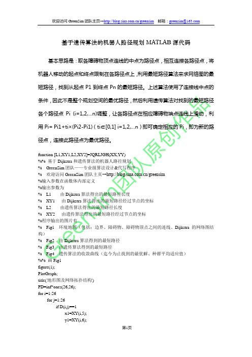
基于遗传算法的机器人路径规划MATLAB源代码基本思路是:取各障碍物顶点连线的中点为路径点,相互连接各路径点,将机器人移动的起点和终点限制在各路径点上,利用最短路径算法来求网络图的最短路径,找到从起点P1到终点Pn的最短路径。
上述算法使用了连接线中点的条件,因此不是整个规划空间的最优路径,然后利用遗传算法对找到的最短路径各个路径点Pi (i=1,2,…n)调整,让各路径点在相应障碍物端点连线上滑动,利用Pi= Pi1+ti×(Pi2-Pi1)(ti∈[0,1] i=1,2,…n)即可确定相应的Pi,即为新的路径点,连接此路径点为最优路径。
function [L1,XY1,L2,XY2]=JQRLJGH(XX,YY)%% 基于Dijkstra和遗传算法的机器人路径规划% GreenSim团队——专业级算法设计&代写程序% 欢迎访问GreenSim团队主页→/greensim%输入参数在函数体内部定义%输出参数为% L1 由Dijkstra算法得出的最短路径长度% XY1 由Dijkstra算法得出的最短路径经过节点的坐标% L2 由遗传算法得出的最短路径长度% XY2 由遗传算法得出的最短路径经过节点的坐标%程序输出的图片有% Fig1 环境地图(包括:边界、障碍物、障碍物顶点之间的连线、Dijkstra的网络图结构)% Fig2 由Dijkstra算法得到的最短路径% Fig3 由遗传算法得到的最短路径% Fig4 遗传算法的收敛曲线(迄今为止找到的最优解、种群平均适应值)%% 画Fig1figure(1);PlotGraph;title('地形图及网络拓扑结构')PD=inf*ones(26,26);for i=1:26for j=1:26if D(i,j)==1x1=XY(i,5);y1=XY(i,6);x2=XY(j,5);y2=XY(j,6);dist=((x1-x2)^2+(y1-y2)^2)^0.5;PD(i,j)=dist;endendend%% 调用最短路算法求最短路s=1;%出发点t=26;%目标点[L,R]=ZuiDuanLu(PD,s,t);L1=L(end);XY1=XY(R,5:6);%% 绘制由最短路算法得到的最短路径figure(2);PlotGraph;hold onfor i=1:(length(R)-1)x1=XY1(i,1);y1=XY1(i,2);x2=XY1(i+1,1);y2=XY1(i+1,2);plot([x1,x2],[y1,y2],'k');hold onendtitle('由Dijkstra算法得到的初始路径')%% 使用遗传算法进一步寻找最短路%第一步:变量初始化M=50;%进化代数设置N=20;%种群规模设置Pm=0.3;%变异概率设置LC1=zeros(1,M);LC2=zeros(1,M);Yp=L1;%第二步:随机产生初始种群X1=XY(R,1);Y1=XY(R,2);X2=XY(R,3);Y2=XY(R,4);for i=1:Nfarm{i}=rand(1,aaa);end% 以下是进化迭代过程counter=0;%设置迭代计数器while counter<M%停止条件为达到最大迭代次数%% 第三步:交叉%交叉采用双亲双子单点交叉newfarm=cell(1,2*N);%用于存储子代的细胞结构Ser=randperm(N);%两两随机配对的配对表A=farm{Ser(1)};%取出父代AB=farm{Ser(2)};%取出父代BP0=unidrnd(aaa-1);%随机选择交叉点a=[A(:,1:P0),B(:,(P0+1):end)];%产生子代ab=[B(:,1:P0),A(:,(P0+1):end)];%产生子代bnewfarm{2*N-1}=a;%加入子代种群newfarm{2*N}=b;for i=1:(N-1)A=farm{Ser(i)};B=farm{Ser(i+1)};newfarm{2*i}=b;endFARM=[farm,newfarm];%新旧种群合并%% 第四步:选择复制SER=randperm(2*N);FITNESS=zeros(1,2*N);fitness=zeros(1,N);for i=1:(2*N)PP=FARM{i};FITNESS(i)=MinFun(PP,X1,X2,Y1,Y2);%调用目标函数endfor i=1:Nf1=FITNESS(SER(2*i-1));f2=FITNESS(SER(2*i));if f1<=f2elsefarm{i}=FARM{SER(2*i)};fitness(i)=FITNESS(SER(2*i));endend%记录最佳个体和收敛曲线minfitness=min(fitness);meanfitness=mean(fitness);if minfitness<Yppos=find(fitness==minfitness);Xp=farm{pos(1)};Yp=minfitness;endif counter==10PPP=[0.5,Xp,0.5]';PPPP=1-PPP;X=PPP.*X1+PPPP.*X2;Y=PPP.*Y1+PPPP.*Y2;XY2=[X,Y];figure(3)PlotGraph;hold onfor i=1:(length(R)-1)x1=XY2(i,1);y1=XY2(i,2);x2=XY2(i+1,1);y2=XY2(i+1,2);plot([x1,x2],[y1,y2],'k');hold onendtitle('遗传算法第10代')hold onfor i=1:(length(R)-1)x1=XY1(i,1);y1=XY1(i,2);x2=XY1(i+1,1);y2=XY1(i+1,2);plot([x1,x2],[y1,y2],'k','LineWidth',1);hold onendendif counter==20PPP=[0.5,Xp,0.5]';PPPP=1-PPP;X=PPP.*X1+PPPP.*X2;Y=PPP.*Y1+PPPP.*Y2;XY2=[X,Y];figure(4)PlotGraph;hold onfor i=1:(length(R)-1)x1=XY2(i,1);y2=XY2(i+1,2);plot([x1,x2],[y1,y2],'k');hold onendtitle('遗传算法第20代')hold onx1=XY1(i,1);y1=XY1(i,2);x2=XY1(i+1,1);y2=XY1(i+1,2);plot([x1,x2],[y1,y2],'k','LineWidth',1);hold onendendif counter==30PPP=[0.5,Xp,0.5]';PPPP=1-PPP;X=PPP.*X1+PPPP.*X2;Y=PPP.*Y1+PPPP.*Y2;XY2=[X,Y];figure(5)PlotGraph;hold onfor i=1:(length(R)-1)x1=XY2(i,1);y1=XY2(i,2);x2=XY2(i+1,1);y2=XY2(i+1,2);plot([x1,x2],[y1,y2],'k');hold onendtitle('遗传算法第30代')hold onfor i=1:(length(R)-1)x1=XY1(i,1);y2=XY1(i+1,2);plot([x1,x2],[y1,y2],'k','LineWidth',1);hold onendendif counter==40PPP=[0.5,Xp,0.5]';PPPP=1-PPP;X=PPP.*X1+PPPP.*X2;Y=PPP.*Y1+PPPP.*Y2;XY2=[X,Y];figure(6)PlotGraph;hold onx1=XY2(i,1);y1=XY2(i,2);x2=XY2(i+1,1);y2=XY2(i+1,2);plot([x1,x2],[y1,y2],'k');hold onendtitle('遗传算法第40代')hold onfor i=1:(length(R)-1)x1=XY1(i,1);y1=XY1(i,2);x2=XY1(i+1,1);y2=XY1(i+1,2);plot([x1,x2],[y1,y2],'k','LineWidth',1);hold onendendif counter==50PPP=[0.5,Xp,0.5]';PPPP=1-PPP;X=PPP.*X1+PPPP.*X2;Y=PPP.*Y1+PPPP.*Y2;XY2=[X,Y];figure(7)PlotGraph;hold onfor i=1:(length(R)-1)x1=XY2(i,1);y1=XY2(i,2);x2=XY2(i+1,1);y2=XY2(i+1,2);plot([x1,x2],[y1,y2],'k');hold onendtitle('遗传算法第50代')hold onfor i=1:(length(R)-1)x1=XY1(i,1);y1=XY1(i,2);x2=XY1(i+1,1);y2=XY1(i+1,2);plot([x1,x2],[y1,y2],'k','LineWidth',1);hold onendendLC2(counter+1)=Yp;LC1(counter+1)=meanfitness;%% 第五步:变异for i=1:Nif Pm>rand&&pos(1)~=iAA=farm{i};AA(POS)=rand;farm{i}=AA;endendcounter=counter+1;disp(counter);end%% 输出遗传算法的优化结果PPP=[0.5,Xp,0.5]';PPPP=1-PPP;X=PPP.*X1+PPPP.*X2;Y=PPP.*Y1+PPPP.*Y2;XY2=[X,Y];L2=Yp;%% 绘制Fig3figure(8)PlotGraph;hold onhold onfor i=1:(length(R)-1)x1=XY1(i,1);y1=XY1(i,2);x2=XY1(i+1,1);y2=XY1(i+1,2);plot([x1,x2],[y1,y2],'k','LineWidth',1);hold onendfor i=1:(length(R)-1)x1=XY2(i,1);y1=XY2(i,2);x2=XY2(i+1,1);y2=XY2(i+1,2);plot([x1,x2],[y1,y2],'k');hold onendtitle('遗传算法最终结果')figure(9)PlotGraph;hold onfor i=1:(length(R)-1)x1=XY1(i,1);y1=XY1(i,2);x2=XY1(i+1,1);y2=XY1(i+1,2);plot([x1,x2],[y1,y2],'k','LineWidth',1);hold onendhold onfor i=1:(length(R)-1)x1=XY2(i,1);y1=XY2(i,2);x2=XY2(i+1,1);y2=XY2(i+1,2);plot([x1,x2],[y1,y2],'k','LineWidth',2);hold onendtitle('遗传算法优化前后结果比较')%% 绘制Fig4figure(10);plot(LC1);hold onplot(LC2);xlabel('迭代次数');title('收敛曲线');源代码运行结果展示。
Dijkstra、Floyd算法Matlab_Lingo实现
Dijkstra算法Matlab实现。
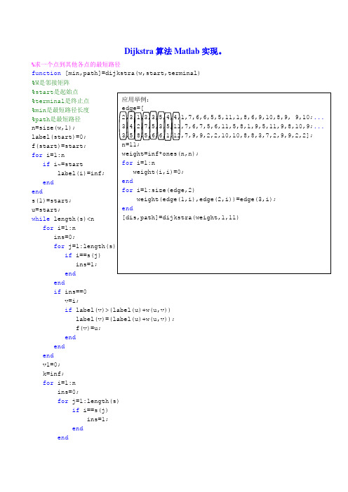
%求一个点到其他各点的最短路径function [min,path]=dijkstra(w,start,terminal)%W是邻接矩阵%start是起始点Array %terminal是终止点%min是最短路径长度%path是最短路径n=size(w,1);label(start)=0;f(start)=start;for i=1:nif i~=startlabel(i)=inf;endends(1)=start;u=start;while length(s)<nfor i=1:nins=0;forif i==s(j)ins=1;endendif ins==0v=i;if label(v)>(label(u)+w(u,v))label(v)=(label(u)+w(u,v));f(v)=u;endendendv1=0;k=inf;for i=1:nins=0;for j=1:length(s)if i==s(j)ins=1;endend-if ins==0v=i;if k>label(v)k=label(v);v1=v;endendends(length(s)+1)=v1;u=v1;endmin=label(terminal);path(1)=terminal;i=1;while path(i)~=startpath(i+1)=f(path(i));i=i+1 ;endpath(i)=start;L=length(path);path=path(L:-1:1);Floyd算法:matlab程序:%floyd算法,function [D,path,min1,path1]=floyd(a,start,terminal)%a是邻接矩阵%start是起始点%terminal是终止点%D是最小权值表D=a;n=size(D,1);path=zeros(n,n);for i=1:nfor j=1:nif D(i,j)~=infpath(i,j)=j;endendendfor k=1:nfor i=1:nfor j=1:nif D(i,k)+D(k,j)<D(i,j)-D(i,j)=D(i,k)+D(k,j);path(i,j)=path(i,k);endendendendif nargin==3min1=D(start,terminal);m(1)=start;i=1;path1=[ ];while path(m(i),terminal)~=terminalk=i+1;m(k)=path(m(i),terminal);i=i+1;endm(i+1)=terminal;path1=m;end1 6 5 5 5 66 2 3 4 4 65 2 3 4 5 45 2 3 4 5 61 4 3 4 5 11 2 4 4 1 6Floyd算法:Lingo程序:!用LINGO11.0编写的FLOYD算法如下;model:sets:nodes/c1..c6/;link(nodes,nodes):w,path; !path标志最短路径上走过的顶点;endsetsdata:path=0;w=0;@text(mydata1.txt)=@writefor(nodes(i):@writefor(nodes(j):-@format(w(i,j),' 10.0f')),@newline(1));@text(mydata1.txt)=@write(@newline(1));@text(mydata1.txt)=@writefor(nodes(i):@writefor(nodes(j):@format(path(i,j),' 10.0f')),@newline(1));enddatacalc:w(1,2)=50;w(1,4)=40;w(1,5)=25;w(1,6)=10;w(2,3)=15;w(2,4)=20;w(2,6)=25;w(3,4)=10;w(3,5)=20;w(4,5)=10;w(4,6)=25;w(5,6)=55;@for(link(i,j):w(i,j)=w(i,j)+w(j,i));@for(link(i,j) |i#ne#j:w(i,j)=@if(w(i,j)#eq#0,10000,w(i,j)));@for(nodes(k):@for(nodes(i):@for(nodes(j):tm=@smin(w(i,j),w(i,k)+w(k,j));path(i,j)=@if(w(i,j)#gt# tm,k,path(i,j));w(i,j)=tm)));endcalcend无向图的最短路问题Lingomodel:sets:cities/1..5/;roads(cities,cities):w,x;endsetsdata:w=0;enddatacalc:w(1,2)=41;w(1,3)=59;w(1,4)=189;w(1,5)=81;w(2,3)=27;w(2,4)=238;w(2,5)=94;w(3,4)=212;w(3,5)=89;w(4,5)=171;@for(roads(i,j):w(i,j)=w(i,j)+w(j,i));@for(roads(i,j):w(i,j)=@if(w(i,j) #eq# 0, 1000,w(i,j)));endcalcn=@size(cities); !城市的个数;min=@sum(roads:w*x);@for(cities(i)|i #ne#1 #and# i #ne#n:@sum(cities(j):x(i,j))=@sum(cities(j):x(j,i)));@sum(cities(j):x(1,j))=1;-@sum(cities(j):x(j,1))=0; !不能回到顶点1;@sum(cities(j):x(j,n))=1;@for(roads:@bin(x));endLingo编的sets:dian/a b1 b2 c1 c2 c3 d/:;link(dian,dian)/a,b1 a,b2 b1,c1 b1,c2 b1,c3 b2,c1 b2,c2 b2,c3 c1,d c2,d c3,d/:x,w;endsetsdata:w=2 4 3 3 1 2 3 1 1 3 4;enddatamin=@sum(link:w*x);@for(link:@bin(x));n=@size(dian);@sum(link(i,j)|i#eq#1:x(i,j))=1;@sum(link(j,i)|i#eq#n:x(j,i))=1;@for(dian(k)|k#ne#1#and#k#ne#n:@sum(link(i,k):x(i,k))=@sum(link(k,i):x(k,i)));- sets:dian/1..5/:level; !level(i)表示点i的水平,用来防止生产圈;link(dian,dian):d,x;endsetsdata:d=0 41 59 189 8141 0 27 238 9459 27 0 212 89189 238 212 0 17181 94 89 171 0;enddatan=@size(dian);min=@sum(link(i,j)|i#ne#j:d(i,j)*x(i,j));@sum(dian(j)|j#gt#1:x(1,j))>1;@for(dian(i)|i#gt#1:@sum(dian(j)|j#ne#i:x(j,i))=1);@for(dian(i)|i#gt#1:@for(dian(j)|j#ne#i#and#j#gt#1:level(j)>level(i)+x(i,j)-(n-2)*(1-x(i,j))+(n-3)*x(j, i)));@for(dian(i)|i#gt#1:level(i)<n-1-(n-2)*x(1,i));@for(dian(i)|i#gt#1:@bnd(1,level(i),100000));@for(link:@bin(x));。
matlab图论程序算法大全
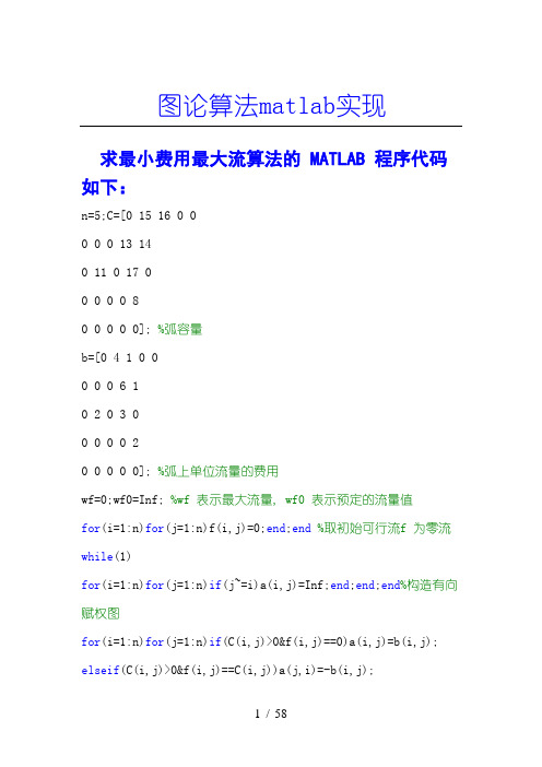
图论算法matlab实现求最小费用最大流算法的 MATLAB 程序代码如下:n=5;C=[0 15 16 0 00 0 0 13 140 11 0 17 00 0 0 0 80 0 0 0 0]; %弧容量b=[0 4 1 0 00 0 0 6 10 2 0 3 00 0 0 0 20 0 0 0 0]; %弧上单位流量的费用wf=0;wf0=Inf; %wf 表示最大流量, wf0 表示预定的流量值for(i=1:n)for(j=1:n)f(i,j)=0;end;end %取初始可行流f 为零流while(1)for(i=1:n)for(j=1:n)if(j~=i)a(i,j)=Inf;end;end;end%构造有向赋权图for(i=1:n)for(j=1:n)if(C(i,j)>0&f(i,j)==0)a(i,j)=b(i,j); elseif(C(i,j)>0&f(i,j)==C(i,j))a(j,i)=-b(i,j);elseif(C(i,j)>0)a(i,j)=b(i,j);a(j,i)=-b(i,j);end;end;end for(i=2:n)p(i)=Inf;s(i)=i;end %用Ford 算法求最短路, 赋初值for(k=1:n)pd=1; %求有向赋权图中vs 到vt 的最短路for(i=2:n)for(j=1:n)if(p(i)>p(j)+a(j,i))p(i)=p(j)+a(j,i);s( i)=j;pd=0;end;end;endif(pd)break;end;end %求最短路的Ford 算法结束if(p(n)==Inf)break;end %不存在vs 到vt 的最短路, 算法终止. 注意在求最小费用最大流时构造有向赋权图中不会含负权回路, 所以不会出现k=ndvt=Inf;t=n; %进入调整过程, dvt 表示调整量while(1) %计算调整量if(a(s(t),t)>0)dvtt=C(s(t),t)-f(s(t),t); %前向弧调整量elseif(a(s(t),t)<0)dvtt=f(t,s(t));end %后向弧调整量if(dvt>dvtt)dvt=dvtt;endif(s(t)==1)break;end %当t 的标号为vs 时, 终止计算调整量t=s(t);end %继续调整前一段弧上的流fpd=0;if(wf+dvt>=wf0)dvt=wf0-wf;pd=1;end%如果最大流量大于或等于预定的流量值t=n;while(1) %调整过程if(a(s(t),t)>0)f(s(t),t)=f(s(t),t)+dvt; %前向弧调整elseif(a(s(t),t)<0)f(t,s(t))=f(t,s(t))-dvt;end %后向弧调整if(s(t)==1)break;end %当t 的标号为vs 时, 终止调整过程t=s(t);endif(pd)break;end%如果最大流量达到预定的流量值wf=0; for(j=1:n)wf=wf+f(1,j);end;end %计算最大流量zwf=0;for(i=1:n)for(j=1:n)zwf=zwf+b(i,j)*f(i,j);end;end%计算最小费用f %显示最小费用最大流图 6-22wf %显示最小费用最大流量zwf %显示最小费用, 程序结束__Kruskal 避圈法:Kruskal 避圈法的MATLAB 程序代码如下:n=8;A=[0 2 8 1 0 0 0 02 0 6 0 1 0 0 08 6 0 7 5 1 2 01 0 7 0 0 0 9 00 1 5 0 0 3 0 80 0 1 0 3 0 4 60 0 2 9 0 4 0 30 0 0 0 8 6 3 0];k=1; %记录A中不同正数的个数for(i=1:n-1)for(j=i+1:n) %此循环是查找A中所有不同的正数if(A(i,j)>0)x(k)=A(i,j); %数组x 记录A中不同的正数kk=1; %临时变量for(s=1:k-1)if(x(k)==x(s))kk=0;break;end;end %排除相同的正数k=k+kk;end;end;endk=k-1 %显示A中所有不同正数的个数for(i=1:k-1)for(j=i+1:k) %将x 中不同的正数从小到大排序if(x(j)<x(i))xx=x(j);x(j)=x(i);x(i)=xx;end;end;endT(n,n)=0; %将矩阵T 中所有的元素赋值为0q=0; %记录加入到树T 中的边数for(s=1:k)if(q==n)break;end %获得最小生成树T, 算法终止for(i=1:n-1)for(j=i+1:n)if(A(i,j)==x(s))T(i,j)=x(s);T(j,i)=x(s); %加入边到树T 中TT=T; %临时记录Twhile(1)pd=1; %砍掉TT 中所有的树枝for(y=1:n)kk=0;for(z=1:n)if(TT(y,z)>0)kk=kk+1;zz=z;end;end %寻找TT 中的树枝if(kk==1)TT(y,zz)=0;TT(zz,y)=0;pd=0;end;end %砍掉TT 中的树枝if(pd)break;end;end %已砍掉了TT 中所有的树枝pd=0; %判断TT 中是否有圈for(y=1:n-1)for(z=y+1:n)if(TT(y,z)>0)pd=1;break;end;end;end if(pd)T(i,j)=0;T(j,i)=0; %假如TT 中有圈else q=q+1;end;end;end;end;endT %显示近似最小生成树T, 程序结束用Warshall-Floyd 算法求任意两点间的最短路.n=8;A=[0 2 8 1 Inf Inf Inf Inf2 0 6 Inf 1 Inf Inf Inf8 6 0 7 5 1 2 Inf1 Inf 7 0 Inf Inf 9 Inf Inf 1 5 Inf 0 3 Inf 8 Inf Inf 1 Inf 3 0 4 6Inf Inf 2 9 Inf 4 0 3Inf Inf Inf Inf 8 6 3 0]; % MATLAB 中, Inf 表示∞D=A; %赋初值for(i=1:n)for(j=1:n)R(i,j)=j;end;end %赋路径初值for(k=1:n)for(i=1:n)for(j=1:n)if(D(i,k)+D(k,j)<D(i,j))D(i,j )=D(i,k)+D(k,j); %更新dijR(i,j)=k;end;end;end %更新rijk %显示迭代步数D %显示每步迭代后的路长R %显示每步迭代后的路径pd=0;for i=1:n %含有负权时if(D(i,i)<0)pd=1;break;end;end %存在一条含有顶点vi 的负回路if(pd)break;end %存在一条负回路, 终止程序end %程序结束利用 Ford--Fulkerson 标号法求最大流算法的MATLAB 程序代码如下:n=8;C=[0 5 4 3 0 0 0 00 0 0 0 5 3 0 00 0 0 0 0 3 2 00 0 0 0 0 0 2 00 0 0 0 0 0 0 40 0 0 0 0 0 0 30 0 0 0 0 0 0 50 0 0 0 0 0 0 0]; %弧容量for(i=1:n)for(j=1:n)f(i,j)=0;end;end %取初始可行流f 为零流for(i=1:n)No(i)=0;d(i)=0;end %No,d 记录标号图 6-19while(1)No(1)=n+1;d(1)=Inf; %给发点vs 标号while(1)pd=1; %标号过程for(i=1:n)if(No(i)) %选择一个已标号的点vifor(j=1:n)if(No(j)==0&f(i,j)<C(i,j)) %对于未给标号的点vj, 当vivj 为非饱和弧时No(j)=i;d(j)=C(i,j)-f(i,j);pd=0;if(d(j)>d(i))d(j)=d(i);endelseif(No(j)==0&f(j,i)>0) %对于未给标号的点vj, 当vjvi 为非零流弧时No(j)=-i;d(j)=f(j,i);pd=0;if(d(j)>d(i))d(j)=d(i);end;end;end;end;endif(No(n)|pd)break;end;end%若收点vt 得到标号或者无法标号, 终止标号过程if(pd)break;end %vt 未得到标号, f 已是最大流, 算法终止dvt=d(n);t=n; %进入调整过程, dvt 表示调整量while(1)if(No(t)>0)f(No(t),t)=f(No(t),t)+dvt; %前向弧调整elseif(No(t)<0)f(No(t),t)=f(No(t),t)-dvt;end %后向弧调整if(No(t)==1)for(i=1:n)No(i)=0;d(i)=0; end;break;end %当t 的标号为vs 时, 终止调整过程t=No(t);end;end; %继续调整前一段弧上的流fwf=0;for(j=1:n)wf=wf+f(1,j);end %计算最大流量f %显示最大流wf %显示最大流量No %显示标号, 由此可得最小割, 程序结束图论程序大全程序一:关联矩阵和邻接矩阵互换算法function W=incandadf(F,f)if f==0m=sum(sum(F))/2;n=size(F,1);W=zeros(n,m);k=1;for i=1:nfor j=i:nif F(i,j)~=0W(i,k)=1;W(j,k)=1;k=k+1;endendendelseif f==1m=size(F,2);n=size(F,1);W=zeros(n,n);for i=1:ma=find(F(:,i)~=0);W(a(1),a(2))=1;W(a(2),a(1))=1;endelsefprint('Please imput the right value of f');endW;程序二:可达矩阵算法function P=dgraf(A) n=size(A,1);P=A;for i=2:nP=P+A^i;endP(P~=0)=1;P;程序三:有向图关联矩阵和邻接矩阵互换算法function W=mattransf(F,f)if f==0m=sum(sum(F));n=size(F,1);W=zeros(n,m);k=1;for i=1:nfor j=i:nif F(i,j)~=0W(i,k)=1;W(j,k)=-1;k=k+1;endendendelseif f==1m=size(F,2);n=size(F,1);W=zeros(n,n);for i=1:ma=find(F(:,i)~=0);if F(a(1),i)==1W(a(1),a(2))=1;elseW(a(2),a(1))=1;endendelsefprint('Please imput the right value of f');endW;第二讲:最短路问题程序一:Dijkstra算法(计算两点间的最短路)function [l,z]=Dijkstra(W)n = size (W,1); for i = 1 :nl(i)=W(1,i);z(i)=0;endi=1;while i<=nfor j =1 :nif l(i)>l(j)+W(j,i)l(i)=l(j)+W(j,i);z(i)=j-1;if j<ii=j-1;endendendi=i+1;end程序二:floyd算法(计算任意两点间的最短距离)function [d,r]=floyd(a)n=size(a,1);d=a;for i=1:nfor j=1:nr(i,j)=j;endendr;for k=1:nfor i=1:nfor j=1:nif d(i,k)+d(k,j)<d(i,j)d(i,j)=d(i,k)+d(k,j);r(i,j)=r(i,k);endendendend程序三:n2short.m 计算指定两点间的最短距离function [P u]=n2short(W,k1,k2)n=length(W);U=W;m=1;while m<=nfor i=1:nfor j=1:nif U(i,j)>U(i,m)+U(m,j)U(i,j)=U(i,m)+U(m,j);endendendm=m+1;endu=U(k1,k2);P1=zeros(1,n);k=1;P1(k)=k2;V=ones(1,n)*inf;kk=k2;while kk~=k1for i=1:nV(1,i)=U(k1,kk)-W(i,kk);if V(1,i)==U(k1,i)P1(k+1)=i;kk=i;k=k+1;endendendk=1;wrow=find(P1~=0);for j=length(wrow):-1:1P(k)=P1(wrow(j));k=k+1;endP;程序四、n1short.m(计算某点到其它所有点的最短距离)function[Pm D]=n1short(W,k)n=size(W,1);D=zeros(1,n);for i=1:n[P d]=n2short(W,k,i);Pm{i}=P;D(i)=d;end程序五:pass2short.m(计算经过某两点的最短距离)function [P d]=pass2short(W,k1,k2,t1,t2)[p1 d1]=n2short(W,k1,t1);[p2 d2]=n2short(W,t1,t2);[p3 d3]=n2short(W,t2,k2);dt1=d1+d2+d3;[p4 d4]=n2short(W,k1,t2);[p5 d5]=n2short(W,t2,t1);[p6 d6]=n2short(W,t1,k2);dt2=d4+d5+d6;if dt1<dt2d=dt1;P=[p1 p2(2:length(p2)) p3(2:length(p3))];elsed=dt1;p=[p4 p5(2:length(p5)) p6(2:length(p6))];endP;d;第三讲:最小生成树程序一:最小生成树的Kruskal算法function [T c]=krusf(d,flag)if nargin==1n=size(d,2);m=sum(sum(d~=0))/2;b=zeros(3,m);k=1;for i=1:nfor j=(i+1):nif d(i,j)~=0b(1,k)=i;b(2,k)=j;b(3,k)=d(i,j);k=k+1;endendendelseb=d;endn=max(max(b(1:2,:)));m=size(b,2);[B,i]=sortrows(b',3);B=B';c=0;T=[];k=1;t=1:n;for i=1:mif t(B(1,i))~=t(B(2,i))T(1:2,k)=B(1:2,i);c=c+B(3,i);k=k+1;tmin=min(t(B(1,i)),t(B(2,i)));tmax=max(t(B(1,i)),t(B(2,i)));for j=1:nif t(j)==tmaxt(j)=tmin;endendendif k==nbreak;endendT;c;程序二:最小生成树的Prim算法function [T c]=Primf(a)l=length(a);a(a==0)=inf;k=1:l;listV(k)=0;listV(1)=1;e=1;while (e<l)min=inf;for i=1:lif listV(i)==1for j=1:lif listV(j)==0 & min>a(i,j)min=a(i,j);b=a(i,j);s=i;d=j;endendendendlistV(d)=1;distance(e)=b;source(e)=s;destination(e)=d;e=e+1;endT=[source;destination]; for g=1:e-1c(g)=a(T(1,g),T(2,g));endc;另外两种程序最小生成树程序1(prim 算法构造最小生成树)a=[inf 50 60 inf inf inf inf;50 inf inf 65 40 inf inf;60 inf inf 52 inf inf 45;...inf 65 52 inf 50 30 42;inf 40 inf 50 inf 70 inf;inf inf inf 30 70 inf inf;...inf inf 45 42 inf inf inf];result=[];p=1;tb=2:length(a);while length(result)~=length(a)-1temp=a(p,tb);temp=temp(:);d=min(temp);[jb,kb]=find(a(p,tb)==d);j=p(jb(1));k=tb(kb(1));result=[result,[j;k;d]];p=[p,k];tb(find(tb==k))=[];endresult最小生成树程序2(Kruskal 算法构造最小生成树)clc;clear;a(1,2)=50; a(1,3)=60; a(2,4)=65; a(2,5)=40;a(3,4)=52;a(3,7)=45; a(4,5)=50; a(4,6)=30;a(4,7)=42; a(5,6)=70;[i,j,b]=find(a);data=[i';j';b'];index=data(1:2,:);loop=max(size(a))-1;result=[];while length(result)<looptemp=min(data(3,:));flag=find(data(3,:)==temp);flag=flag(1);v1=data(1,flag);v2=data(2,flag);if index(1,flag)~=index(2,flag)result=[result,data(:,flag)];endindex(find(index==v2))=v1;data(:,flag)=[];index(:,flag)=[];endresult第四讲:Euler图和Hamilton图程序一:Fleury算法(在一个Euler图中找出Euler环游)注:包括三个文件;fleuf1.m, edf.m, flecvexf.mfunction [T c]=fleuf1(d)%注:必须保证是Euler环游,否则输出T=0,c=0 n=length(d);b=d;b(b==inf)=0;b(b~=0)=1;m=0;a=sum(b);eds=sum(a)/2;ed=zeros(2,eds);vexs=zeros(1,eds+1);matr=b;for i=1:nif mod(a(i),2)==1m=m+1;endendif m~=0fprintf('there is not exit Euler path.\n')T=0;c=0;endif m==0vet=1;flag=0;t1=find(matr(vet,:)==1);for ii=1:length(t1)ed(:,1)=[vet,t1(ii)];vexs(1,1)=vet;vexs(1,2)=t1(ii);matr(vexs(1,2),vexs(1,1))=0;flagg=1;tem=1;while flagg[flagg ed]=edf(matr,eds,vexs,ed,tem); tem=tem+1;if ed(1,eds)~=0 & ed(2,eds)~=0T=ed;T(2,eds)=1;c=0;for g=1:edsc=c+d(T(1,g),T(2,g));endflagg=0;break;endendendendfunction[flag ed]=edf(matr,eds,vexs,ed,tem)flag=1;for i=2:eds[dvex f]=flecvexf(matr,i,vexs,eds,ed,tem);if f==1flag=0;break;endif dvex~=0ed(:,i)=[vexs(1,i) dvex];vexs(1,i+1)=dvex;matr(vexs(1,i+1),vexs(1,i))=0;elsebreak;endendfunction [dvex f]=flecvexf(matr,i,vexs,eds,ed,temp) f=0;edd=find(matr(vexs(1,i),:)==1);dvex=0;dvex1=[];ded=[];if length(edd)==1dvex=edd;elsedd=1;dd1=0;kkk=0;for kk=1:length(edd)m1=find(vexs==edd(kk));if sum(m1)==0dvex1(dd)=edd(kk);dd=dd+1;dd1=1;elsekkk=kkk+1;endendif kkk==length(edd)tem=vexs(1,i)*ones(1,kkk);edd1=[tem;edd];for l1=1:kkklt=0;ddd=1;for l2=1:edsif edd1(1:2,l1)==ed(1:2,l2)lt=lt+1;endendif lt==0ded(ddd)=edd(l1); ddd=ddd+1;endendendif temp<=length(dvex1)dvex=dvex1(temp);elseif temp>length(dvex1) & temp<=length(ded)dvex=ded(temp);elsef=1;endend程序二:Hamilton改良圈算法(找出比较好的Hamilton路)function [C d1]= hamiltonglf(v)%d表示权值矩阵%C表示算法最终找到的Hamilton圈。
最短路径 dijkstra算法的matlab代码实现
最短路径dijkstra算法的matlab代码实现如何用Matlab实现Dijkstra算法求解最短路径问题?Dijkstra算法是一种用于计算图中的最短路径的经典算法。
该算法以一个起始节点为基础,通过不断更新节点到其他节点的最短距离,直到找到最短路径为止。
本文将一步一步地回答如何使用Matlab实现Dijkstra算法,以及如何在Matlab中构建图并求解最短路径。
第一步:构建图Dijkstra算法是基于图的算法,因此我们首先需要在Matlab中构建一个图。
图可以用邻接矩阵或邻接表等方式表示。
这里我们选择使用邻接矩阵来表示图。
在Matlab中,可以使用矩阵来表示邻接矩阵。
假设我们的图有n个节点,我们可以创建一个n×n的矩阵来表示图的邻接矩阵。
如果节点i和节点j 之间有一条边,则将邻接矩阵中的第i行第j列的元素设置为边的权重,如果没有边相连,则将元素设置为一个较大的值(例如无穷大)表示不可达。
现在,我们可以开始构建邻接矩阵。
这里以一个具体的例子来说明。
假设我们有一个包含6个节点的无向图,如下所示:0 1 2 3 4 5-0 0 4 3 0 0 01 4 0 1 4 0 02 3 1 0 2 1 03 04 2 0 3 24 0 0 1 3 0 25 0 0 0 2 2 0在Matlab中,可以将邻接矩阵表示为一个n×n的矩阵。
在这个例子中,我们可以这样定义邻接矩阵:G = [0 4 3 0 0 0;4 0 1 4 0 0;3 1 0 2 1 0;0 4 2 0 3 2;0 0 1 3 0 2;0 0 0 2 2 0];第二步:实现Dijkstra算法在Matlab中,我们可以使用一些循环和条件语句来实现Dijkstra算法。
下面是一个基本的Dijkstra算法的实现流程:1. 创建一个数组dist,用于存储从起始节点到其他节点的最短距离。
初始时,将起始节点到自身的距离设置为0,其他节点的距离设置为无穷大。
MATLAB解决最短路径问题代码
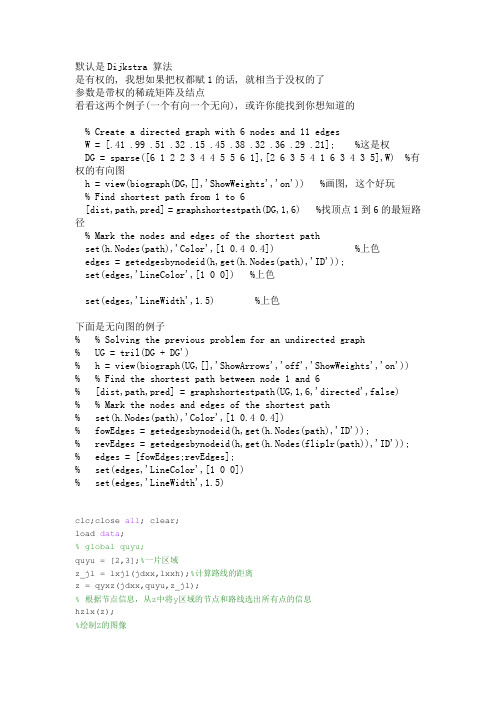
默认是Dijkstra 算法是有权的, 我想如果把权都赋1的话, 就相当于没权的了参数是带权的稀疏矩阵及结点看看这两个例子(一个有向一个无向), 或许你能找到你想知道的% Create a directed graph with 6 nodes and 11 edgesW = [.41 .99 .51 .32 .15 .45 .38 .32 .36 .29 .21]; %这是权DG = sparse([6 1 2 2 3 4 4 5 5 6 1],[2 6 3 5 4 1 6 3 4 3 5],W) %有权的有向图h = view(biograph(DG,[],'ShowWeights','on')) %画图, 这个好玩% Find shortest path from 1 to 6[dist,path,pred] = graphshortestpath(DG,1,6) %找顶点1到6的最短路径% Mark the nodes and edges of the shortest pathset(h.Nodes(path),'Color',[1 0.4 0.4]) %上色edges = getedgesbynodeid(h,get(h.Nodes(path),'ID'));set(edges,'LineColor',[1 0 0]) %上色set(edges,'LineWidth',1.5) %上色下面是无向图的例子% % Solving the previous problem for an undirected graph% UG = tril(DG + DG')% h = view(biograph(UG,[],'ShowArrows','off','ShowWeights','on')) % % Find the shortest path between node 1 and 6% [dist,path,pred] = graphshortestpath(UG,1,6,'directed',false)% % Mark the nodes and edges of the shortest path% set(h.Nodes(path),'Color',[1 0.4 0.4])% fowEdges = getedgesbynodeid(h,get(h.Nodes(path),'ID'));% revEdges = getedgesbynodeid(h,get(h.Nodes(fliplr(path)),'ID')); % edges = [fowEdges;revEdges];% set(edges,'LineColor',[1 0 0])% set(edges,'LineWidth',1.5)clc;close all; clear;load data;% global quyu;quyu = [2,3];%一片区域z_jl = lxjl(jdxx,lxxh);%计算路线的距离z = qyxz(jdxx,quyu,z_jl);% 根据节点信息,从z中将y区域的节点和路线选出所有点的信息hzlx(z);%绘制Z的图像[qypt, nqypt] = ptxzm(xjpt,quyu);changdu = length(bhxz(jdxx,1:6));%选出x中y区的标号,只是分区域,求长度并绘制它tt = z(:,[1,2,end])';k = min(min(tt(1:2,:)));%求两次最小值t = tt(1:2,:) ;xsjz = sparse(t(2,:),t(1,:),tt(3,:),changdu,changdu);%产生稀疏矩阵[dist, path, pred] = zdljxz(xsjz, qypt, k );%三个原包矩阵通过zdljxz计算得到最短路径hold onfor j = 1:nqyptcolors = rand(1,3);%产生随机数并用颜色标记hzptxc(path{j},jdxx,colors)endhold offaxis equal%把坐标轴单位设为相等zjd = jdfgd( path, quyu);function z = lxjl(x, y)%计算路线的距离[m n] = size(y);for i = 1:myy(i,1:2) = x(y(i,1),2:3);yy(i,3:4) = x(y(i,2),2:3);endz = sqrt((yy(:,3) - yy(:,1)).^2 + (yy(:,2) - yy(:,4)).^2);y = sort(y');y = y';z = [y yy z];z = sortrows(z);function [z lz] = ptxz(xjpt,y)pt = xjpt(:,2);wei = ismember(xjpt(:,1),y);z = pt(wei);lz = length(z);unction hzptxc(path,jdxx,colors)n = length(path);% hold onfor i = 1:nhzptjd(jdxx, path{i},colors)end% hold offunction hzptjd(jdxx,x,colors)% m = length(x);% x = x';hold onplot(jdxx(x,2),jdxx(x,3),'o','LineStyle' ,'-' ,...'Color',colors,'MarkerEdgeColor',colors)plot(jdxx(x(1),2),jdxx(x(1),3),'*','MarkerFaceColor',colors)hold offfunction hzlx(x)%绘制x的图像[m n] = size(x);hold onfor i = 1:mplot([x(i,3) x(i,5)],[x(i,4) x(i,6)],'k:')endhold offfunction z = bhxz(x,y)%选出x中y区的标号,只是分区域xzq = x(:,4);xzr = ismember(xzq,y);z = x(xzr,:);z = z(:,1);。
中国海洋大学本科生课程大纲

中国海洋大学本科生课程大纲课程名称数学实验Mathematics Experiments课程代码 0751********课程属性 工作技能 课时/学分64/2课程性质 必修 实践学时 64 责任教师 施心慧 课外学时 0 课程属性:公共基础/通识教育/学科基础/专业知识/工作技能,课程性质:必修、选修一、 课程介绍1.课程描述:数学实验是由于计算机技术和科学计算软件的迅猛发展应运而生的一门较新的数学课程,它改变了数学只靠纸和笔的传统形象,将实验的手段引入到数学的学习和研究中。
本课程为大学二年级数学院的学生开设。
它不是讲授新的数学知识,而是让学生利用已有的数学知识去解决一些经简化的实际问题。
大多数实验的一般过程是:对于给出的实际问题,建立数学模型、选择适当的数学方法、用科学计算软件MATLAB编程计算、对运算结果进行分析、给出结论。
本课程以MATLAB软件为主要的实验工具,采用以学生动手动脑为主,教师讲授和点评、小组讨论、报告为辅的教学方式。
通过本课程的学习,学生用数学解决实际问题的意识和能力可以得到强化和提高,更切实地体会到数学的用处,增加学习兴趣,提高创造力。
2.设计思路:本课程旨在训练用数学解决实际问题的能力。
实验内容的选取是基于学生具备MATLAB语言的初步编程能力、并学习了数学分析、高等代数、解析几何、运筹学基础(初步)、数学实验基础、常微分方程、数值分析或计算方法、概率论等数学课程的基础之上。
课程共分七个基础实验和一个综合实验依次进行。
七个基础实验是:MATLAB 基础知识复习、常微分方程(组)、数据建模——插值与拟合、古典密码学、图与网络- 1 -优化、动态规划、遗传算法。
基础实验涉及的数学内容较为单一、数学模型和求解方法较简单,是对“用数学”能力的基本训练。
综合实验以三人为一组进行,所涉及到的数学知识范围更广,建模和求解的难度更大。
综合实验的题目可以小组自拟或在任课教师拟定的题目中选择。
加权聚类系数和加权平均路径长度matlab代码

加权聚类系数和加权平均路径长度matlab代码加权聚类系数和加权平均路径长度是图论中一对重要的指标,用于评价网络图中节点之间的连接密度和通信效率。
在本文中,我将重点介绍加权聚类系数和加权平均路径长度的概念,并提供相应的Matlab代码来计算这些指标。
1. 加权聚类系数加权聚类系数是一种度量网络图中节点局部连接密度的指标。
对于一个节点而言,它的聚类系数定义为该节点的邻居节点之间实际存在的边数与可能存在的边数的比值。
在加权网络图中,我们需要考虑边的权重。
对于给定的节点i,其邻居节点集合定义为Ni,该节点的聚类系数Ci可以通过以下步骤计算得到:1. 对于节点i的每对邻居节点j和k,计算其边的权重wij和wik。
2. 对于每对邻居节点j和k,计算其边的权重的乘积相加,即sum =Σ(wij * wik)。
3. 计算节点i的邻居节点之间可能的边数,即possible_edges = (|Ni| * (|Ni| - 1)) / 2。
4. 计算节点i的加权聚类系数Ci = 2 * sum / possible_edges。
下面是使用Matlab实现计算加权聚类系数的代码:```matlabfunction weighted_clustering_coefficient =compute_weighted_clustering_coefficient(adjacency_matrix) num_nodes = size(adjacency_matrix, 1);weighted_clustering_coefficient = zeros(num_nodes, 1);for i = 1:num_nodesneighbors = find(adjacency_matrix(i, :) > 0);num_neighbors = length(neighbors);if num_neighbors >= 2weights = adjacency_matrix(i, neighbors);weighted_sum = 0;for j = 1:num_neighbors-1for k = j+1:num_neighborsweighted_sum = weighted_sum + (weights(j) * weights(k));endendpossible_edges = (num_neighbors * (num_neighbors - 1)) / 2;weighted_clustering_coefficient(i) = 2 * weighted_sum / possible_edges;endendend```在上述代码中,我们首先根据给定的邻接矩阵的大小确定节点数量。
- 1、下载文档前请自行甄别文档内容的完整性,平台不提供额外的编辑、内容补充、找答案等附加服务。
- 2、"仅部分预览"的文档,不可在线预览部分如存在完整性等问题,可反馈申请退款(可完整预览的文档不适用该条件!)。
- 3、如文档侵犯您的权益,请联系客服反馈,我们会尽快为您处理(人工客服工作时间:9:00-18:30)。
学号:
课程设计
题目Dijkstra算法的MATLAB实现
学院信息工程学院
专业通信工程
班级
姓名
指导教师
2012 年 1 月9 日
课程设计任务书
学生姓名:专业班级:通信 0901班
指导教师:工作单位:信息工程学院
题目: Dijkstra算法的MATLAB实现
初始条件:
(1)MATLAB应用软件的基本知识以及基本操作技能
(2)高等数学、线性代数等基础数学中的运算知识
(3)数据结构里面关于Dijkstra算法的基本原理和思想
要求完成的主要任务:
必做题:采用MATLAB选用适当的函数或矩阵进行如下计算
(1)极限的计算、微分的计算、积分的计算、级数的计算、求解代数方程、求解常微分方程;
(2)矩阵的最大值、最小值、均值、方差、转置、逆、行列式、特征值的计算、矩阵的相乘、右除、左除、幂运算;
(3)多项式加减乘除运算、多项式求导、求根和求值运算、多项式的部分分式展开、多项式的拟合、插值运算。
选做题:Dijkstra算法的MATLAB实现
时间安排:
第一周,安排任务地点:鉴主17楼实验室
第1-17,周仿真设计地点:鉴主13楼计算机实验室
第18周,完成答辩,提交报告地点:鉴主17楼实验室
指导教师签名:年月日
系主任(或责任教师)签名:年月
目录
摘要 (I)
Abstract (II)
1 MATLAB的基本运算 0
1.1 基础微积分计算 0
1.1.1 极限的基本运算 0
1.1.2 微分的计算 0
1.1.3 积分的计算 (1)
1.1.4 级数的运算 (1)
1.1.5 求解代数微分方程 (1)
1.1.6 求解常微分方程 (2)
1.2 矩阵的基本运算 (2)
1.2.1 矩阵的最大最小值 (2)
1.2.2 矩阵的均值方差 (3)
1.2.3 矩阵的转置和逆 (3)
1.2.4 矩阵的行列式 (3)
1.2.5 矩阵特征值的计算 (3)
1.2.6 矩阵的相乘 (4)
1.2.7 矩阵的右除和左除 (4)
1.2.8 矩阵的幂运算 (4)
1.3 多项式的基本运算 (4)
1.3.1 多项式的四则运算 (4)
1.3.2 多项式的求导、求根、求值运算 (5)
1.3.3 多项式的部分分式展开 (5)
1.3.4 多项式的拟合 (5)
1.3.5 多项式的插值运算 (6)
2关于Dijkstra的问题描述 (6)
2.1问题的提出 (6)
2.2 Dijkstra算法的算法思想 (7)
2.3 Dijkstra算法的算法原理 (7)
3 Dijkstra算法的设计分析 (8)
3.1 Dijkstra算法部分的设计分析 (8)
3.2 程序主体的设计分析 (9)
4程序源代码与算法思想 (10)
4.1 文件isIn.m的源代码 (10)
4.2 文件default_dat.m的源代码 (11)
4.3 文件input_dat.m的源代码 (11)
4.4 文件menu.m的源代码 (11)
4.5 文件dijkstra.m的源代码 (13)
5 测试报告 (16)
6 心得体会 (17)
7 参考文献 (18)。