
多旅行商问题的matlab程序
多旅行商问题的m a t l a b程序Document serial number【NL89WT-NY98YT-NC8CB-NNUUT-NUT108】%多旅行商问题的m a t l a b程序function varargout =mtspf_ga(xy,dmat,salesmen,min_tour,pop_size,num_iter,show_prog,show_r es)% MTSPF_GA Fixed Multiple Traveling Salesmen Problem (M-TSP) Genetic Algorithm (GA)% Finds a (near) optimal solution to a variation of the M-TSP by setting% up a GA to search for the shortest route (least distance needed for% each salesman to travel from the start location to individual cities% and back to the original starting place)%% Summary:% 1. Each salesman starts at the first point, and ends at thefirst% point, but travels to a unique set of cities in between% 2. Except for the first, each city is visited by exactly one salesman%% Note: The Fixed Start/End location is taken to be the first XY point%% Input:% XY (float) is an Nx2 matrix of city locations, where N is the number of cities% DMAT (float) is an NxN matrix of city-to-city distances or costs% SALESMEN (scalar integer) is the number of salesmen to visit the cities% MIN_TOUR (scalar integer) is the minimum tour length for any of the% salesmen, NOT including the start/end point% POP_SIZE (scalar integer) is the size of the population (should be divisible by 8)% NUM_ITER (scalar integer) is the number of desired iterations for the algorithm to run% SHOW_PROG (scalar logical) shows the GA progress if true% SHOW_RES (scalar logical) shows the GA results if true%% Output:% OPT_RTE (integer array) is the best route found by the algorithm% OPT_BRK (integer array) is the list of route break points (these specify the indices% into the route used to obtain the individual salesman routes)% MIN_DIST (scalar float) is the total distance traveled by the salesmen%% Route/Breakpoint Details:% If there are 10 cities and 3 salesmen, a possible route/break% combination might be: rte = [5 6 9 4 2 8 10 3 7], brks = [3 7] % Taken together, these represent the solution [1 5 6 9 1][1 4 2 8 1][1 10 3 7 1],% which designates the routes for the 3 salesmen as follows:% . Salesman 1 travels from city 1 to 5 to 6 to 9 and back to 1% . Salesman 2 travels from city 1 to 4 to 2 to 8 and back to 1% . Salesman 3 travels from city 1 to 10 to 3 to 7 and back to 1%% 2D Example:% n = 35;% xy = 10*rand(n,2);% salesmen = 5;% min_tour = 3;% pop_size = 80;% num_iter = 5e3;% a = meshgrid(1:n);% dmat = reshape(sqrt(sum((xy(a,:)-xy(a',:)).^2,2)),n,n);% [opt_rte,opt_brk,min_dist] =mtspf_ga(xy,dmat,salesmen,min_tour, ...% pop_size,num_iter,1,1);%% 3D Example:% n = 35;% xyz = 10*rand(n,3);% salesmen = 5;% min_tour = 3;% pop_size = 80;% num_iter = 5e3;% a = meshgrid(1:n);% dmat = reshape(sqrt(sum((xyz(a,:)-xyz(a',:)).^2,2)),n,n);% [opt_rte,opt_brk,min_dist] =mtspf_ga(xyz,dmat,salesmen,min_tour, ...% pop_size,num_iter,1,1);%% See also: mtsp_ga, mtspo_ga, mtspof_ga, mtspofs_ga, mtspv_ga, distmat%% Author: Joseph Kirk% Email% Release:% Release Date: 6/2/09% Process Inputs and Initialize Defaultsnargs = 8;for k = nargin:nargs-1switch kcase 0xy = 10*rand(40,2);case 1N = size(xy,1);a = meshgrid(1:N);dmat = reshape(sqrt(sum((xy(a,:)-xy(a',:)).^2,2)),N,N); case 2salesmen = 5;case 3min_tour = 2;case 4pop_size = 80;case 5num_iter = 5e3;case 6show_prog = 1;case 7show_res = 1;otherwiseendend% Verify Inputs[N,dims] = size(xy);[nr,nc] = size(dmat);if N ~= nr || N ~= ncerror('Invalid XY or DMAT inputs!')endn = N - 1; % Separate Start/End City% Sanity Checkssalesmen = max(1,min(n,round(real(salesmen(1)))));min_tour = max(1,min(floor(n/salesmen),round(real(min_tour(1))))); pop_size = max(8,8*ceil(pop_size(1)/8));num_iter = max(1,round(real(num_iter(1))));show_prog = logical(show_prog(1));show_res = logical(show_res(1));% Initializations for Route Break Point Selectionnum_brks = salesmen-1;dof = n - min_tour*salesmen; % degrees of freedomaddto = ones(1,dof+1);for k = 2:num_brksaddto = cumsum(addto);endcum_prob = cumsum(addto)/sum(addto);% Initialize the Populationspop_rte = zeros(pop_size,n); % population of routespop_brk = zeros(pop_size,num_brks); % population of breaksfor k = 1:pop_sizepop_rte(k,:) = randperm(n)+1;pop_brk(k,:) = randbreaks();end% Select the Colors for the Plotted Routesclr = [1 0 0; 0 0 1; 0 1; 0 1 0; 1 0];if salesmen > 5clr = hsv(salesmen);end% Run the GAglobal_min = Inf;total_dist = zeros(1,pop_size);dist_history = zeros(1,num_iter);tmp_pop_rte = zeros(8,n);tmp_pop_brk = zeros(8,num_brks);new_pop_rte = zeros(pop_size,n);new_pop_brk = zeros(pop_size,num_brks);if show_progpfig = figure('Name','MTSPF_GA | Current BestSolution','Numbertitle','off');endfor iter = 1:num_iter% Evaluate Members of the Populationfor p = 1:pop_sized = 0;p_rte = pop_rte(p,:);p_brk = pop_brk(p,:);rng = [[1 p_brk+1];[p_brk n]]';for s = 1:salesmend = d + dmat(1,p_rte(rng(s,1))); % Add Start Distancefor k = rng(s,1):rng(s,2)-1d = d + dmat(p_rte(k),p_rte(k+1));endd = d + dmat(p_rte(rng(s,2)),1); % Add End Distanceendtotal_dist(p) = d;end% Find the Best Route in the Population[min_dist,index] = min(total_dist);dist_history(iter) = min_dist;if min_dist < global_minglobal_min = min_dist;opt_rte = pop_rte(index,:);opt_brk = pop_brk(index,:);rng = [[1 opt_brk+1];[opt_brk n]]';if show_prog% Plot the Best Routefigure(pfig);for s = 1:salesmenrte = [1 opt_rte(rng(s,1):rng(s,2)) 1];if dims == 3, plot3(xy(rte,1),xy(rte,2),xy(rte,3),'.-','Color',clr(s,:));else plot(xy(rte,1),xy(rte,2),'.-','Color',clr(s,:)); endtitle(sprintf('Total Distance = %, Iteration= %d',min_dist,iter));hold onendif dims == 3, plot3(xy(1,1),xy(1,2),xy(1,3),'ko');else plot(xy(1,1),xy(1,2),'ko'); endhold offendend% Genetic Algorithm Operatorsrand_grouping = randperm(pop_size);for p = 8:8:pop_sizertes = pop_rte(rand_grouping(p-7:p),:);brks = pop_brk(rand_grouping(p-7:p),:);dists = total_dist(rand_grouping(p-7:p));[ignore,idx] = min(dists);best_of_8_rte = rtes(idx,:);best_of_8_brk = brks(idx,:);rte_ins_pts = sort(ceil(n*rand(1,2)));I = rte_ins_pts(1);J = rte_ins_pts(2);for k = 1:8 % Generate New Solutionstmp_pop_rte(k,:) = best_of_8_rte;tmp_pop_brk(k,:) = best_of_8_brk;switch kcase 2 % Fliptmp_pop_rte(k,I:J) = fliplr(tmp_pop_rte(k,I:J)); case 3 % Swaptmp_pop_rte(k,[I J]) = tmp_pop_rte(k,[J I]);case 4 % Slidetmp_pop_rte(k,I:J) = tmp_pop_rte(k,[I+1:J I]); case 5 % Modify Breakstmp_pop_brk(k,:) = randbreaks();case 6 % Flip, Modify Breakstmp_pop_rte(k,I:J) = fliplr(tmp_pop_rte(k,I:J)); tmp_pop_brk(k,:) = randbreaks();case 7 % Swap, Modify Breakstmp_pop_rte(k,[I J]) = tmp_pop_rte(k,[J I]);tmp_pop_brk(k,:) = randbreaks();case 8 % Slide, Modify Breakstmp_pop_rte(k,I:J) = tmp_pop_rte(k,[I+1:J I]); tmp_pop_brk(k,:) = randbreaks();otherwise % Do Nothingendendnew_pop_rte(p-7:p,:) = tmp_pop_rte;new_pop_brk(p-7:p,:) = tmp_pop_brk;endpop_rte = new_pop_rte;pop_brk = new_pop_brk;endif show_res% Plotsfigure('Name','MTSPF_GA | Results','Numbertitle','off');subplot(2,2,1);if dims == 3, plot3(xy(:,1),xy(:,2),xy(:,3),'k.');else plot(xy(:,1),xy(:,2),'k.'); endtitle('City Locations');subplot(2,2,2);imagesc(dmat([1 opt_rte],[1 opt_rte]));title('Distance Matrix');subplot(2,2,3);rng = [[1 opt_brk+1];[opt_brk n]]';for s = 1:salesmenrte = [1 opt_rte(rng(s,1):rng(s,2)) 1];if dims == 3, plot3(xy(rte,1),xy(rte,2),xy(rte,3),'.-','Color',clr(s,:));else plot(xy(rte,1),xy(rte,2),'.-','Color',clr(s,:)); endtitle(sprintf('Total Distance = %',min_dist));hold on;endif dims == 3, plot3(xy(1,1),xy(1,2),xy(1,3),'ko');else plot(xy(1,1),xy(1,2),'ko'); endsubplot(2,2,4);plot(dist_history,'b','LineWidth',2);title('Best Solution History');set(gca,'XLim',[0 num_iter+1],'YLim',[0 *max([1 dist_history])]); end% Return Outputsif nargoutvarargout{1} = opt_rte;varargout{2} = opt_brk;varargout{3} = min_dist;end% Generate Random Set of Break Pointsfunction breaks = randbreaks()if min_tour == 1 % No Constraints on Breakstmp_brks = randperm(n-1);breaks = sort(tmp_brks(1:num_brks));else % Force Breaks to be at Least the Minimum Tour Lengthnum_adjust = find(rand < cum_prob,1)-1;spaces = ceil(num_brks*rand(1,num_adjust));adjust = zeros(1,num_brks);for kk = 1:num_brksadjust(kk) = sum(spaces == kk);endbreaks = min_tour*(1:num_brks) + cumsum(adjust); endendend。
gurobi多目标问题matlab

Gurobi多目标问题在Matlab中的解决一、Gurobi简介Gurobi是一款强大的商业数学建模工具,广泛应用于优化领域。
它提供了多种优化算法,能够高效地解决线性规划、整数规划、二次规划等各种优化问题。
在实际工程和科学研究中,经常遇到多目标优化问题,即需要同时优化多个目标函数。
本文将介绍如何使用Gurobi在Matlab中解决多目标优化问题。
二、多目标优化问题的定义在多目标优化问题中,我们需要最小化或最大化多个目标函数,而且这些目标函数之间往往存在相互矛盾的关系。
在生产计划中,一个目标函数可能是最大化产量,另一个目标函数可能是最小化成本。
在实际应用中,我们需要找到一组可行的解,使得所有目标函数都达到一个较好的平衡。
三、Gurobi在Matlab中的调用在Matlab中调用Gurobi需要先安装Gurobi的Matlab接口。
安装完成后,我们可以在Matlab命令窗口中输入命令"gurobi"来验证是否成功安装。
接下来,我们需要在Matlab中编写代码,定义优化问题的目标函数、约束条件和变量类型。
在定义目标函数时,我们需要考虑多个目标函数之间的相关性,以及它们之间的权重关系。
在定义约束条件和变量类型时,我们需要考虑多目标函数之间可能存在的约束条件和变量之间的相互制约关系。
四、多目标优化问题的解决方法Gurobi提供了多种解决多目标优化问题的方法,包括加权法、约束法和Pareto最优解法等。
在加权法中,我们将多个目标函数进行线性组合,并引入权重因子来平衡各个目标函数之间的重要性。
在约束法中,我们将多个目标函数作为多个约束条件,通过逐步添加约束条件来找到最优解。
在Pareto最优解法中,我们寻找一组可行解,使得没有其他可行解能比它在所有目标函数上都更好。
五、案例分析以生产计划为例,假设我们需要同时考虑最大化产量和最小化成本两个目标。
我们可以先使用加权法,通过调整权重因子来平衡这两个目标的重要性,找到一个较好的解。
旅行商问题matlab源代码

function [pTS,fmin]=grTravSale(C)% Function [pTS,fmin]=grTravSale(C) solve the nonsymmetrical% traveling salesman problem.% Input parameter:% C(n,n) - matrix of distances between cities,% maybe, nonsymmetrical;% n - number of cities.% Output parameters:% pTS(n) - the order of cities;% fmin - length of way.% Uses the reduction to integer LP-problem:% Look: Miller C.E., Tucker A. W., Zemlin R. A.% Integer Programming Formulation of Traveling Salesman Problems. % J.ACM, 1960, Vol.7, p. 326-329.% Needed other products: MIQP.M.% This software may be free downloaded from site:% http://control.ee.ethz.ch/~hybrid/miqp/% Author: Sergiy Iglin% e-mail: siglin@yandex.ru% personal page: http://iglin.exponenta.ru% ============= Input data validation ==================if nargin<1,error('There are no input data!')endif ~isnumeric(C),error('The array C must be numeric!')endif ~isreal(C),error('The array C must be real!')ends=size(C); % size of array Cif length(s)~=2,error('The array C must be 2D!')endif s(1)~=s(2),error('Matrix C must be square!')endif s(1)<3,error('Must be not less than 3 cities!')end% ============ Size of problem ====================n=s(1); % number of vertexesm=n*(n-1); % number of arrows% ============ Parameters of integer LP problem ========Aeq=[]; % for the matrix of the boundary equationsfor k1=1:n,z1=zeros(n);z1(k1,:)=1;z2=[z1;eye(n)];Aeq=[Aeq z2([1:2*n-1],setdiff([1:n],k1))];endAeq=[Aeq zeros(2*n-1,n-1)];A=[]; % for the matrix of the boundary inequationsfor k1=2:n,z1=[];for k2=1:n,z2=eye(n)*(n-1)*(k2==k1);z1=[z1 z2(setdiff([2:n],k1),setdiff([1:n],k2))];endz2=-eye(n);z2(:,k1)=z2(:,k1)+1;A=[A;[z1 z2(setdiff([2:n],k1),2:n)]];endbeq=ones(2*n-1,1); % the right parts of the boundary equations b=ones((n-1)*(n-2),1)*(n-2); % the right parts of the boundary inequationsC1=C'+diag(ones(1,n)*NaN);C2=C1(:);c=[C2(~isnan(C2));zeros(n-1,1)]; % the factors for objective functionvlb=[zeros(m,1);-inf*ones(n-1,1)]; % the lower boundsvub=[ones(m,1);inf*ones(n-1,1)]; % the upper boundsH=zeros(n^2-1); % Hessian% ============= We solve the MIQP problem ========== [xmin,fmin]=MIQP(H,c,A,b,Aeq,beq,[1:m],vlb,vub);% ============= We return the results ==============eik=round(xmin(1:m)); % the arrows of the waye1=[zeros(1,n-1);reshape(eik,n,n-1)];e2=[e1(:);0]; % we add zero to a diagonale3=(reshape(e2,n,n))'; % the matrix of the waypTS=[1 find(e3(1,:))]; % we build the waywhile pTS(end)>1, % we add the city to the waypTS=[pTS find(e3(pTS(end),:))];endreturn。
matlab 遗传算法求解多式联运问题

文章标题:使用Matlab遗传算法求解多式联运问题在现代工程和科学领域中,多式联运问题是一种重要的优化问题。
它涉及到多个运输任务的分配和路径规划,对于提高运输效率和降低成本具有重要意义。
而遗传算法作为一种基于生物进化原理的优化方法,被广泛应用于解决多式联运问题。
本文将基于Matlab评台,探讨如何使用遗传算法来求解多式联运问题,并分析其优劣势。
1. 多式联运问题的定义多式联运问题是指在给定一组供应点和一组需求点之间,寻找最佳的运输方案,使得总运输成本最小化的问题。
这涉及到从供应点到需求点的路径规划和货物分配,其中包括运输成本、运输时间、货物数量等因素。
2. 遗传算法在多式联运问题中的应用遗传算法作为一种启发式搜索算法,通过模拟自然选择和遗传机制来寻找最优解。
在解决多式联运问题时,可以将每条路径或货物分配方案编码成染色体,通过交叉、变异等遗传操作来搜索最优解。
在Matlab中,可以利用遗传算法工具箱来实现多式联运问题的求解。
需要定义适应度函数,即评价每个个体(路径或分配方案)的好坏程度。
通过遗传算法工具箱中的函数,设置种群大小、遗传代数、交叉概率、变异概率等参数,进行遗传算法的求解过程。
3. 优缺点分析遗传算法作为一种全局搜索算法,对于多式联运问题具有较好的鲁棒性和全局寻优能力。
它能够在复杂的问题空间中搜索到较优解,对于大规模问题也有较好的适应性。
但是,遗传算法也存在着收敛速度慢、参数敏感性高等缺点,需要在具体应用中综合考虑。
4. 个人观点在解决多式联运问题时,我认为遗传算法是一种有效的求解方法。
它能够在不确定和复杂的问题中找到较优解,对于实际应用具有较强的适应性。
但是在使用遗传算法时,需要注意参数的设置和适应度函数的定义,以确保算法能够有效地搜索最优解。
总结本文详细介绍了在Matlab评台上使用遗传算法求解多式联运问题的方法和思路。
遗传算法作为一种全局搜索算法,对于多式联运问题具有较好的适应性和鲁棒性。
TSP旅行商问题matlab代码

if n==50
city50=[31 32;32 39;40 30;37 69;27 68;37 52;38 46;31 62;30 48;21 47;25 55;16 57;
17 63;42 41;17 33;25 32;5 64;8 52;12 42;7 38;5 25; 10 77;45 35;42 57;32 22;
end
s=smnew; %产生了新的种群
[f,p]=objf(s,dislist); %计算新种群的适应度
%记录当前代最好和平均的适应度
[fmax,nmax]=max(f);
ymean(gn)=1000/mean(f);
ymax(gn)=1000/fmax;
end
seln(i)=j; %选中个体的序号
if i==2&&j==seln(i-1) %%若相同就再选一次
r=rand; %产生一个随机数
prand=p-r;
j=1;
while prand(j)<0
j=j+1;
ymean=zeros(gn,1);
ymax=zeros(gn,1);
xmax=zeros(inn,CityNum);
scnew=zeros(inn,CityNum);
smnew=zeros(inn,CityNum);
while gn<gnmax+1
for j=1:2:inn
seln=sel(p); %选择操作
zhi=logical(scro(1,1:chb2)==scro(1,i));
y=scro(2,zhi);
scro(1,i)=y;
运输多染色体遗传的多旅行商问题matlab程序代码

运输多染色体遗传的多旅行商问题matlab程序代码篇一:多染色体遗传的多旅行商问题(Multi-迁徙 Problem in Multi-染色体 Gene Expression System)是一个复杂的生物信息学问题,通常需要通过数学建模来解决。
在这个问题中,个体在生殖过程中需要从不同的地区携带不同的基因型进行迁徙,以期望得到最大的基因型多样性。
在多旅行商问题中,每个个体需要在不同的染色体上携带不同的基因型,并且每个染色体上的基因型数量不同。
此外,每个地区需要适应不同的环境,因此每个地区的基因型变异率也有所不同。
因此,每个个体携带的基因型组合必须适应这个地区的环境,并且尽可能地增加个体的基因型多样性。
为了解决这个问题,可以使用数学建模的方法,将多旅行商问题转化为一个优化问题。
在这个优化问题中,个体的基因型多样性可以通过最大化一个函数来确定。
这个函数通常是一个组合优化问题,需要考虑到每个地区适应不同的环境以及每个染色体上的基因型数量的影响。
下面是一个用MATLAB求解多旅行商问题的示例代码,该代码使用了遗传算法来优化基因型多样性:```matlab% 多旅行商问题示例代码% 假设有n个染色体,每个染色体上有多个基因型% 定义基因型组合优化问题的目标函数function z = objective(a, b, c)z = a * (1 - b) * (1 - c) - b * a * c - a * (1 - b) * (1 - c) - c *a *b - b *c * a - c * b * c;end% 定义遗传算法的类classdef Multi迁徙Prob < handleversion 3.0% 定义个体的构造函数function this = Multi迁徙Prob(n, m) this.n = n;this.m = m;% 初始化种群if this.n < 2this.p = [1 1; 1 1];elsethis.p = randperm(this.n);end% 初始化随机变异源this.s = rand(this.n, 1);% 初始化个体this.i = 0;this.j = 0;this.k = 0;% 定义状态转移函数function this.next_state = stateif this.i == this.j && this.k == 0state = this.p;elsestate = rand();endend% 定义适应函数function this.适应 =适应(state)% 计算适应度if this.n == 2适应度 = [0.5 * this.s(1) * this.s(2); 0.5 * this.s(1) * this.s(2)]; else适应度 = [适应度; 0];end% 计算适应度矩阵this.a = [state(1); state(2)];this.b = [适应度; 0];this.c = [适应度; 0];% 计算适应度向量this.a = 适应度 * this.a;this.b = 适应度 * this.b;this.c = 适应度 * this.c;end% 初始化遗传算法的主循环this.m = 1;this.p = this.s;this.i = 0;this.j = 0;this.k = 0;% 计算初始种群中个体的适应度this.a = [this.a; this.b; this.c]; this.p[this.i] = this.a;this.p[this.j] = this.a;this.p[this.k] = this.a;% 迭代种群中的个体for this.l = 1:this.m% 随机选择一个个体this.l = randperm(this.n);% 计算当前个体的适应度this.a = [this.a; this.b; this.c];this.p[this.i + 1] = this.a;this.p[this.j + 1] = this.a;this.p[this.k + 1] = this.a;% 计算当前个体的基因型this.i = this.i + 1;this.j = this.j + 1;this.k = this.k + 1;this.j = j;this.k = k;% 计算当前个体的适应度向量this.b = [适应度; this.s(j) * this.s(k)];this.c = [适应度; this.s(j) * this.s(k)]; end% 计算种群中个体的适应度this.a = [this.a; this.b; this.c];this.p = this.p + this.a;% 计算适应度矩阵this.a = 适应度 * this.a;this.b = 适应度 * this.b;this.c = 适应度 * this.c;% 计算种群中个体的基因型this.i = this.i + 1;this.j = this.j + 1;this.k = this.k + 1;this.j = j;this.k = k;% 计算种群中个体的适应度向量this.a = [适应度; this.s(j) * this.s(k)]; this.p = this.p + this.a;% 输出最终适应度this.a = [适应度; this.s(j) * this.s(k)];% 输出最终基因型多样性z = objective(this.p, this.a, this.b, this.c);endend```该代码使用遗传算法来解决多旅行商问题,通过优化个体的基因型多样性来实现最大的基因型多样性。
多旅行商问题的matlab程序
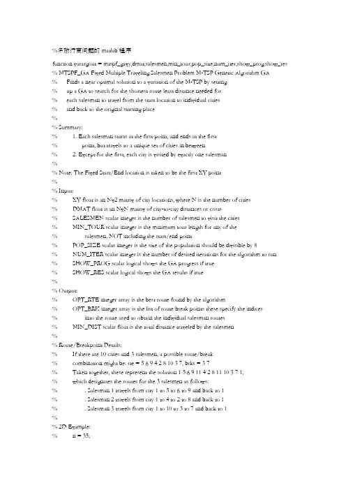
%多旅行商问题的matlab程序function varargout = mtspf_gaxy,dmat,salesmen,min_tour,pop_size,num_iter,show_prog,show_res % MTSPF_GA Fixed Multiple Traveling Salesmen Problem M-TSP Genetic Algorithm GA% Finds a near optimal solution to a variation of the M-TSP by setting% up a GA to search for the shortest route least distance needed for% each salesman to travel from the start location to individual cities% and back to the original starting place%% Summary:% 1. Each salesman starts at the first point, and ends at the first% point, but travels to a unique set of cities in between% 2. Except for the first, each city is visited by exactly one salesman%% Note: The Fixed Start/End location is taken to be the first XY point%% Input:% XY float is an Nx2 matrix of city locations, where N is the number of cities% DMAT float is an NxN matrix of city-to-city distances or costs% SALESMEN scalar integer is the number of salesmen to visit the cities% MIN_TOUR scalar integer is the minimum tour length for any of the% salesmen, NOT including the start/end point% POP_SIZE scalar integer is the size of the population should be divisible by 8% NUM_ITER scalar integer is the number of desired iterations for the algorithm to run% SHOW_PROG scalar logical shows the GA progress if true% SHOW_RES scalar logical shows the GA results if true%% Output:% OPT_RTE integer array is the best route found by the algorithm% OPT_BRK integer array is the list of route break points these specify the indices% into the route used to obtain the individual salesman routes% MIN_DIST scalar float is the total distance traveled by the salesmen%% Route/Breakpoint Details:% If there are 10 cities and 3 salesmen, a possible route/break% combination might be: rte = 5 6 9 4 2 8 10 3 7, brks = 3 7% Taken together, these represent the solution 1 5 6 9 11 4 2 8 11 10 3 7 1,% which designates the routes for the 3 salesmen as follows:% . Salesman 1 travels from city 1 to 5 to 6 to 9 and back to 1% . Salesman 2 travels from city 1 to 4 to 2 to 8 and back to 1% . Salesman 3 travels from city 1 to 10 to 3 to 7 and back to 1%% 2D Example:% n = 35;% xy = 10randn,2;% salesmen = 5;% min_tour = 3;% pop_size = 80;% num_iter = 5e3;% a = meshgrid1:n;% dmat = reshapesqrtsumxya,:-xya',:.^2,2,n,n;% opt_rte,opt_brk,min_dist = mtspf_gaxy,dmat,salesmen,min_tour, ... % pop_size,num_iter,1,1;%% 3D Example:% n = 35;% xyz = 10randn,3;% salesmen = 5;% min_tour = 3;% pop_size = 80;% num_iter = 5e3;% a = meshgrid1:n;% dmat = reshapesqrtsumxyza,:-xyza',:.^2,2,n,n;% opt_rte,opt_brk,min_dist = mtspf_gaxyz,dmat,salesmen,min_tour, ... % pop_size,num_iter,1,1;%% See also: mtsp_ga, mtspo_ga, mtspof_ga, mtspofs_ga, mtspv_ga, distmat %% Author: Joseph Kirk% Email: jdkirk630gmail% Release: 1.3% Release Date: 6/2/09% Process Inputs and Initialize Defaultsnargs = 8;for k = nargin:nargs-1switch kcase 0xy = 10rand40,2;case 1N = sizexy,1;a = meshgrid1:N;dmat = reshapesqrtsumxya,:-xya',:.^2,2,N,N;case 2salesmen = 5;case 3min_tour = 2;case 4pop_size = 80;case 5num_iter = 5e3;case 6show_prog = 1;case 7show_res = 1;otherwiseendend% Verify InputsN,dims = sizexy;nr,nc = sizedmat;if N ~= nr || N ~= ncerror'Invalid XY or DMAT inputs'endn = N - 1; % Separate Start/End City% Sanity Checkssalesmen = max1,minn,roundrealsalesmen1;min_tour = max1,minfloorn/salesmen,roundrealmin_tour1; pop_size = max8,8ceilpop_size1/8;num_iter = max1,roundrealnum_iter1;show_prog = logicalshow_prog1;show_res = logicalshow_res1;% Initializations for Route Break Point Selectionnum_brks = salesmen-1;dof = n - min_toursalesmen; % degrees of freedom addto = ones1,dof+1;for k = 2:num_brksaddto = cumsumaddto;endcum_prob = cumsumaddto/sumaddto;% Initialize the Populationspop_rte = zerospop_size,n; % population of routes pop_brk = zerospop_size,num_brks; % population of breaks for k = 1:pop_sizepop_rtek,: = randpermn+1;pop_brkk,: = randbreaks;end% Select the Colors for the Plotted Routesclr = 1 0 0; 0 0 1; 0.67 0 1; 0 1 0; 1 0.5 0;if salesmen > 5clr = hsvsalesmen;end% Run the GAglobal_min = Inf;total_dist = zeros1,pop_size;dist_history = zeros1,num_iter;tmp_pop_rte = zeros8,n;tmp_pop_brk = zeros8,num_brks;new_pop_rte = zerospop_size,n;new_pop_brk = zerospop_size,num_brks;if show_progpfig = figure'Name','MTSPF_GA | Current Best Solution','Numbertitle','off'; endfor iter = 1:num_iter% Evaluate Members of the Populationfor p = 1:pop_sized = 0;p_rte = pop_rtep,:;p_brk = pop_brkp,:;rng = 1 p_brk+1;p_brk n';for s = 1:salesmend = d + dmat1,p_rterngs,1; % Add Start Distancefor k = rngs,1:rngs,2-1d = d + dmatp_rtek,p_rtek+1;endd = d + dmatp_rterngs,2,1; % Add End Distanceendtotal_distp = d;end% Find the Best Route in the Populationmin_dist,index = mintotal_dist;dist_historyiter = min_dist;if min_dist < global_minglobal_min = min_dist;opt_rte = pop_rteindex,:;opt_brk = pop_brkindex,:;rng = 1 opt_brk+1;opt_brk n';if show_prog% Plot the Best Routefigurepfig;for s = 1:salesmenrte = 1 opt_rterngs,1:rngs,2 1;if dims == 3, plot3xyrte,1,xyrte,2,xyrte,3,'.-','Color',clrs,:;else plotxyrte,1,xyrte,2,'.-','Color',clrs,:; endtitlesprintf'Total Distance = %1.4f, Iteration = %d',min_dist,iter;hold onendif dims == 3, plot3xy1,1,xy1,2,xy1,3,'ko';else plotxy1,1,xy1,2,'ko'; endhold offendend% Genetic Algorithm Operatorsrand_grouping = randpermpop_size;for p = 8:8:pop_sizertes = pop_rterand_groupingp-7:p,:;brks = pop_brkrand_groupingp-7:p,:;dists = total_distrand_groupingp-7:p;ignore,idx = mindists;best_of_8_rte = rtesidx,:;best_of_8_brk = brksidx,:;rte_ins_pts = sortceilnrand1,2;I = rte_ins_pts1;J = rte_ins_pts2;for k = 1:8 % Generate New Solutionstmp_pop_rtek,: = best_of_8_rte;tmp_pop_brkk,: = best_of_8_brk;switch kcase 2 % Fliptmp_pop_rtek,I:J = fliplrtmp_pop_rtek,I:J;case 3 % Swaptmp_pop_rtek,I J = tmp_pop_rtek,J I;case 4 % Slidetmp_pop_rtek,I:J = tmp_pop_rtek,I+1:J I;case 5 % Modify Breakstmp_pop_brkk,: = randbreaks;case 6 % Flip, Modify Breakstmp_pop_rtek,I:J = fliplrtmp_pop_rtek,I:J;tmp_pop_brkk,: = randbreaks;case 7 % Swap, Modify Breakstmp_pop_rtek,I J = tmp_pop_rtek,J I;tmp_pop_brkk,: = randbreaks;case 8 % Slide, Modify Breakstmp_pop_rtek,I:J = tmp_pop_rtek,I+1:J I;tmp_pop_brkk,: = randbreaks;otherwise % Do Nothingendendnew_pop_rtep-7:p,: = tmp_pop_rte;new_pop_brkp-7:p,: = tmp_pop_brk;endpop_rte = new_pop_rte;pop_brk = new_pop_brk;endif show_res% Plotsfigure'Name','MTSPF_GA | Results','Numbertitle','off';subplot2,2,1;if dims == 3, plot3xy:,1,xy:,2,xy:,3,'k.';else plotxy:,1,xy:,2,'k.'; endtitle'City Locations';subplot2,2,2;imagescdmat1 opt_rte,1 opt_rte;title'Distance Matrix';subplot2,2,3;rng = 1 opt_brk+1;opt_brk n';for s = 1:salesmenrte = 1 opt_rterngs,1:rngs,2 1;if dims == 3, plot3xyrte,1,xyrte,2,xyrte,3,'.-','Color',clrs,:;else plotxyrte,1,xyrte,2,'.-','Color',clrs,:; endtitlesprintf'Total Distance = %1.4f',min_dist;hold on;endif dims == 3, plot3xy1,1,xy1,2,xy1,3,'ko';else plotxy1,1,xy1,2,'ko'; endsubplot2,2,4;plotdist_history,'b','LineWidth',2;title'Best Solution History';setgca,'XLim',0 num_iter+1,'YLim',0 1.1max1 dist_history; end% Return Outputsif nargoutvarargout{1} = opt_rte;varargout{2} = opt_brk;varargout{3} = min_dist;end% Generate Random Set of Break Pointsfunction breaks = randbreaksif min_tour == 1 % No Constraints on Breakstmp_brks = randpermn-1;breaks = sorttmp_brks1:num_brks;else % Force Breaks to be at Least the Minimum Tour Length num_adjust = findrand < cum_prob,1-1;spaces = ceilnum_brksrand1,num_adjust;adjust = zeros1,num_brks;for kk = 1:num_brksadjustkk = sumspaces == kk;endbreaks = min_tour1:num_brks + cumsumadjust;endendend。
基于MATLAB的混合型蚁群算法求解旅行商问题
RESEARCH AND DEVELOPMENT
铁路 计 算 机 应 用 RAILWAY COMPUTER APPLICATION
文章编号 1005-8451 2005 09-0004-04
第 14 卷第 9 期 Vol.14 No.9
基于 MATLAB 的混合型蚁群算法求解旅行商问题
[2] 杨肇夏.计算机模拟及其应用[M]. 北京 中国铁道出版社 1999.
[3] 齐 欢 王小平.系统建模与仿真[M]. 北京 清华大学出版 社 2004.
4
2005.9 总第 102 期 RCA
第 14 卷第 9 期
基于 M A T L A B 的混合型蚁群算法求解旅行商问题
研究与开发
被认为是一个基本问题 是在 1859 年由威廉 汉密 尔顿爵士首次提出的 所谓 TSP 问题是指 有 N 个 城市 要求旅行商到达每个城市各一次 且仅一次 并回到起点 且要求旅行路线最短 这是一个典型 的优化问题 对一个具有中等顶点规模的图来说 精确求解也是很复杂的 计算量随着城市个数的增 加而呈指数级增长 即属于所谓的 NP 问题 TSP 在 工程领域有着广泛的应用 并常作为比较算法性能 的标志 如网络通讯 货物运输 电气布线 管道 铺设 加工调度 专家系统 柔性制造系统等方面 都是 T S P 广泛应用的领域 求解算法包括贪婪法
RCA 2005.9 总第 102 期
5
研究与开发
铁 路 计 算 机 应 用
第 14 卷第 9 期式的概率进行选路∑ p ikj
(t
)
=
[τ ij (t)]α [ηij ]β [τ ik (t)]α [ηik ]β
if j ∈allowed k
最近邻法与模拟退火算法求解TSP旅行商问题Matlab程序
空间天文台(Space—basedObservatories)的计划,用来探测宇宙起源和外星智 慧生命。欧洲空间局也有类似的 Darwin 计划。对天体成像的时候,需要对两颗 卫星的位置进行调整,如何控制卫星,使消耗的燃料最少,可以用 TSP 来求解。 这里把天体看作城市,距离就是卫星移动消耗的燃料。 美国国家卫生协会在人类基因排序工作中用 TSP 方法绘制放射性杂交图。把 DNA 片段作为城市,它们之间的相似程度作为城市间的距离。法国科学家已经用 这种办法作出了老鼠的放射性杂交图。 此外,旅行商问题还有电缆和光缆布线、晶体结构分析、数据串聚类等多种 用途。更重要的是,它提供了一个研究组合优化问题的理想平台。很多组合优化 问题,比如背包问题、分配问题、车间调度问题都和 TSP 同属 NP 完全问题,它 们都是同等难度的,如果其中一个能用多项式确定性算法解决,那么其他所有的 NP 完全问题也能用多项式算法解决。很多方法本来是从 TSP 发展起来的,后来 推广到其他 NP 完全问题上去。
一条可供选择最后从中选各城市之间示所有的组解空间树求解当节点题货郎纪初商人求找城市1很简其计择的选出间的组合点数2增加时搜索的路径组合数量将成指数级增长从而使得状态空间搜索效率降低要耗费太长的计算时间
目 录
第四章 模拟退火算法以及最近邻法求解 TSP 旅行商问题 ........................................................ 1 4.1 旅行商问题概述 ............................................................................................................... 1 4.2 旅行商问题的应用 ........................................................................................................... 2 4.3 算例问题描述和模型构建 ............................................................................................... 3 4.4 最近邻法求解思路及 Matlab 实现 .................................................................................. 4 4.5 模拟退火算法求解思路及 Matlab 实现 .......................................................................... 5
MATLAB多旅行商问题源代码
M A T L A B多旅行商问题源代码Company Document number:WTUT-WT88Y-W8BBGB-BWYTT-19998MATLAB多旅行商问题源代码function varargout =mtspf_ga(xy,dmat,salesmen,min_tour,pop_size,num_iter,show_prog,show_res)% MTSPF_GA Fixed Multiple Traveling Salesmen Problem (M-TSP) Genetic Algorithm (GA)% Finds a (near) optimal solution to a variation of the M-TSP by setting% up a GA to search for the shortest route (least distance needed for% each salesman to travel from the start location to individual cities% and back to the original starting place)%% Summary:% 1. Each salesman starts at the first point, and ends at the first% point, but travels to a unique set of cities in between% 2. Except for the first, each city is visited by exactly one salesman%% Note: The Fixed Start/End location is taken to be the first XY point%% Input:% XY (float) is an Nx2 matrix of city locations, where N is the number of cities% DMAT (float) is an NxN matrix of city-to-city distances or costs% SALESMEN (scalar integer) is the number of salesmen to visit the cities% MIN_TOUR (scalar integer) is the minimum tour length for any of the% salesmen, NOT including the start/end point% POP_SIZE (scalar integer) is the size of the population (should be divisible by 8) % NUM_ITER (scalar integer) is the number of desired iterations for the algorithm to run% SHOW_PROG (scalar logical) shows the GA progress if true% SHOW_RES (scalar logical) shows the GA results if true%% Output:% OPT_RTE (integer array) is the best route found by the algorithm% OPT_BRK (integer array) is the list of route break points (these specify the indices% into the route used to obtain the individual salesman routes)% MIN_DIST (scalar float) is the total distance traveled by the salesmen%% Route/Breakpoint Details:% If there are 10 cities and 3 salesmen, a possible route/break% combination might be: rte = [5 6 9 4 2 8 10 3 7], brks = [3 7]% Taken together, these represent the solution [1 5 6 9 1][1 4 2 8 1][1 10 3 7 1],% which designates the routes for the 3 salesmen as follows:% . Salesman 1 travels from city 1 to 5 to 6 to 9 and back to 1% . Salesman 2 travels from city 1 to 4 to 2 to 8 and back to 1% . Salesman 3 travels from city 1 to 10 to 3 to 7 and back to 1%% 2D Example:% n = 35;% xy = 10*rand(n,2);% salesmen = 5;% min_tour = 3;% pop_size = 80;% num_iter = 5e3;% a = meshgrid(1:n);% dmat = reshape(sqrt(sum((xy(a,:)-xy(a',:)).^2,2)),n,n);% [opt_rte,opt_brk,min_dist] = mtspf_ga(xy,dmat,salesmen,min_tour, ... % pop_size,num_iter,1,1);%% 3D Example:% n = 35;% xyz = 10*rand(n,3);% salesmen = 5;% min_tour = 3;% pop_size = 80;% num_iter = 5e3;% a = meshgrid(1:n);% dmat = reshape(sqrt(sum((xyz(a,:)-xyz(a',:)).^2,2)),n,n);% [opt_rte,opt_brk,min_dist] = mtspf_ga(xyz,dmat,salesmen,min_tour, ... % pop_size,num_iter,1,1);%% See also: mtsp_ga, mtspo_ga, mtspof_ga, mtspofs_ga, mtspv_ga, distmat %% Author: Joseph Kirk% Release:% Release Date: 6/2/09% Process Inputs and Initialize Defaultsnargs = 8;for k = nargin:nargs-1switch kcase 0xy = 10*rand(40,2);case 1N = size(xy,1);a = meshgrid(1:N);dmat = reshape(sqrt(sum((xy(a,:)-xy(a',:)).^2,2)),N,N);case 2salesmen = 5;case 3min_tour = 2;case 4pop_size = 80;case 5num_iter = 5e3;case 6show_prog = 1;case 7show_res = 1;otherwiseendend% Verify Inputs[N,dims] = size(xy);[nr,nc] = size(dmat);if N ~= nr || N ~= ncerror('Invalid XY or DMAT inputs!')endn = N - 1; % Separate Start/End City% Sanity Checkssalesmen = max(1,min(n,round(real(salesmen(1)))));min_tour = max(1,min(floor(n/salesmen),round(real(min_tour(1))))); pop_size = max(8,8*ceil(pop_size(1)/8));num_iter = max(1,round(real(num_iter(1))));show_prog = logical(show_prog(1));show_res = logical(show_res(1));% Initializations for Route Break Point Selectionnum_brks = salesmen-1;dof = n - min_tour*salesmen; % degrees of freedomaddto = ones(1,dof+1);for k = 2:num_brksaddto = cumsum(addto);endcum_prob = cumsum(addto)/sum(addto);% Initialize the Populationspop_rte = zeros(pop_size,n); % population of routespop_brk = zeros(pop_size,num_brks); % population of breaksfor k = 1:pop_sizepop_rte(k,:) = randperm(n)+1;pop_brk(k,:) = randbreaks();end% Select the Colors for the Plotted Routesclr = [1 0 0; 0 0 1; 0 1; 0 1 0; 1 0];if salesmen > 5clr = hsv(salesmen);end% Run the GAglobal_min = Inf;total_dist = zeros(1,pop_size);dist_history = zeros(1,num_iter);tmp_pop_rte = zeros(8,n);tmp_pop_brk = zeros(8,num_brks);new_pop_rte = zeros(pop_size,n);new_pop_brk = zeros(pop_size,num_brks);if show_progpfig = figure('Name','MTSPF_GA | Current Best Solution','Numbertitle','off'); endfor iter = 1:num_iter% Evaluate Members of the Populationfor p = 1:pop_sized = 0;p_rte = pop_rte(p,:);p_brk = pop_brk(p,:);rng = [[1 p_brk+1];[p_brk n]]';for s = 1:salesmend = d + dmat(1,p_rte(rng(s,1))); % Add Start Distancefor k = rng(s,1):rng(s,2)-1d = d + dmat(p_rte(k),p_rte(k+1));endd = d + dmat(p_rte(rng(s,2)),1); % Add End Distanceendtotal_dist(p) = d;end% Find the Best Route in the Population[min_dist,index] = min(total_dist);dist_history(iter) = min_dist;if min_dist < global_minglobal_min = min_dist;opt_rte = pop_rte(index,:);opt_brk = pop_brk(index,:);rng = [[1 opt_brk+1];[opt_brk n]]';if show_prog% Plot the Best Routefigure(pfig);for s = 1:salesmenrte = [1 opt_rte(rng(s,1):rng(s,2)) 1];if dims == 3, plot3(xy(rte,1),xy(rte,2),xy(rte,3),'.-','Color',clr(s,:)); else plot(xy(rte,1),xy(rte,2),'.-','Color',clr(s,:)); endtitle(sprintf('Total Distance = %, Iteration = %d',min_dist,iter)); hold onendif dims == 3, plot3(xy(1,1),xy(1,2),xy(1,3),'ko');else plot(xy(1,1),xy(1,2),'ko'); endhold offendend% Genetic Algorithm Operatorsrand_grouping = randperm(pop_size);for p = 8:8:pop_sizertes = pop_rte(rand_grouping(p-7:p),:);brks = pop_brk(rand_grouping(p-7:p),:);dists = total_dist(rand_grouping(p-7:p));[ignore,idx] = min(dists);best_of_8_rte = rtes(idx,:);best_of_8_brk = brks(idx,:);rte_ins_pts = sort(ceil(n*rand(1,2)));I = rte_ins_pts(1);J = rte_ins_pts(2);for k = 1:8 % Generate New Solutionstmp_pop_rte(k,:) = best_of_8_rte;tmp_pop_brk(k,:) = best_of_8_brk;switch kcase 2 % Fliptmp_pop_rte(k,I:J) = fliplr(tmp_pop_rte(k,I:J));case 3 % Swaptmp_pop_rte(k,[I J]) = tmp_pop_rte(k,[J I]);case 4 % Slidetmp_pop_rte(k,I:J) = tmp_pop_rte(k,[I+1:J I]);case 5 % Modify Breakstmp_pop_brk(k,:) = randbreaks();case 6 % Flip, Modify Breakstmp_pop_rte(k,I:J) = fliplr(tmp_pop_rte(k,I:J));tmp_pop_brk(k,:) = randbreaks();case 7 % Swap, Modify Breakstmp_pop_rte(k,[I J]) = tmp_pop_rte(k,[J I]);tmp_pop_brk(k,:) = randbreaks();case 8 % Slide, Modify Breakstmp_pop_rte(k,I:J) = tmp_pop_rte(k,[I+1:J I]);tmp_pop_brk(k,:) = randbreaks();otherwise % Do Nothingendendnew_pop_rte(p-7:p,:) = tmp_pop_rte;new_pop_brk(p-7:p,:) = tmp_pop_brk;endpop_rte = new_pop_rte;pop_brk = new_pop_brk;endif show_res% Plotsfigure('Name','MTSPF_GA | Results','Numbertitle','off');subplot(2,2,1);if dims == 3, plot3(xy(:,1),xy(:,2),xy(:,3),'k.');else plot(xy(:,1),xy(:,2),'k.'); endtitle('City Locations');subplot(2,2,2);imagesc(dmat([1 opt_rte],[1 opt_rte]));title('Distance Matrix');subplot(2,2,3);rng = [[1 opt_brk+1];[opt_brk n]]';for s = 1:salesmenrte = [1 opt_rte(rng(s,1):rng(s,2)) 1];if dims == 3, plot3(xy(rte,1),xy(rte,2),xy(rte,3),'.-','Color',clr(s,:)); else plot(xy(rte,1),xy(rte,2),'.-','Color',clr(s,:)); endtitle(sprintf('Total Distance = %',min_dist));hold on;endif dims == 3, plot3(xy(1,1),xy(1,2),xy(1,3),'ko');else plot(xy(1,1),xy(1,2),'ko'); endsubplot(2,2,4);plot(dist_history,'b','LineWidth',2);title('Best Solution History');set(gca,'XLim',[0 num_iter+1],'YLim',[0 *max([1 dist_history])]); end% Return Outputsif nargoutvarargout{1} = opt_rte;varargout{2} = opt_brk;varargout{3} = min_dist;end% Generate Random Set of Break Pointsfunction breaks = randbreaks()if min_tour == 1 % No Constraints on Breakstmp_brks = randperm(n-1);breaks = sort(tmp_brks(1:num_brks));else % Force Breaks to be at Least the Minimum Tour Length num_adjust = find(rand < cum_prob,1)-1;spaces = ceil(num_brks*rand(1,num_adjust));adjust = zeros(1,num_brks);for kk = 1:num_brksadjust(kk) = sum(spaces == kk);endbreaks = min_tour*(1:num_brks) + cumsum(adjust);endendend。
模拟退火算法-旅行商问题-matlab实现
clearclca 0.99温度衰减函数的参数t0 97初始温度tf 3终⽌温度t t0;Markov_length 10000Markov链长度load data.txt128 x(:);228 y(:);7040;x, y];data;coordinates [1565.0575.0225.0185.03345.0750.0;4945.0685.05845.0655.06880.0660.0;725.0230.08525.01000.09580.01175.0;10650.01130.0111605.0620.0121220.0580.0;131465.0200.0141530.0 5.015845.0680.0;16725.0370.017145.0665.018415.0635.0;19510.0875.020560.0365.021300.0465.0;22520.0585.023480.0415.024835.0625.0;25975.0580.0261215.0245.0271320.0315.0;281250.0400.029660.0180.030410.0250.0;31420.0555.032575.0665.0331150.01160.0;34700.0580.035685.0595.036685.0610.0;37770.0610.038795.0645.039720.0635.0;40760.0650.041475.0960.04295.0260.0;43875.0920.044700.0500.045555.0815.0;46830.0485.0471170.065.048830.0610.0;49605.0625.050595.0360.0511340.0725.0;521740.0245.0;];coordinates(:,1 [];amount 1城市的数⽬通过向量化的⽅法计算距离矩阵dist_matrix zeros(amount,amount);coor_x_tmp1 11,amount);coor_x_tmp2 ';21,amount);coor_y_tmp2 ';22); sol_new 1产⽣初始解,sol_new是每次产⽣的新解sol_current sol_current是当前解sol_best sol_best是冷却中的最好解E_current E_current是当前解对应的回路距离E_best E_best是最优解p 1;rand('state', sum(clock));for110000sol_current [randperm(amount)];E_current 0;for11)E_current 1));endif E_bestsol_best sol_current;E_best E_current;endendwhile tffor1Markov链长度产⽣随机扰动if0.5)两交换ind1 0;ind2 0;while ind2)ind1 amount);ind2 amount);endtmp1 sol_new(ind1);sol_new(ind1) sol_new(ind2);sol_new(ind2) tmp1;else三交换ind13));ind sort(ind);sol_new 11112131231:end]); end检查是否满⾜约束计算⽬标函数值(即内能)E_new 0;for11)E_new 1));end再算上从最后⼀个城市到第⼀个城市的距离E_new 1));if E_currentE_current E_new;sol_current sol_new;if E_bestE_best E_new;sol_best sol_new;endelse若新解的⽬标函数值⼤于当前解,则仅以⼀定概率接受新解if t)E_current E_new;sol_current sol_new;elsesol_new sol_current;endendendt 控制参数t(温度)减少为原来的a倍endE_best 1));disp('最优解为:');disp(sol_best);disp('最短距离:');disp(E_best);data1 2 );for1:length(sol_best)data1(i, :) 1,i), :);enddata1 11),:)];figureplot(coordinates(:,1', coordinates(:,2)''*k'1', data1(:, 2)''r');title( [ '近似最短路径如下,路程为'clc;clear;close all;coordinates [225.0185.03345.0750.0;4945.0685.05845.0655.06880.0660.0;725.0230.08525.01000.09580.01175.0;10650.01130.0111605.0620.0121220.0580.0;131465.0200.0141530.0 5.015845.0680.0;16725.0370.017145.0665.018415.0635.0;19510.0875.020560.0365.021300.0465.0;22520.0585.023480.0415.024835.0625.0;25975.0580.0261215.0245.0271320.0315.0;281250.0400.029660.0180.030410.0250.0;31420.0555.032575.0665.0331150.01160.0;34700.0580.035685.0595.036685.0610.0;37770.0610.038795.0645.039720.0635.0;40760.0650.041475.0960.04295.0260.0; 43875.0920.044700.0500.045555.0815.0; 46830.0485.0471170.065.048830.0610.0; 49605.0625.050595.0360.0511340.0725.0; 521740.0245.0;];coordinates(:,1 [];data coordinates;读取数据load data.txt;128 x(:);228 y(:);x 1);y 2);start 565.0575.0];data [start; data;start];[start; x, y;start];180;计算距离的邻接表count 1));d zeros(count);for11for1:count1122))...22));d(i,j)20.5 ;6370acos(temp);endendd '; % 对称 i到j==j到iS0存储初值Sum存储总距离rand('state', sum(clock));求⼀个较为优化的解,作为初值for110000S 112), count];temp 0;for11temp 1));endif SumS0 S;Sum temp;endende 0.140终⽌温度L 2000000最⼤迭代次数at 0.999999降温系数T 2初温退⽕过程for1:L产⽣新解c 1112));c sort(c);c1 12);if1c1 1;endif1c2 1;end计算代价函数值df 11...(d(S0(c111)));接受准则if0S0 1111:count)];Sum df;elseif exp(1)S0 1111:count)];Sum df;endT at;if ebreak;endenddata1 2, count);[start; x, y; start];for1:countdata1(:, i) 1';endfigureplot(x, y, 'o'12'r');title( [ '近似最短路径如下,路程为' , num2str( Sum ) ] ) ; disp(Sum);S0。