Field Dependent Phase Diagram of the Quantum Spin Chain (CH3)2NH2CuCl3
信号完整性(signal integrity)
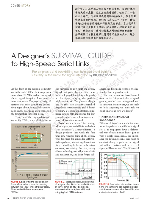
ferential impedance from the spacing between two .005” wide stripline traces. Simulated with Polar InstrumentsSI8000.of a signal after 26 inches and 40 inchesof travel down an FR-4 backplane,measured with an Agilent VNA andusing Agilent PLTS software.FIGURE 3.Conductor attenuation from a5 mil wide stripline conductor (orange)and dielectric attenuation from FR4 witha dissipation factor of 0.02.impedance of all the traces in the board must be at the target value, typically 100 Ω, in order to assure acceptable received signal amplitude and rise time.This is primarily achieved by the selection of line widths, spacing, dielec-tric thickness and knowing the dielectric constant of the laminate materials. The only way of accurately balancing the board stackup and evaluating the toler-ance buildup is with a 2D field solver .FIGURE 1explores how the spacing between two stripline traces affects their differential impedance. An easy-to-use,accurate 2D field solver is an essential tool to survive in this new regime.It is not the losses in the intercon-nects that cause problems in high-speed serial links – it is the frequency depend-ency of the losses. Both conductor loss and dielectric loss absorb more of the higher-frequency components than of the low-frequency components. This means that if you launch an ideal square wave into an interconnect, the rise time will degrade and get longer as it propa-gates, because the higher frequencies that make up the sharp edge are removed. This is illustrated in FIGURE 2.This rise time degradation causes most of the significant problems with high-speed serial interconnects, such as intersymbol interference (ISI), deter-ministic jitter and collapse of the eye diagram. It can be most easily described as the attenuation or loss in the signal as a function of frequency.Conductor loss is frequency-dependent due to skin depth effects.The cross-sectional area for current to travel through a conductor decreases into a thinner and thinner perimeter shell as frequency goes up. This increases the series resistance of boththe signal and return conductors at higher frequency.The only way to reduce the losses from the conductors’ series resistance is by using wider lines. But to use wider lines while still maintaining the target impedance also requires either thicker dielectric layers or lower dielectric constant.Of course, there is a limit to the total thickness of a board. With as many as 40 layers, in .250˝total thickness, the maximum dielectric thickness is on the order of .006˝already. And thicker boards will be more expensive due to material and drilling costs. Further , as we shall see, a thicker board also means longer via stubs, which will cause addi-tional signal integrity problems.Balancing the widest line for lowest rise time degradation, thinnest total board and acceptable cost can only be done with a simulation tool that includes lossy line effects, such as Men-tor Graphics HyperLynx or Agilent Technologies ADS.The second source of frequency-dependent loss comes from the dissipa-tion factor of the laminate. This mate-rial property is a measure of the dipoles in the laminate, which can rotate in the applied field of the signal and suck out energy from the signal.The higher signal frequency compo-nents will rotate the dipoles faster and cause more heat generation. Even though the dissipation factor of most materials is constant with frequency,the attenuation from the dissipation factor will increase with higher fre-quency. A low dissipation factor will minimize the rise time degradation.Insertion loss is a common metric to quantify the frequency-dependentloss of a signal as it propagates down an interconnect. This can be further refined as the attenuation in dB per inch of interconnect. A larger and more negative dissipation factor will mean less high-frequency signal and longer rise time, a bad thing. FIGURE 3shows an example of the insertion loss for both conductor loss and dielectric loss.As a rough rule of thumb, with many popular SERDES chips the typical acceptable attenuation might be as high as -10 dB at the bandwidth of the high-speed serial link, which is about half the bit rate. For a XAUI interface, at 3.125Gbps the bandwidth is about 1.6 GHz.If the interconnect length were 40 inch-es, the acceptable attenuation per length would be about -10 dB/40 inches, or ~ -0.25 dB/inch, at 1.6 GHz.In the example above, the total attenuation from the conductor loss and dielectric loss would be -0.12 dB/inch +-0.15 dB/inch = -0.27 dB/inch. This is above the estimated acceptable limit,which suggests a marginal design.For a robust design, either the line width must be increased, the dissipa-tion factor decreased, the interconnect length decreased, the SERDES noise margin increased, or silicon processing (i.e., pre-emphasis in the drivers)would have to be used.The Power of Pre-emphasisThe problem with attenuation in inter-connects isn’t the attenuation – it’s the frequency dependence that causes rise time degradation. If we know how much the higher frequencies will be attenuated and put an extra amount of these into the signal when it is launched, we might be able to see asharper rise time at the receiver. TheFIGURE unched signal with pre-emphasis from an Altera Stratix GX FPGA. (Figures 4, 5 and 6 courtesy ofAltera Corp.)FIGURE 5. Eye diagram of a XAUI sig-nal received after 57 inches in an FR-4backplane trace.The signal is unusable.FIGURE 6. The same FR-4 interconnect,57 inches in length, as in Figure 3, but with pre-emphasis used in the driver,utilizing the Altera Stratix GX FPGA.technique of adding high-frequency components into the launched signal is called pre-emphasis.An example of the time domain waveform of the launched signal with pre-emphasis is shown in FIGURE 4.There is an extra pulse at the tran-sitions. When this signal travels down the interconnect, the extra high-fre-quency components will be absorbed, flattening the waveform back into a more normal looking waveform. Pre-emphasis is a powerful technique of recovering a signal at the far end of a lossy line.In FIGURE 5is displayed the eye diagram of a XAUI signal, received after 57 inches in an FR-4 intercon-nect. There is so much frequency-dependent attenuation that all the bits are grossly distorted and cannot be read with any certainty. This intercon-nect is completely unusable.However, with pre-emphasis, extra high-frequency components are added to the signal and the frequency-dependent attenuation sucks out these extra components, leaving behind a much more usable signal. This is shown in FIGURE 6.The combination of conventional FR-4 boards and pre-emphasis in the drivers is a powerful combination for designing successful high-speed serial links. The higher the bandwidth, the greater the need for wider lines, lower dissipation factor and silicon processing.Though pre-emphasis can over-come losses in the interconnect, it can-not overcome the sharp resonances from via stubs. Ultimately, these stubs will be a fundamental limit to the bit rate for backplane interconnects.If conductor and dielectric loss were the only processes decreasing the insertion loss with frequency, pre-emphasis could compensate. Unfortu-nately, the stubs created by through vias can act as resonators and absorb a very large amount of the signal energy in narrow frequency bands. An exam-ple of the measured insertion loss of a backplane channel with and without a via stub is shown in FIGURE 7.The resonator is created when a signal uses a through via to transition from two closely spaced layers, such as between layers 1 and 4 or 2 and 5 in aBackdrilled via200-mil through-hole via stub0-20-40-60-80-10005101520Even lower frequency bit rates can suffer from via stub resonances, if their bandwidths are riding on the edge of the resonance curve. The most effective way of eliminating this problem is to move the via stub resonant frequency as high as possible, by using as short a via stub as possible. This can be done by removing NFPs from unused layers, limiting layer transitions to those near the outer layers, and backdrilling any stubs that might be left.Backdrilling is the process of re-drilling the bottom of the via with an oversized drill bit, after the through via has been plated. This removed the plat-ed through hole that is not being used and eliminates the resonating stub. FIG-URE 8shows an example of an as-fab-ricated through-hole via in an 18-layer board, and a similar via that has been backdrilled to remove the long stub.Backdrilling has become the de facto standard in all high-performance backplanes used in systems at 5 Gbps and above. To allow scalability of a backplane that may be first used at 2.5 Gbps or even 3.125 Gbps, so that it could be used later in life at 5 Gbps, backdrilling is often employed. This way, higher bit rate cards can be plugged into this legacy backplane and still operate acceptably.Beginning of an EraIn this new era of high-speed serial links operating at 2 Gbps and above, a new set of signal integrity concerns must be considered for a system to work the first time. In addition to all the other signal integrity problems like terminations and topologies, crosstalk, ground bounce and power distribu-tion, now we must design out differen-tial impedance problems, deal with losses and include via stub effects.To survive this new set of mine-fields requires new skills, new tools and new technologies. The elements of survival include the use of 2D field solvers to accurately design the stackup and routing for differential pairs, the selection of optimal dielectric materials with low dielectric constant to allow wide lines and thin boards, low dissi-pation factor for low insertion loss and the use of silicon processing such as pre-emphasis. Finally, techniques to minimize the length of via stubs suchas backdrilling are essential.Now interconnects are not onlynot transparent but are the dominantfactor determining whether a large,high-performance system will work thefirst time, every time. By paying carefulattention to all of these importantissues, you can be successful in this eraand earn the right to face the chal-lenges of the next generation of high-performance systems. PCD&MERIC BOGATIN is the CTO at IDI, andpresident of Bogatin Enterprises. He canbe reached at eric@.REFERENCES1.This paper is based on Online Lecture 184,A Designer’s Survival Guide to High-SpeedSerial Links, posted on www.bethe. To view this lecture for free,enter coupon code PCDM0507.2.Bogatin, Eric, Signal Integrity - Simplified,Prentice Hall, 2003.。
常微分方程中的英文单词和短语

常微分方程
Ordinary Differential Equtions
第一章 基本概念
Chapter 1 Basic Concepts
常微分方 程
阶 线性 非线性 偏微分方 程
通解 特解 初值条件 初值问题 柯西问题 几何解释 积分曲线 线素 线素场 方向场 等斜线 对称形式 奇异点 通积分
boundary finite closed interval open set finite semi-open interval
Lagrange formula
l ocal finite covering theorem
bar area monotone decreasing sectorial area comparability solution minimum solution maximum solution sl ope
topological dynamical system
differential dynamical system
stability of solution Liapunov stability
asymptotic stability asymptotic stability field attraction domain globe asymptotic stability
第六章 线 性 微 分 方 程 组
Chapter 6 Linear Differential Equations
存在和唯一 性定理 齐次线性微 分方程组 基本解组 朗斯基行列 式 刘维尔公 式 解矩阵 基解矩阵 常数矩阵 非齐次线性 微分方程 组 常数列向 量 常数变异公 式 计算公式 结构公式 常系数线性 微分方程 组 矩阵指数函 数 标准基解矩 阵 若尔当标准 型 矩阵函数 实值解 复值解 代数余子 式 特征方程 算子式 算子多项 式 拉普拉斯逆 变换
Phase-field 方法的基本思路-特点

Phase-field 方法的基本思路\特点摘要:本篇文章的主要内容是关于phase-field方法的,介绍了相场法的基本思想,简述了相场法的计算方法及优缺点,还对相场法的应用情况作了概述。
关键字:相场法两相计算方法应用Abstract: The main content of this article is about the phase-field method, which introduces the basic idea of phase field method, the calculation method and the advantages and disadvantages of the phase field method, and an overview of the application of the phase field method.Key words: phase field method; two-phase flow; calculation method; application 1相场法的基本思想相场方法是以金兹堡—朗道理论为基础,用微分方程来体现扩散、有序化势和热力学驱动的综合作用。
相场是一种计算技术,它能使研究者直接模拟微观组织的形成。
因此,相场法也称为直接的微观组织模拟。
与其他方法不同,相场法引入了相场变量这个概念来描述系统在空间/时间上每个位置的物理状态。
相场变量用φ(r,t)表示,其中r代表空间,t代表时间,在液相区,φ(r,t)=-1;在固相区φ(r,t)=1;而在固液两相区,φ(r,t)的值在-1~1之间变化。
2相场模拟中的计算方法2.1有限差分法有限差分法的发展已比较的成熟,并且十分重要的是它的程序结构十分简单。
人们相继实现了对枝晶生长定性和定量模拟,并且与预测结果十分吻合。
在国内,分别实现了对镍的等轴枝晶生长、铝的枝晶生长和对铝铜合金的生长过程的模拟。
线性系统课后答案第2章
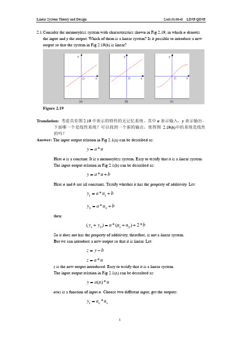
2.1 Consider the memoryless system with characteristics shown in Fig 2.19, in which u denotes the input and y the output. Which of them is a linear system? Is it possible to introduce a new output so that the system in Fig 2.19(b) is linear?Figure 2.19Translation: 考虑具有图2.19中表示的特性的无记忆系统。
其中u 表示输入,y 表示输出。
下面哪一个是线性系统?可以找到一个新的输出,使得图2.19(b)中的系统是线性的吗?Answer: The input-output relation in Fig 2.1(a) can be described as:u a y *=Here a is a constant. It is a memoryless system. Easy to testify that it is a linear system. The input-output relation in Fig 2.1(b) can be described as:b u a y +=*Here a and b are all constants. Testify whether it has the property of additivity. Let: b u a y +=11*b u a y +=22*then:b u u a y y *2)(*)(2121++=+So it does not has the property of additivity, therefore, is not a linear system.But we can introduce a new output so that it is linear. Let:b y z -=u a z *=z is the new output introduced. Easy to testify that it is a linear system.The input-output relation in Fig 2.1(c) can be described as:u u a y *)(=a(u) is a function of input u . Choose two different input, get the outputs:111*u a y =222*u a y =Assure:21a a ≠then:221121**)(u a u a y y +=+So it does not has the property of additivity, therefore, is not a linear system.2.2 The impulse response of an ideal lowpass filter is given by)(2)(2sin 2)(00t t t t t g --=ωωω for all t , where w and to are constants. Is the ideal lowpass filter causal? Is is possible to built the filter in the real world?Translation: 理想低通滤波器的冲激响应如式所示。
最优控制理论第七章

State Equation: Sale expressed in terms of advertising (which is a control variable) Objective: Profit maximization
Defining as the elasticity of demand with respect to goodwill and using (7.3), (7.5), and (7.9), we can derive ( sto obtain the optimal long-run stationary equilibrium or turnpike . That is, we obtain from (7.8) by using . We then set and in (7.9). Finally, from (7.11) and (7.9), or also the singular level can be obtained as
Because of these conditions it is clear that for a given G0 , a choice of 0 such that (0 ,G0 ) is in Regions II and III, will not lead to a path converging to the turnpike point . On the other hand, the choice of (0 ,G0 ) in Region I when or (0 ,G0 ) in Region IV when , can give a path that converges to From a result in Coddington and Levinson(1955), it can be shown that at least in the neighborhood of , there exists a locus of optimum starting points . Given , we choose 0 on the saddle point path in Region I of figure 7.3. Clearly, the initial control u*(0)=f1(0). Furthermore, (t) is increasing and by (7.17), u(t) is increasing, so that in this case the optimal policy is to advertise at a low rate initially and
黄铁矿和磁黄铁矿成因区别
ABSTRACT. The origin in rocks of the common iron sulphides, pyrrhotine, Fe 1 xS and pyrite, FeS2 and their behaviour during geochemical processes is best considered using the simplified redox reaction: 2FeS ~-~FeS2 + Fe 2+ + 2e . Thus pyrrhotine is more reduced than pyrite and is the stable iron sulphide formed from magmas except where relatively high oxygen fugacities result from falling pressure or hydrothermal alteration. Pyrite, on the other hand, is the stable iron sulphide in even the most reduced sedimentary rocks where it usually forms during diagenesis through bacteriogenic reduction of sulphate; it is stable throughout the pressure/temperature range endured by normal sedimentary rocks. Pyrrhotine after pyrite or sulphate in metasediments of regional metamorphic origin results mainly from progressive reduction on metamorphism due to the presence of graphite-buffered fluids. Pyrrhotine and/or pyrite may be precipitated from hydrothermal solutions on epigenetic or syngenetic mineralization but pyrrhotine will only be preserved if protected from oxidation to pyrite or to more oxidized species. Exhalative pyrrhotine appears to have been more common in Precambrian times and/or in depositional environments destined to become regionally metamorphosed. FeS can be considered to be the soluble iron sulphide, rather than FeS2, in reduced aqueous systems although pyrite may precipitate from solution as a result of redox reactions. The relatively soluble nature of FeS explains the observed mobility of iron sulphides in all rock types.
Disconnecting EHV shunt reactors by SF and air-blast breakers
Disconnecting EHV shunt reactors by SF 6 and air-blast breakersLászló PriklerDepartment of Electric Power Systems Technical University of Budapes, HungaryEgry J. u. 18. H-1111 Budapest Phone/Fax: +36 1 463 3015/-3013 E-mail: priki@vmt.bme.hu1 IntroductionAt EHV level shunt reactors are applied to regulate the reactive power balance of a system by means of compensating for the surplus reactive power generation of transmission lines.Reactors are normally disconnected at heavy load and are connected to the lines at periods of low load. Consequently, frequent switching is a significant characteristics of reactors. The main insulation of reactors can be overstressed if the breaker has high current chopping character. Furthermore, if a conventional arrester operates as a consequence of current chopping, or a restrike occurs during the switching-off operation, the turn-to-turn insulation of the reactor can also be jeopardized by the steep voltage change. In this case study a comprehensive and a simplified EMTP model of the reactor are introduced. The computer model has been validated in field experiments.2 Case descriptionOne line diagram of the 750/400 kV Albertirsa substation in Hungary is shown on Fig. 1. Two sets of 330 Mvar reactors are connected to the transmission line terminal via long bus-bars.After 10 years of operation the air-blast breakers have been replaced by SF 6 insulated devices. The new breakers are equipped with a point-on-wave control device in order to eliminate breaker restrikes otherwise could be arosen. The case studies shown here were part of a two-years research aimed at comparing the breaker characteristics and the specification of the control device.∆∆C.B.165m bus-bar750 kV400 kV750 kVline1100 MVA1100 MVA330 MVA330 MVAtested installationFig. 1 - One line diagram of the 750/400 kV substation3 AssumptionsModel of the supply side network: The 750 kV transmission line and the transformer were taken into account individually in the model, while the remaining part of the 400 kV grid has been represented by an inductance. An inductively coupled linear, unsaturated BCTRAN model represents the 1100 MVA auto-transformer in the model. The capacitances of the transformer and of the substation bus-bars are also significant, so the network model has been completed by these elements.Circuit breaker models: Time controlled switch with pre-defined current chopping level, as the most simple alternative to breaker modelling, has been applied. It also applies to the old,air-blast type breaker and the new SF 6 insulated unit, too. In the case of the air-blast type, 70Amps were applied, based on previous field measurements. The modern SF 6 breakers have been characterised by a much smaller value (I ch =3 10 Amps), calculated from the "chopping number" of the breaker, which can be obtained from the manufacturer. Reignitions betweeen the moving contacts were simulated by a voltage controlled switch in parallel with the main switch.Lightning arrester model: Both the Type-92 and Type-99 non-linear resistor model of EMTP can be used for simulation of conventional (gaped) and metal oxide arresters. There were no difference in calculated values using different arrester models, however the simulation speed is slower by a factor of two, using model 92. Accurate modelling of arrester non-linearity in small (<100A) current region has been found to be essential.Reactor bus-bar: Three phase, non-transposed, frequency dependent line model (Jmarti line) gave the more precise representation. Application of this model, however requires very small simulation time step, so this model is preferable to use only in case of restrike studies,when the role of travelling waves along the bus-bar is fundamental. Otherwise three phase nominal PI circuit, with parameters calculated at the free oscillation frequency of the reactor voltage (870 Hz) has been used.Simplified shunt reactor model: A simple reactor model is a two port equivalent of an inductance in parallel with a capacitor. The value of the capacitor can be predicted by substituting the frequency of the free oscillation f and the value of the reactor inductance L into the following formula:()C f L=−4221πWhere L is the linear, unsaturated value of the reactor inductance, because the iron core has air gaps, resulting in high saturation level. The bushing capacitance (C b ) and the bus-bar capacitances (C bb ) also take part in the oscillation, so the capacitance of the reactor (C L ) can be defined as:C C C C L b bb=−−The copper losses of the winding, the iron and dielectric losses of the core can be represented by lumped serial/parallel resistances as shown in Fig. 2RLr C LC bC bbFig 2.- Simple model of the reactor-busbar circuitDetailed model of the reactor : The simplified reactor model provides output voltages at the high voltage terminal only and no information is available about the magnitude of internal stresses. In order to be able to predict the local overvoltages a more sophisticated reactor model has to be used. This comprehensive reactor model (Fig.3) is based on ´n´ part inductively coupled (51, 52...) element of EMTP. The homogeneous single-layer winding consists of n pieces of part-windings. Each of them has self inductance (L ii ) and n-1 mutual inductances (M ij ) to the others as it is shown in Fig. 4. The inductance matrix L of the reactor contains n pieces of L ii in the main diagonal and n-i pieces of L ii multiplied by the i-th power of the coupling factor in the i-th parallel sub-diagonal. Accordingly, the elements of L can be derived from the known reactor inductance.L 11r 11R 11K 0,1C 11R K C L 22L nnr 22R 22K 1,2nnr n-1,n nnn-1,n-1C nnC 22M 12M 1nH.V.terminaln-112Fig 3.- Detailed model of the reactor4 Used ATP components3 phase , BCTRAN linear transformer, Lumped RLC, Time-controlled switch, 3 phase distributed transposed line, Type 51..52 RL coupled element, Type 92 and 99 non-linear resistor5 Data and EMTP model6H10nF60nF22nF750 kV tr. linereactor bus-bar150Ω42030.3uF∆400 kV supply network Ssc=8000MVAFig. 4 - Single phase diagram of the EMTP model6 Critical parameters- Frequency at which the parameters of the 3 phase PI is calculated. (base frequency of the reactor oscillation (870 Hz) in that case- IMARGIN of the switches, representing the current chopping level of breakers (SF6breaker: 8-10 Amps, Air blast breaker: 60-80 A)- Accurate modelling of arrester non-linearity in small (<100A) current region7 Simulation results and verificationThe EMTP model described above can be used in case studies where the dominant frequency component is less then 100 kHz. Such kind of studies are:- calculation of TRV stresses at reactors and at the breaker- comparision of the main characteristics of different type of breakers- specification of the breaker parameters (mechanical as well as electrical)- development of controlled switching strategy- calculation of voltage distribution along the reactor windingThe model has been verified using field measurements. Several switching operations were recorded using a digital disturbance recorder before pushing into operation the new SF 6circuit breakers and following the breaker replacement. Two typical oscillograms recorded at the field tests are shown in Fig.5 and Fig.6. Disconnecting reactors by an air blast type breaker resulted in high overvoltages and arresters operated in each phase and at everyswitching off cycle. Reignitions also occurred frequently. The new SF 6 breaker produces much lower overvoltages and no arrester operation were being observed. However reignitions without controlling the switching operation can not be eliminated completely.The computer simulation produces very similar reactor voltage oscillations than that of the field test records (see Fig. 7 and 8).Verification status of the caseField test TNAOther program AnalyticalFig 5 - Measured phase to ground reactorvoltages disconnecting reactors by SF 6breaker010203040-600-400-200 0 200 400 600U [kV]T [ms]010203040-600-400-200 0 200 400 600U [kV]T [ms]10203040-600-400-200 0 200 400 600U [kV]T [ms]Fig 7 - Calculated phase to ground reactor voltages disconnecting reactors by SF 6breakerphase Aphase Bphase CFig 6 - Measured phase to ground voltages disconnecting reactors by air-blast breaker0102030 01000U [kV]T [ms]Fig 8 - Calculated phase to ground voltages disconnecting reactors by air blast breaker8 References[1] Andersen at al.: Synchronous energizing of shunt reactors and shunt capacitors, CIGREpaper 13-12, 1988[2] IEC Technical Report No.1233, High voltage alternating current circuit breakers, inductiveload switching, 1993[3] L.Prikler, G.Ban, Gy.Banfai: EMTP models for simulation of shunt reactor switchingtransients, Electrical Power & Energy Systems , Vol. 19, No. 4, May 1997. pp. 235-240AppendixName of ATP input file:SW_REACT.ATPName of ATPDRAW file:not availableAvailability: HTTP://www.vmt.bme.hu/eeug/casebook/case_32.htmBEGIN NEW DATA CASEC ATP CASE STUDIES: SHUNT REACTOR SWITCHINGC REF: ATP Case-study workbook: X.4.10.5E-6 35.0E-31 20 -1 15 5 20 20 100 100C ---- EQUIVALENT SUPPLY NETWORK REDUCED TO THE 750 KV BUS -----AGENA AIS7A 150.AGENA AIS7A 530.AGENB AIS7B 150.AGENB AIS7B 530.AGENC AIS7C 150.AGENC AIS7C 530.C --------------- SHUNT REACTORS -------------------------------AISFA 20. 6000. 1 AISFB 20. 6000. 1 AISFC 20. 6000. 1 AISFA 2.0E+6AISFB 2.0E+6AISFC 2.0E+6AISFA .0037AISFB .0037AISFC .0037C ----- RVMK TYP. 750 kV CONVENTIONAL ARRESTER -----------------99 AISFA 1250. 7 10.001 150.00.005 210.00.010 250.00.020 300.00.040 360.00.100 400.01.000 1020.09999. SINGLE FLASH99 AISFB AISFA 1250. 7 199 AISFC AISFA 1250. 7 1C --------- REACTOR BUS-BAR, PI MODEL AT 870 HZ -----------------$UNITS, 870. , 870. ,$VINTAGE, 11 AISMA AISFA 7.80619215E-02 1.02699335E+00 8.91459084E+002 AISMB AISFB 6.60560152E-02 3.46436665E-01 -2.13971630E+007.80645558E-02 1.02695225E+00 9.35844488E+003 AISMC AISFC 6.36697132E-02 2.35679712E-01 -7.90769926E-016.60560152E-02 3.46436665E-01 -2.13971630E+007.80619215E-02 1.02699335E+00 8.91459084E+00$VINTAGE, 0$UNITS, 0.0 , 0.0 ,BLANKC ---------------- CIRCUIT BREAKERS -----------------------------AIS7A AISMA -1.E-3 3.0E-3 0.080AIS7B AISMB -1.E-3 1.0E-3 0.060AIS7C AISMC -1.E-3 0.0E-3 0.080BLANKC ------------------ GENERATORS --------------------------------14 AGENA 613. 50. -150. -0.0114 AGENB 613. 50. 90. -0.0114 AGENC 613. 50. -30. -0.01BLANKAISFA AISFB AISFCBLANKBEGIN NEW DATA CASEBLANKBLANK。
离散数学中英文名词对照表
离散数学中英⽂名词对照表离散数学中英⽂名词对照表外⽂中⽂AAbel category Abel 范畴Abel group (commutative group) Abel 群(交换群)Abel semigroup Abel 半群accessibility relation 可达关系action 作⽤addition principle 加法原理adequate set of connectives 联结词的功能完备(全)集adjacent 相邻(邻接)adjacent matrix 邻接矩阵adjugate 伴随adjunction 接合affine plane 仿射平⾯algebraic closed field 代数闭域algebraic element 代数元素algebraic extension 代数扩域(代数扩张)almost equivalent ⼏乎相等的alternating group 三次交代群annihilator 零化⼦antecedent 前件anti symmetry 反对称性anti-isomorphism 反同构arboricity 荫度arc set 弧集arity 元数arrangement problem 布置问题associate 相伴元associative algebra 结合代数associator 结合⼦asymmetric 不对称的(⾮对称的)atom 原⼦atomic formula 原⼦公式augmenting digeon hole principle 加强的鸽⼦笼原理augmenting path 可增路automorphism ⾃同构automorphism group of graph 图的⾃同构群auxiliary symbol 辅助符号axiom of choice 选择公理axiom of equality 相等公理axiom of extensionality 外延公式axiom of infinity ⽆穷公理axiom of pairs 配对公理axiom of regularity 正则公理axiom of replacement for the formula Ф关于公式Ф的替换公式axiom of the empty set 空集存在公理axiom of union 并集公理Bbalanced imcomplete block design 平衡不完全区组设计barber paradox 理发师悖论base 基Bell number Bell 数Bernoulli number Bernoulli 数Berry paradox Berry 悖论bijective 双射bi-mdule 双模binary relation ⼆元关系binary symmetric channel ⼆进制对称信道binomial coefficient ⼆项式系数binomial theorem ⼆项式定理binomial transform ⼆项式变换bipartite graph ⼆分图block 块block 块图(区组)block code 分组码block design 区组设计Bondy theorem Bondy 定理Boole algebra Boole 代数Boole function Boole 函数Boole homomorophism Boole 同态Boole lattice Boole 格bound occurrence 约束出现bound variable 约束变量bounded lattice 有界格bridge 桥Bruijn theorem Bruijn 定理Burali-Forti paradox Burali-Forti 悖论Burnside lemma Burnside 引理Ccage 笼canonical epimorphism 标准满态射Cantor conjecture Cantor 猜想Cantor diagonal method Cantor 对⾓线法Cantor paradox Cantor 悖论cardinal number 基数Cartesion product of graph 图的笛卡⼉积Catalan number Catalan 数category 范畴Cayley graph Cayley 图Cayley theorem Cayley 定理center 中⼼characteristic function 特征函数characteristic of ring 环的特征characteristic polynomial 特征多项式check digits 校验位Chinese postman problem 中国邮递员问题chromatic number ⾊数chromatic polynomial ⾊多项式circuit 回路circulant graph 循环图circumference 周长class 类classical completeness 古典完全的classical consistent 古典相容的clique 团clique number 团数closed term 闭项closure 闭包closure of graph 图的闭包code 码code element 码元code length 码长code rate 码率code word 码字coefficient 系数coimage 上象co-kernal 上核coloring 着⾊coloring problem 着⾊问题combination number 组合数combination with repetation 可重组合common factor 公因⼦commutative diagram 交换图commutative ring 交换环commutative seimgroup 交换半群complement 补图(⼦图的余) complement element 补元complemented lattice 有补格complete bipartite graph 完全⼆分图complete graph 完全图complete k-partite graph 完全k-分图complete lattice 完全格composite 复合composite operation 复合运算composition (molecular proposition) 复合(分⼦)命题composition of graph (lexicographic product)图的合成(字典积)concatenation (juxtaposition) 邻接运算concatenation graph 连通图congruence relation 同余关系conjunctive normal form 正则合取范式connected component 连通分⽀connective 连接的connectivity 连通度consequence 推论(后承)consistent (non-contradiction) 相容性(⽆⽭盾性)continuum 连续统contraction of graph 图的收缩contradiction ⽭盾式(永假式)contravariant functor 反变函⼦coproduct 上积corank 余秩correct error 纠正错误corresponding universal map 对应的通⽤映射countably infinite set 可列⽆限集(可列集)covariant functor (共变)函⼦covering 覆盖covering number 覆盖数Coxeter graph Coxeter 图crossing number of graph 图的叉数cuset 陪集cotree 余树cut edge 割边cut vertex 割点cycle 圈cycle basis 圈基cycle matrix 圈矩阵cycle rank 圈秩cycle space 圈空间cycle vector 圈向量cyclic group 循环群cyclic index 循环(轮转)指标cyclic monoid 循环单元半群cyclic permutation 圆圈排列cyclic semigroup 循环半群DDe Morgan law De Morgan 律decision procedure 判决过程decoding table 译码表deduction theorem 演绎定理degree 次数,次(度)degree sequence 次(度)序列derivation algebra 微分代数Descartes product Descartes 积designated truth value 特指真值detect errer 检验错误deterministic 确定的diagonal functor 对⾓线函⼦diameter 直径digraph 有向图dilemma ⼆难推理direct consequence 直接推论(直接后承)direct limit 正向极限direct sum 直和directed by inclution 被包含关系定向discrete Fourier transform 离散 Fourier 变换disjunctive normal form 正则析取范式disjunctive syllogism 选⾔三段论distance 距离distance transitive graph 距离传递图distinguished element 特异元distributive lattice 分配格divisibility 整除division subring ⼦除环divison ring 除环divisor (factor) 因⼦domain 定义域Driac condition Dirac 条件dual category 对偶范畴dual form 对偶式dual graph 对偶图dual principle 对偶原则(对偶原理) dual statement 对偶命题dummy variable 哑变量(哑变元)Eeccentricity 离⼼率edge chromatic number 边⾊数edge coloring 边着⾊edge connectivity 边连通度edge covering 边覆盖edge covering number 边覆盖数edge cut 边割集edge set 边集edge-independence number 边独⽴数eigenvalue of graph 图的特征值elementary divisor ideal 初等因⼦理想elementary product 初等积elementary sum 初等和empty graph 空图empty relation 空关系empty set 空集endomorphism ⾃同态endpoint 端点enumeration function 计数函数epimorphism 满态射equipotent 等势equivalent category 等价范畴equivalent class 等价类equivalent matrix 等价矩阵equivalent object 等价对象equivalent relation 等价关系error function 错误函数error pattern 错误模式Euclid algorithm 欧⼏⾥德算法Euclid domain 欧⽒整环Euler characteristic Euler 特征Euler function Euler 函数Euler graph Euler 图Euler number Euler 数Euler polyhedron formula Euler 多⾯体公式Euler tour Euler 闭迹Euler trail Euler 迹existential generalization 存在推⼴规则existential quantifier 存在量词existential specification 存在特指规则extended Fibonacci number ⼴义 Fibonacci 数extended Lucas number ⼴义Lucas 数extension 扩充(扩张)extension field 扩域extension graph 扩图exterior algebra 外代数Fface ⾯factor 因⼦factorable 可因⼦化的factorization 因⼦分解faithful (full) functor 忠实(完满)函⼦Ferrers graph Ferrers 图Fibonacci number Fibonacci 数field 域filter 滤⼦finite extension 有限扩域finite field (Galois field ) 有限域(Galois 域)finite dimensional associative division algebra有限维结合可除代数finite set 有限(穷)集finitely generated module 有限⽣成模first order theory with equality 带符号的⼀阶系统five-color theorem 五⾊定理five-time-repetition 五倍重复码fixed point 不动点forest 森林forgetful functor 忘却函⼦four-color theorem(conjecture) 四⾊定理(猜想)F-reduced product F-归纳积free element ⾃由元free monoid ⾃由单元半群free occurrence ⾃由出现free R-module ⾃由R-模free variable ⾃由变元free-?-algebra ⾃由?代数function scheme 映射格式GGalileo paradox Galileo 悖论Gauss coefficient Gauss 系数GBN (G?del-Bernays-von Neumann system)GBN系统generalized petersen graph ⼴义 petersen 图generating function ⽣成函数generating procedure ⽣成过程generator ⽣成⼦(⽣成元)generator matrix ⽣成矩阵genus 亏格girth (腰)围长G?del completeness theorem G?del 完全性定理golden section number 黄⾦分割数(黄⾦分割率)graceful graph 优美图graceful tree conjecture 优美树猜想graph 图graph of first class for edge coloring 第⼀类边⾊图graph of second class for edge coloring 第⼆类边⾊图graph rank 图秩graph sequence 图序列greatest common factor 最⼤公因⼦greatest element 最⼤元(素)Grelling paradox Grelling 悖论Gr?tzsch graph Gr?tzsch 图group 群group code 群码group of graph 图的群HHajós conjecture Hajós 猜想Hamilton cycle Hamilton 圈Hamilton graph Hamilton 图Hamilton path Hamilton 路Harary graph Harary 图Hasse graph Hasse 图Heawood graph Heawood 图Herschel graph Herschel 图hom functor hom 函⼦homemorphism 图的同胚homomorphism 同态(同态映射)homomorphism of graph 图的同态hyperoctahedron 超⼋⾯体图hypothelical syllogism 假⾔三段论hypothese (premise) 假设(前提)Iideal 理想identity 单位元identity natural transformation 恒等⾃然变换imbedding 嵌⼊immediate predcessor 直接先⾏immediate successor 直接后继incident 关联incident axiom 关联公理incident matrix 关联矩阵inclusion and exclusion principle 包含与排斥原理inclusion relation 包含关系indegree ⼊次(⼊度)independent 独⽴的independent number 独⽴数independent set 独⽴集independent transcendental element 独⽴超越元素index 指数individual variable 个体变元induced subgraph 导出⼦图infinite extension ⽆限扩域infinite group ⽆限群infinite set ⽆限(穷)集initial endpoint 始端initial object 初始对象injection 单射injection functor 单射函⼦injective (one to one mapping) 单射(内射)inner face 内⾯inner neighbour set 内(⼊)邻集integral domain 整环integral subdomain ⼦整环internal direct sum 内直和intersection 交集intersection of graph 图的交intersection operation 交运算interval 区间invariant factor 不变因⼦invariant factor ideal 不变因⼦理想inverse limit 逆向极限inverse morphism 逆态射inverse natural transformation 逆⾃然变换inverse operation 逆运算inverse relation 逆关系inversion 反演isomorphic category 同构范畴isomorphism 同构态射isomorphism of graph 图的同构join of graph 图的联JJordan algebra Jordan 代数Jordan product (anti-commutator) Jordan乘积(反交换⼦)Jordan sieve formula Jordan 筛法公式j-skew j-斜元juxtaposition 邻接乘法Kk-chromatic graph k-⾊图k-connected graph k-连通图k-critical graph k-⾊临界图k-edge chromatic graph k-边⾊图k-edge-connected graph k-边连通图k-edge-critical graph k-边临界图kernel 核Kirkman schoolgirl problem Kirkman ⼥⽣问题Kuratowski theorem Kuratowski 定理Llabeled graph 有标号图Lah number Lah 数Latin rectangle Latin 矩形Latin square Latin ⽅lattice 格lattice homomorphism 格同态law 规律leader cuset 陪集头least element 最⼩元least upper bound 上确界(最⼩上界)left (right) identity 左(右)单位元left (right) invertible element 左(右)可逆元left (right) module 左(右)模left (right) zero 左(右)零元left (right) zero divisor 左(右)零因⼦left adjoint functor 左伴随函⼦left cancellable 左可消的left coset 左陪集length 长度Lie algebra Lie 代数line- group 图的线群logically equivanlent 逻辑等价logically implies 逻辑蕴涵logically valid 逻辑有效的(普效的)loop 环Lucas number Lucas 数Mmagic 幻⽅many valued proposition logic 多值命题逻辑matching 匹配mathematical structure 数学结构matrix representation 矩阵表⽰maximal element 极⼤元maximal ideal 极⼤理想maximal outerplanar graph 极⼤外平⾯图maximal planar graph 极⼤平⾯图maximum matching 最⼤匹配maxterm 极⼤项(基本析取式)maxterm normal form(conjunctive normal form) 极⼤项范式(合取范式)McGee graph McGee 图meet 交Menger theorem Menger 定理Meredith graph Meredith 图message word 信息字mini term 极⼩项minimal κ-connected graph 极⼩κ-连通图minimal polynomial 极⼩多项式Minimanoff paradox Minimanoff 悖论minimum distance 最⼩距离Minkowski sum Minkowski 和minterm (fundamental conjunctive form) 极⼩项(基本合取式)minterm normal form(disjunctive normal form)极⼩项范式(析取范式)M?bius function M?bius 函数M?bius ladder M?bius 梯M?bius transform (inversion) M?bius 变换(反演)modal logic 模态逻辑model 模型module homomorphism 模同态(R-同态)modus ponens 分离规则modus tollens 否定后件式module isomorphism 模同构monic morphism 单同态monoid 单元半群monomorphism 单态射morphism (arrow) 态射(箭)M?bius function M?bius 函数M?bius ladder M?bius 梯M?bius transform (inversion) M?bius 变换(反演)multigraph 多重图multinomial coefficient 多项式系数multinomial expansion theorem 多项式展开定理multiple-error-correcting code 纠多错码multiplication principle 乘法原理mutually orthogonal Latin square 相互正交拉丁⽅Nn-ary operation n-元运算n-ary product n-元积natural deduction system ⾃然推理系统natural isomorphism ⾃然同构natural transformation ⾃然变换neighbour set 邻集next state 下⼀个状态next state transition function 状态转移函数non-associative algebra ⾮结合代数non-standard logic ⾮标准逻辑Norlund formula Norlund 公式normal form 正规形normal model 标准模型normal subgroup (invariant subgroup) 正规⼦群(不变⼦群)n-relation n-元关系null object 零对象nullary operation 零元运算Oobject 对象orbit 轨道order 阶order ideal 阶理想Ore condition Ore 条件orientation 定向orthogonal Latin square 正交拉丁⽅orthogonal layout 正交表outarc 出弧outdegree 出次(出度)outer face 外⾯outer neighbour 外(出)邻集outerneighbour set 出(外)邻集outerplanar graph 外平⾯图Ppancycle graph 泛圈图parallelism 平⾏parallelism class 平⾏类parity-check code 奇偶校验码parity-check equation 奇偶校验⽅程parity-check machine 奇偶校验器parity-check matrix 奇偶校验矩阵partial function 偏函数partial ordering (partial relation) 偏序关系partial order relation 偏序关系partial order set (poset) 偏序集partition 划分,分划,分拆partition number of integer 整数的分拆数partition number of set 集合的划分数Pascal formula Pascal 公式path 路perfect code 完全码perfect t-error-correcting code 完全纠-错码perfect graph 完美图permutation 排列(置换)permutation group 置换群permutation with repetation 可重排列Petersen graph Petersen 图p-graph p-图Pierce arrow Pierce 箭pigeonhole principle 鸽⼦笼原理planar graph (可)平⾯图plane graph 平⾯图Pólya theorem Pólya 定理polynomail 多项式polynomial code 多项式码polynomial representation 多项式表⽰法polynomial ring 多项式环possible world 可能世界power functor 幂函⼦power of graph 图的幂power set 幂集predicate 谓词prenex normal form 前束范式pre-ordered set 拟序集primary cycle module 准素循环模prime field 素域prime to each other 互素primitive connective 初始联结词primitive element 本原元primitive polynomial 本原多项式principal ideal 主理想principal ideal domain 主理想整环principal of duality 对偶原理principal of redundancy 冗余性原则product 积product category 积范畴product-sum form 积和式proof (deduction) 证明(演绎)proper coloring 正常着⾊proper factor 真正因⼦proper filter 真滤⼦proper subgroup 真⼦群properly inclusive relation 真包含关系proposition 命题propositional constant 命题常量propositional formula(well-formed formula,wff)命题形式(合式公式)propositional function 命题函数propositional variable 命题变量pullback 拉回(回拖) pushout 推出Qquantification theory 量词理论quantifier 量词quasi order relation 拟序关系quaternion 四元数quotient (difference) algebra 商(差)代数quotient algebra 商代数quotient field (field of fraction) 商域(分式域)quotient group 商群quotient module 商模quotient ring (difference ring , residue ring) 商环(差环,同余类环)quotient set 商集RRamsey graph Ramsey 图Ramsey number Ramsey 数Ramsey theorem Ramsey 定理range 值域rank 秩reconstruction conjecture 重构猜想redundant digits 冗余位reflexive ⾃反的regular graph 正则图regular representation 正则表⽰relation matrix 关系矩阵replacement theorem 替换定理representation 表⽰representation functor 可表⽰函⼦restricted proposition form 受限命题形式restriction 限制retraction 收缩Richard paradox Richard 悖论right adjoint functor 右伴随函⼦right cancellable 右可消的right factor 右因⼦right zero divison 右零因⼦ring 环ring of endomorphism ⾃同态环ring with unity element 有单元的环R-linear independence R-线性⽆关root field 根域rule of inference 推理规则Russell paradox Russell 悖论Ssatisfiable 可满⾜的saturated 饱和的scope 辖域section 截⼝self-complement graph ⾃补图semantical completeness 语义完全的(弱完全的)semantical consistent 语义相容semigroup 半群separable element 可分元separable extension 可分扩域sequent ⽮列式sequential 序列的Sheffer stroke Sheffer 竖(谢弗竖)simple algebraic extension 单代数扩域simple extension 单扩域simple graph 简单图simple proposition (atomic proposition) 简单(原⼦)命题simple transcental extension 单超越扩域simplication 简化规则slope 斜率small category ⼩范畴smallest element 最⼩元(素)Socrates argument Socrates 论断(苏格拉底论断)soundness (validity) theorem 可靠性(有效性)定理spanning subgraph ⽣成⼦图spanning tree ⽣成树spectra of graph 图的谱spetral radius 谱半径splitting field 分裂域standard model 标准模型standard monomil 标准单项式Steiner triple Steiner 三元系⼤集Stirling number Stirling 数Stirling transform Stirling 变换subalgebra ⼦代数subcategory ⼦范畴subdirect product ⼦直积subdivison of graph 图的细分subfield ⼦域subformula ⼦公式subdivision of graph 图的细分subgraph ⼦图subgroup ⼦群sub-module ⼦模subrelation ⼦关系subring ⼦环sub-semigroup ⼦半群subset ⼦集substitution theorem 代⼊定理substraction 差集substraction operation 差运算succedent 后件surjection (surjective) 满射switching-network 开关⽹络Sylvester formula Sylvester公式symmetric 对称的symmetric difference 对称差symmetric graph 对称图symmetric group 对称群syndrome 校验⼦syntactical completeness 语法完全的(强完全的)Syntactical consistent 语法相容system ?3 , ?n , ??0 , ??系统?3 , ?n , ??0 , ??system L 公理系统 Lsystem ?公理系统?system L1 公理系统 L1system L2 公理系统 L2system L3 公理系统 L3system L4 公理系统 L4system L5 公理系统 L5system L6 公理系统 L6system ?n 公理系统?nsystem of modal prepositional logic 模态命题逻辑系统system Pm 系统 Pmsystem S1 公理系统 S1system T (system M) 公理系统 T(系统M)Ttautology 重⾔式(永真公式)technique of truth table 真值表技术term 项terminal endpoint 终端terminal object 终结对象t-error-correcing BCH code 纠 t -错BCH码theorem (provable formal) 定理(可证公式)thickess 厚度timed sequence 时间序列torsion 扭元torsion module 扭模total chromatic number 全⾊数total chromatic number conjecture 全⾊数猜想total coloring 全着⾊total graph 全图total matrix ring 全⽅阵环total order set 全序集total permutation 全排列total relation 全关系tournament 竞赛图trace (trail) 迹tranformation group 变换群transcendental element 超越元素transitive 传递的tranverse design 横截设计traveling saleman problem 旅⾏商问题tree 树triple system 三元系triple-repetition code 三倍重复码trivial graph 平凡图trivial subgroup 平凡⼦群true in an interpretation 解释真truth table 真值表truth value function 真值函数Turán graph Turán 图Turán theorem Turán 定理Tutte graph Tutte 图Tutte theorem Tutte 定理Tutte-coxeter graph Tutte-coxeter 图UUlam conjecture Ulam 猜想ultrafilter 超滤⼦ultrapower 超幂ultraproduct 超积unary operation ⼀元运算unary relation ⼀元关系underlying graph 基础图undesignated truth value ⾮特指值undirected graph ⽆向图union 并(并集)union of graph 图的并union operation 并运算unique factorization 唯⼀分解unique factorization domain (Gauss domain) 唯⼀分解整域unique k-colorable graph 唯⼀k着⾊unit ideal 单位理想unity element 单元universal 全集universal algebra 泛代数(Ω代数)universal closure 全称闭包universal construction 通⽤结构universal enveloping algebra 通⽤包络代数universal generalization 全称推⼴规则universal quantifier 全称量词universal specification 全称特指规则universal upper bound 泛上界unlabeled graph ⽆标号图untorsion ⽆扭模upper (lower) bound 上(下)界useful equivalent 常⽤等值式useless code 废码字Vvalence 价valuation 赋值Vandermonde formula Vandermonde 公式variery 簇Venn graph Venn 图vertex cover 点覆盖vertex set 点割集vertex transitive graph 点传递图Vizing theorem Vizing 定理Wwalk 通道weakly antisymmetric 弱反对称的weight 重(权)weighted form for Burnside lemma 带权形式的Burnside引理well-formed formula (wff) 合式公式(wff) word 字Zzero divison 零因⼦zero element (universal lower bound) 零元(泛下界)ZFC (Zermelo-Fraenkel-Cohen) system ZFC系统form)normal(Skolemformnormalprenex-存在正则前束范式(Skolem 正则范式)3-value proposition logic 三值命题逻辑。
一种高性能的field-oriented控制开关
一种高性能的field-oriented控制开关磁阻马达驱动田华刘,永居陈,明电气工程国立台湾技术学院台湾台北,106 tzan林科,0。
C摘要本文提出了一种新的开关磁阻电机驱动系统的控制器设计。
设计,模拟,惠普的10和一三阶段,实施,介绍了开关磁阻电机的磁场定向控制下。
讨论了一种基于磁场定向控制的最优控制器的设计。
采用这种控制方法,对开关磁阻电机驱动系统的性能改进。
实验结果验证了理论分析和计算机仿真结果。
景区简介大量的研究[ 1 ] - [ 3 ]最近出版了开关磁阻电动机(SRM),因为它们是施工简单,经济在同步和异步电机的比较。
本研究及驱动电路的设计分析。
例如,R. Krishnan和P. N. materu提出了一种低成本转换器和一个单开关每相转换为标准,[ 1 ] - [ 2 ]。
C. Pollock和B W.威廉姆斯提出了一个单极性转换器的开关磁阻电机,[ 3 ]。
R. S.华勒斯D. G.泰勒提出了一种新的方法来减小转矩脉动,[ 4 ]。
此外,许多论文已经讨论了开关磁阻电机驱动系统。
例如,.K. Bose,T. J.E. Miller,下午什琴斯尼,和W·H·比克内尔使用的微处理器控制的开关磁阻电机,[ 5 ]。
J. T.低音,M. ehsani,T. J. E. Miller提出一个健壮的转矩控制的SRM无轴位置传感器,[ 6 ]。
M. ehsani,I.侯赛因,与A、B、分析,提出了一种开关磁阻电机驱动系统而没有使用的位置和电流传感器,[ 7 ]。
然而,存在一定的不足与这些以前的文件。
例如,一个巨大的转矩脉动的电流开关期间产生的。
由于这种脉动,转速范围不够宽。
最近,联合国松井,国赤尾,和T. wakino了SRMS的一个高精度转矩控制采用磁场定向控制(8 ];然而,驱动系统的建模与速度环控制器的设计不是本文讨论的。
不同于文献[ 5 ] - [ 8 ],本文介绍了开关磁阻电机驱动系统的控制器设计。
关于一些MATLAB用法和器件名称的中英文翻译
MATLAB - The Language Of Technical ComputingMATLAB is a high-level language and interactive environment that enables you to perform computationally intensive tasks faster than with traditional programming languages such as C, C++, and Fortran. You can use MATLAB in a wide range of applications, including signal and image processing, communications, control design, test and measurement, financial modeling and analysis, and computational biology. Add-on toolboxes (collections of special-purpose MATLAB functions, available separately) extend the MATLAB environment to solve particular classes of problems in these application areas. MATLAB provides a number of features for documenting and sharing your work. You can integrate your MATLAB code with other languages and applications, and distribute your MATLAB algorithms and applications.MATLAB has key featuers as follows:(1)High-level language for technical computing (2)Development environment for managing code, files, and data(3)Interactive tools for iterative exploration, design, and problem solving 4)Mathematical functions for linear algebra, statistics, Fourier analysis, filtering, optimization, and numerical integration (5)2-D and 3-D graphics functions for visualizing data (6)Tools for building custom graphical user interfaces (7)Functions for integrating MATLAB based algorithms with external applications and languages, such as C, C++, Fortran, Java, COM, and Microsoft ExcelThe MATLAB language supports the vector and matrix operations that are fundamental to engineering and scientific problems. It enables fast development and execution. With the MATLAB language, you can program and develop algorithms faster than with traditional languages because you do not need to perform low-level administrative tasks, such as declaring variables, specifying data types, and allocating memory. In many cases, MATLAB eliminates the nee d for ‘for’ loops. As a result, one line of MATLAB code can often replace several lines of C or C++ code. At the same time, MATLAB provides all the features of a traditional programming language, including arithmetic operators, flow control, data structures, data types, object-oriented programming (OOP), and debugging features. MATLAB lets you execute commands or groups of commands one at a time, without compiling and linking, enabling you to quickly iterate to the optimal solution. For fast execution of heavy matrix and vector computations, MATLAB uses processor-optimized libraries. For general-purpose scalar computations, MATLAB generates machine-code instructions using its JIT (Just-In-Time) compilation technology. This technology, which is available on most platforms, provides execution speeds that rival those of traditional programming languages. MATLAB includes development tools that help you implement your algorithm efficiently. These include the following: MATLAB Editor - Provides standard editing and debugging features, such as setting breakpoints and single stepping. M-Lint Code Checker - Analyzes your code and recommends changes to improve its performance and maintainability. MATLAB Profiler - Records the time spent executing each line of code. Directory Reports- Scan all the files in a directory and report on code efficiency, file differences, file dependencies, and code coverage。
- 1、下载文档前请自行甄别文档内容的完整性,平台不提供额外的编辑、内容补充、找答案等附加服务。
- 2、"仅部分预览"的文档,不可在线预览部分如存在完整性等问题,可反馈申请退款(可完整预览的文档不适用该条件!)。
- 3、如文档侵犯您的权益,请联系客服反馈,我们会尽快为您处理(人工客服工作时间:9:00-18:30)。
a r X i v :p e n d i n g /3015982 28 S e p 2005Field Dependent Phase Diagram of the Quantum SpinChain (CH 3)2NH 2CuCl 3M. B. Stone *, W. Tian †, T. P. Murphy ¶, S. E. Nagler *, and D. G. Mandrus **Condensed Matter Sciences Division, Oak Ridge National Laboratory, Oak Ridge, TN 37831, USA †Department of Physics and Astronomy, The University of Tennessee, Knoxville, Tennessee 37996, USA ¶National High Magnetic Field Laboratory, Florida State University, Tallahassee, Florida 32310, USAAbstract. Although (CH 3)2NH 2CuCl 3 (MCCL) was first examined in the 1930's [1], there are open questions regarding the magnetic dimensionality and nature of the magnetic properties. MCCL is proposed to be a S =1/2 alternating ferromagnetic-antiferromagnetic spin chain alternating along the crystalline a -axis [2,3]. Proposed ferromagnetic (J FM =1.3 meV) and antiferromagnetic (J AFM =1.1 meV) exchange constants make this system particularly interesting for experimental study. Because J FM and J AFM are nearly identical, the system should show competing behavior between S =1/2 (AFM) and S =1(FM) effects. We report low temperature magnetic field dependent susceptibility, χ, and specific heat, C p , of MCCL. These provide an initial magnetic-field versus temperature phase diagram. A zero-field phase transition consistent with long range magnetic order is observed at T =0.9 K. The transition temperature can be reduced via application of a magnetic field. We also present comparisons to a FM/AFM dimer model that accounts for χ(T ,H =0) and C p (H ,T ).Keywords: organometallic compounds, critical phenomena, magnetic properties, phase transitions. PACS: 75.10.Jm, 75.40.Gb, 75.40.-s, 75.50.-yMCCL crystallizes in the monoclinic structure (space group I2/a) at room temperature with lattice constants a = 11.97 Å, b = 8.6258 Å and c = 14.34 Å, and β = 97.47º [2]. Willett proposed that the magnetic properties of MCCL arose from S =1/2 Cu 2+ ions coupled via Cu-halide-Cu bridges to form magnetic chains along the a -axis. MCCL was classified as an alternating sign exchange chain based on measurements of bulk magnetic susceptibility and structure calculations [3]. MCCL occupies a unique niche in the world of low-dimensional magnets with particular interest regarding integer spin chains. Single crystals were prepared through slow evaporation of stoichiometric aqueous solutions of CuCl 2·2(H 2O) and (CH 3)2NH 2Cl [2]. The field dependence of C p was measured using a commercial heat pulse calorimeter between T =1.8 K and T =300 K with applied magnetic fields up to H =8 T perpendicular to the a -axis. χ(T ) and magnetization for T ≥0.25 K with fields parallel to the a -axis were measured using the 18 Tesla superconducting magnet at the National High Magnetic Field Laboratory employing a split coil susceptometer and cantilever magnetometer. Magnetization measurements forT ≥1.8 K were performed using a commercial SQUID magnetometer.Figure 1(a) is the temperature dependent C p of MCCL measured at several applied magnetic fields. We plot C p /T versus T 2 on a semi-log scale to emphasize low-temperature differences as a function of applied field. A broad maximum at approximately T = 4 K is observed in the zero field C p curve. Such a feature is indicative of a low-dimensional gapped AFM. The maximum is gradually reduced with increasing magnetic field. Above T =7 K, C p (T ) increases with field; however, below T =7 K, C p (T ) first increases (up to H ≈3 T for T =2 K), then decreases with further increasing the magnetic field. The field at which this transition in behavior occurs increases with temperature. As indicated below, this may be attributed to the competition between effective S =1/2 and S =1 effects in MCCL.Prior studies compared C p (T ) and χ(T ) with several 1D models; however, these failed to obtain simultaneous agreement for both measurements [4,5,7]. We obtain fair agreement for a simultaneous fit of C p (H ,T ) and χ(T ) using the model introduced in Ref. [6]. This describes MCCL as being composed ofequal fractions of non-interacting FM and AFM S=1/2 dimers. The FM dimers have a zero-field degenerate triplet ground state with a gap to the singlet state, ∆s, and the AFM dimers are composed of a non-magneticsinglet ground state with a gap to a zero-field degenerate triplet state, ∆t. Including field dependent Zeeman splitting of the triplet states, we are able to simultaneously fit both C p(H,T) and χ(T). The zero field spin-gaps obtained from this are ∆s =37(1) K and ∆t=13.78(6) K. The phonon contribution to C p includes a aT3 harmonic and a small bT5 anharmonic contribution (b/a*100 = 0.115(8)%); no electronic or nuclear contribution was included. Figure 1 depicts thefit results for both the magnetic susceptibility (b) and the C p (a). We also indicate the field independent non-magnetic contribution to the heat capacity as well as the individual zero-field contributions of the AFM and FM dimer terms. Although the AFM/FM isolated dimer model is able to reproduce the field dependence of the heat capacity measurements, there is less agreement below T≈10 K. This is most likely due to inter-dimer interactions not included in thiscalculation.We identify crossovers in the magnetic ground state with torque magnetometry. Figure 1(c) depicts the derived field-temperature phase diagram. Figure 1(d), χ(T,H=0), shows a cusp at T=0.9 K followed by a rapid reduction of magnetic susceptibility, and is indicative of a transition to AFM long-range order (LRO). This was also observed in field-dependent torque magnetometery and χ(T,H≠0), and in a recent C p(T) measurement [6]. The LRO phase is suppressed in a magnetic field of H≈0.5 T. We also find low-field and high-field transitions. These occur at H≈2 T and H≈14 T. We associate the high field transition withthe fully FM state. This was previously observed in a T=1.8 magnetization measurement up to H=32 T [3]. We designate the region between H≈2 T and H≈14 T as an intermediate field regime, where MCCL has a finite magnetization. The origin of the low field phase transition is unclear, it may correspond to the alignment of canted spins under the influence of applied magnetic field or potentially indicate the closing of the spin-gap.We make a successful comparison to an AFM/FM isolated dimer model for the T>1.8 K phase diagram; however, we caution using thermodynamic measurements to characterize the dimensionality of a magnetic system. Unusual magnetic field effects in low temperature C p and the phase diagram indicate that further study is necessary to characterize MCCL. FIGURE 1. (a) C p(H,T)/T vs. T2. (b) χ(T,H=500 Oe) open circles left axis; 1/χ open squares right axis. Solid line in (a) and (b) is dimer model discussed in text. Dashed (dot-dashed) line represents AFM(FM) portion for H=0. (c) Semi-log plot of H vs. T phase diagram. FM is fully polarized state. (d) Low-Temperature χ(T,H=0 Oe) vs. T. Open symbols from SQUID magnetometer, closed symbols from AC susceptometer.ACKNOWLEDGMENTSOak Ridge National laboratory is managed by UT-Battelle, LLC, for DOE under DE-AC05-00OR22725.A portion of work performed at the National High Magnetic Field Laboratory, supported by NSF Cooperative Agreement No. DMR-0084173, the State of Florida and DOE. We acknowledge valuable discussions with M. W. Meisel.REFERENCES1. H. Remy and G. Laves, Ber66, 401 (1933).2. R. D. Willett, J. Chem. Phys.44, 39 (1966).3. S. O'Brien et al., Inorg. Chim. Acta. 141, 83 (1988).4. M. Hurley and B. C. Gerstein, J. Chem. Phys. 59, 6667(1973).5. C. Gerstein, F. D. Gehring and R. D. Willett, J. Appl.Phys. 43, 1932 (1972).6. Y. Ajiro et al., Physica B329-333, 1008 (2003).7. B. C. Watson, M. W. Meisel, et al. Unpublished.。