大涡模拟的fluent算例

合集下载

fluent算例模拟燃烧

计算流体力学作业FLUENT 模拟燃烧问题描述：长为2m、直径为的圆筒形燃烧器结构如图1所示，燃烧筒壁上嵌有三块厚为 m，高 m的薄板，以利于甲烷与空气的混合。

燃烧火焰为湍流扩散火焰。

在燃烧器中心有一个直径为 m、长为 m、壁厚为 m的小喷嘴，甲烷以60 m/s的速度从小喷嘴注入燃烧器。

空气从喷嘴周围以 m/s的速度进入燃烧器。

总当量比大约是(甲烷含量超过空气约28%)，甲烷气体在燃烧器中高速流动，并与低速流动的空气混合，基于甲烷喷嘴直径的雷诺数约为×103。

假定燃料完全燃烧并转换为:CH4+2O2→CO2+2H2O反应过程是通过化学计量系数、形成焓和控制化学反应率的相应参数来定义的。

利用FLUENT的finite-rate化学反应模型对一个圆筒形燃烧器内的甲烷和空气的混合物的流动和燃烧过程进行研究。

1、建立物理模型，选择材料属性，定义带化学组分混合与反应的湍流流动边界条件2、使用非耦合求解器求解燃烧问题3、对燃烧组分的比热分别为常量和变量的情况进行计算，并比较其结果4、利用分布云图检查反应流的计算结果5、预测热力型和快速型的NO X含量6、使用场函数计算器进行NO含量计算一、利用GAMBIT建立计算模型第1步启动GAMBIT，建立基本结构分析：圆筒燃烧器是一个轴对称的结构，可简化为二维流动，故只要建立轴对称面上的二维结构就可以了，几何结构如图2所示。

(1)建立新文件夹在F盘根目录下建立一个名为combustion的文件夹。

(2)启动GAMBIT(3)创建对称轴①创建两端点。

A(0,0,0)，B(2,0,0)②将两端点连成线(4)创建小喷嘴及空气进口边界①创建C、D、E、F、G点②连接AC、CD、DE、DF、FG。

(5)创建燃烧筒壁面、隔板和出口①创建H、I、J、K、L、M、N点（y轴为，z轴为0）。

②将H、I、J、K、L、M、N向Y轴负方向复制，距离为板高度。

③连接GH、HO、OP、PI、IJ、JQ、QR、RK、KL、LS、ST、TM、MN、NB。

FLUENT算例——TurbulentPipeFlow（LES）圆管湍流流动（大涡模拟）

FLUENT 算例——TurbulentPipeFlow （LES ）圆管湍流流动（⼤涡模拟）Turbulent Pipe Flow (LES) 圆管湍流流动（⼤涡模拟）以ANSYS 17.0为例问题描述考虑通过圆形截⾯直管道的流动问题，圆管直径，长度。

管道进⼝处的平均流速为，假设流体密度为定值，，流体动⼒粘性系数。

那么基于圆管直径、平均流速、流体密度、动⼒粘性系数算得该问题的Reynold数（Re）为接下来咱们⽤ANSYS FLUENT中的LES⽅法来求解该流动问题，绘制在距离进⼝处下游截⾯上随着半径变化的平均速度和均⽅根速度，并⽐较由LES⽅法和⽅法模拟得到的平均速度。

1 预分析和准备⼯作预分析在⼤涡模拟中，瞬时速度被分解为滤波后的分量以及剩余的残差分量，滤波后的速度分量表征了⼤尺度的⾮定常运动。

在LES中，⼤尺度的湍流运动被直接表征，⽽⼩尺度的湍流运动则⽤模型近似。

关于滤波速度的滤波⽅程可以从Navier-Stokes⽅程推出，由于残差操作，动量⽅程中的⾮线性对流项引⼊了⼀个应⼒张量的残差项，该残差应⼒张量需要通过构造模型来完成⽅程组的封闭，⽽FLUENT中提供了从易到难的多种模型。

既然咱们要求解，那么LES就是个⾮定常的模拟过程，需要在时域内向前推进。

为了收集统计平均量，⽐如平均和均⽅根（root mean square（r.m.s.））速度，咱们需要⾸先达到统计上的稳定状态（然后再开展统计平均的处理）。

作为对⽐，模型求得的平均速度也⼀并给出。

关于LES的详细理论和⽅程可以再很多湍流的书籍中找到。

准备⼯作LES是三维⾮定常计算（只能适⽤于三维问题和⾮定常问题），那么计算域是全部的管道。

在打开ANSYS之前，先创建⼀个⽂件夹turbulent_pipe_LES，然后⾥⾯在创建⼀个ICEM⽂件夹和FLUENT⽂件夹，分别⽤来存放ICEM的建模和画⽹格⽂件，以及FLUENT的计算⽂件。

2 构建⼏何模型打开ICEM CFD 17.0软件，在其中完成建模⼯作，咱们计算域是圆管内部流道，也就是⼀个圆柱体，让圆柱体的轴线沿着⽅向，进⼝截⾯位于上，圆⼼位于坐标原点。

(完整word版)Fluent风机计算教程

离心风机数值计算教程西北工业大学航海学院编制1. 流场建模1.1蜗壳部分流场建模（1）草绘蜗壳轮廓（2）拉伸草图，绘制流域（3）扣除叶轮部分（4）增加风机出口1.2叶轮流场建模（1）拉伸草图（2）扣除叶轮电机和进风口（3）扣除叶片和叶轮盘（4）静态线框图1.3保存（1）建立的三维模型需要保存成iges 、step或X-T等三维模型通用格式，便于导入CFD前处理软件。

2．CFD前处理2.1 Gambit软件介绍（1）Gambit 快捷键快捷键功能鼠标左键旋转鼠标中键平移鼠标右键缩放Shift+鼠标左键选中Shift+鼠标中键框选、反向、替换换当先选中项Shift+鼠标右键确定（相当于点击Apply按钮）（2）各按钮功能简要介绍几何体操作按钮，激活后第二排分别为点、线、面、体和几何组按钮，分别激活可以进一步操作。

网格划分操作按钮，激活后第二排分别为边界层网格、边网格、面网格、体网格和几何组网格按钮，分别激活可以进一步操作。

边界条件设置操作按钮，激活后第二排分别为边界边界条件设置（进出口设置）和区域类型设置（定区域、静区域设置）按钮，分别激活可以进一步操作。

常用工具操作按钮，激活后第二排分别为坐标系设置、函数法生成网格、轴流叶轮工具等，分别激活可以进一步操作。

对于该模型，没有使用这一项。

功能按钮区，常用的有：适应窗口大小、调整显示坐标方向、隐藏几何体、转换静态线框模型和和实体模型、撤销和重做以及网格质量统计等功能。

2.2 文件导入（1）打开Fluent前处理软件Gambit 2.4.6，分别导入蜗壳和叶轮部分的step 文件woke.stp和yelun.stp。

File→Import→STEP...（2）先导入叶轮部分，再导入蜗壳部分（3）全部导入后发现建模时，叶轮和蜗壳的坐标系不统一，二者位置关系不正确。

此时需要将蜗壳部分相对于xoy平面翻转180度。

（4）以实体图显示：（5）将叶轮部分两端凹进部分补齐，分别作为叶轮进口。

LES大涡模拟-【转载】第一部分Eddies（涡）的解析

LES⼤涡模拟-【转载】第⼀部分Eddies（涡）的解析原⽂地址：第⼀部分 Eddies(涡)的解析湍流流动中包含了许多的涡，他们所包含的能量、他们的⼤⼩都各异。

image在LES中，我们需要在计算⽹格中解析这些涡中的⼀部分。

如何做到这件事？⾸先我们需要考虑的是怎么在⼀个CFD⽹格中解析⼀个涡。

事实上，解析⼀个涡，我们⾄少需要⼀个的⽹格，也就是说，尺⼨⼩于两个⽹格的涡就不能被解析出来，只能套⽤模型来表⽰它，这个模型也就叫做亚格⼦模型，这部分的内容之后再说。

image所以现在我们知道，⽹格的尺⼨确定了能够解析的最⼩的涡的⼤⼩，那么如何确定⼀个合理的⽹格尺⼨来保证流场的准确性呢？在算⼀个LES算例之前我们要怎么确定LES的⽹格尺⼨？波数k波数(k)是涡(Eddy)的空间频率image根据定义我们知道，越⼩的涡波数越⼤。

这时候我们就需要知道⼀个东西，叫做湍流能谱。

它的实验测量结果如下：image这张图说明，随着涡的波数的增⼤(/尺⼨的减⼩),其湍动能密度逐渐减⼩。

对这张图沿着曲线积分，最后可以得到湍流动能。

在LES的⽹格设置中，并不需要解析所有的涡，因为涡越⼩，需要的⽹格越⼩，⽹格量就会越多，最后导致计算开销过⼤。

怎么选择⼀个合适的⽹格尺⼨，在保证我们认为的精度⾜够的条件下，还能尽量的减少⽹格量。

⼀般认为⼀个好的LES算例，其⽹格的尺⼨⾄少要⼩到能够解析80%的湍动能，⽽剩下部分的湍动能则是通过亚格⼦模型给出。

image但是怎么选择尺⼨来使得达到这个80%湍动能解析的条件呢？为了解释这个事，⾸先要了解⼀下积分长度尺⼨(Integral Length Scale)。

积分长度尺度对于⼀个计算域⽽⾔，涡的尺度和能量在整个计算域内都有所不同：image⽐如对于上⾯这⼀个后台阶流动来说，⼊⼝处的流动较为均匀，其湍动能低，⽽台阶后的回流严重，具有⽐较⾼的湍动能。

这时候我们需要⽤积分长度尺度来代表⼀个位置的所有涡，因为看⼀个值总⽐看每个位置的湍流能谱要简单：image积分长度尺度的定义就是在所有涡的平均湍动能⽤⼀个涡的长度来表⽰，即：image根据定义，湍动能⼤的地⽅⼤，湍动能⼩的地⽅⼩。

大涡模拟的FLUENT算例2D

大涡模拟的FLUENT算例2DTutorial:Modeling Aeroacoustics for a Helmholtz Resonator Using the Direct Method(CAA)IntroductionThe purpose of this tutorial is to provide guidelines and recommendations for the basic setup and solution procedure for a typical aeroacoustic application using computational aeroacoustic(CAA)method.In this tutorial you will learn how to:Model a Helmholtz resonator.Use the transient k-epsilon model and the large eddy simulation(LES)model foraeroacoustic application.Set up,run,and perform postprocessing in FLUENT.PrerequisitesThis tutorial assumes that you are familiar with the user interface,basic setup and solution procedures in FLUENT.This tutorial does not cover mechanics of using acoustics model,but focuses on setting up the problem for Helmholtz-Resonator and solving it.It also assumes that you have basic understanding of aeroacoustic physics.If you have not used FLUENT before,it would be helpful to?rst review FLUENT6.3User’s Guide and FLUENT6.3Tutorial Guide.Problem DescriptionA Helmholtz resonator consists of a cavity in a rigid structure that communicates through anarrow neck or slit to the outside air.The frequency of resonance is determined by the mass of air in the neck resonating in conjunction with the compliance of the air in the cavity.The physics behind the Helmholtz resonator is similar to wind noise applications like sun roof bu?eting.We assume that out of the two cavities that are present,smaller one is the resonator.The motion of the?uid takes place because of the inlet velocity of27.78m/s(100km/h).The ?ow separates into a highly unsteady motion from the opening to the small cavity.This unsteady motion leads to a pressure?uctuations.Two monitor points(Point-1and Point-2) act as microphone points to record the generated sound.The acoustic signal is calculated within FLUENT.The?ow exits the domain through the pressure outlet.Modeling Aeroacoustics for a Helmholtz Resonator Using the Direct Method(CAA) Preparation1.Copy the?les steady.cas.gz,steady.dat.gz,execute-by-name.scm,stptmstp4.scm,ti-to-scm-jos.scm and stptmstp.txt into your working directory.2.Start the2D double precision(2ddp)version of FLUENT.Setup and SolutionStep1:Grid1.Read the initial case and data?les for steady-state(steady.cas.gz and steady.dat.gz).File?→Read?→Case&Data...Ignore the warning that is displayed in the FLUENT console while reading these?les.2.Keep default scale for the grid.Grid?→Scale...3.Display the grid and observe the locations of the two monitor points,Point-1andPoint-2(Figure1).Figure1:Graphics Display of the Grid4.Display and observe the contours of static pressure(Figure2)and velocity magnitude(Figure3)for the initial steady-state solution.Display?→Contours..Modeling Aeroacoustics for a Helmholtz Resonator Using the Direct Method(CAA)Figure2:Contours of Static Pressure(Steady State)Figure3:Contours of Velocity Magnitude(Steady State)Modeling Aeroacoustics for a Helmholtz Resonator Using the Direct Method(CAA) Step2:Models1.Select unsteady solver.De?ne?→Models?→Solver...(a)Select Unsteady in the Time list.(b)Select2nd-order-implicit in the Unsteady formulation list.(c)Retain the default settings for other parameters.(d)Click OK to close the Solver panel.2.De?ne the viscous model.De?ne?→Models?→Viscous...(a)Select Non-Equilibrium Wall Functions in the Near-Wall Treatment list.(b)Retain the default settigns for other parameters.(c)Click OK to close the Viscous Model panel.Near-Wall Treatment predicts good separation and re-attachment points.Step3:MaterialsDe?ne?→Materials...1.Select ideal-gas from the Density drop-down list.2.Retain the default values for other parameters.3.Click Change/Create and close the Materials panel.Ideal gas law is good in predicting the small changes in the pressure.Step4:Solution1.Monitor the static pressure on point-1and point-2.Solve?→Monitors?→Surface...(a)Enter2for the Surface Monitors.(b)Enable Plot and Print options for monitor-1and monitor-2.(c)Select Time Step from the When list.(d)Click De?ne...for monitor-1to open De?ne Surface Monitor panel.Modeling Aeroacoustics for a Helmholtz Resonator Using the Direct Method(CAA)i.Select Vertex Average from the Report Type drop-down list.ii.Select Flow Time from the X Axis drop-down list.iii.Enter1for Plot Window.iv.Select point-1from the Surfaces selection list.(e)Similarly,specify the surface monitor parameters for point-2.2.Start the calculations using the following settings.Solve?→Iterate...(a)Enter3e-04s for Time Step Size.The expected time step size for this problem is of the size of about1/10th of thetime period.The time period depends on the frequency(f)which is calculatedusing the following equation:f=c2πSV[L+π2.D h2]where,c=Speed of soundS=Area of the ori?ce of the resonatorV=Volume of the resonatorL=Length of the connection between the resonator and the free?ow areaD h=Hydraulic diameter of the ori?ceFor this geometry,the estimated frequency is about120Hz.(b)Enter250for the Number of Time Steps.(c)Enter50for Max Iterations per Time Step.(d)Click Apply.Modeling Aeroacoustics for a Helmholtz Resonator Using the Direct Method(CAA)(e)Read the scheme?le(stptmstp4.scm).File?→Read?→Sc heme...This?le activates a alternative convergence criteria.For acoustic simulationswith CAA it is obligatory that the pressure is completely converged at the recieverposition.FLUENT compares the monitor quantities within the last n-de?ned it-erations to judge if the deviation is smaller than a y-de?ned deviation.(f)Specify the number of previous iterations from which monitor values of eachquantity used are saved and compared to the current(latest)value(include theparanthesis):(set!stptmstp-n5)(g)Specify the relative(the smaller of two values in any comparison)di?erenceby which any of the older monitor values(for a selected monitor qauntity)maydi?er from the newest value:(set!stptmstp-maxrelchng1.e-02)(h)De?ne the execute commands.Solve?→Execut e Commandsi.Enter(stptmstp-resetvalues)for the?rst command and selectTime Stepfrom the drop-down list.ii.Enter(stptmstp-chckcnvrg"/report/surface-integrals vertex-avg point-1 ()pressure")and select Iteration from the drop-down list.iii.Click OK.(i)Click Iterate to start the calculations.The iterations will take a long time to complete.You can skip this simulation af-ter few time steps and read the?les(transient.cas.gz and transient.dat.gz)provided with this tutorial.These?les contain the data for the?ow time of0.22seconds.As seen in Figures4and5,no pressure?uctuations are present at thisstage.The oscillations of the static pressure at both monitor points has reacheda constant value.The RANS-simulation is a good starting point for Large Eddy Simulation.Ifyou choose to use the steady solution as initial condition for LES,use the TUIcommand/solve/initialize/init-instantaneous-vel provides to get a more realisticinstantaneous velocity?eld.The usage of LES for acoustic simulations is obliga-tory.The next two pictures compare the static pressure obtained with RANS andLarge Eddy Simulation for a complete simulation until0.525seconds.Obviously,the k-epsilon model underpredicts the strong pressure oscillation after reachinga dynamically steady state(>0.3s)due to its dissipative character.Under-predicted pressure oscillations lead to underpredicted sound pressure level whichmeans the acoustic noise is more gentle.Modeling Aeroacoustics for a Helmholtz Resonator Using the Direct Method(CAA)Figure4:Convergence History of Static Pressure on Point-1(Transient)Figure5:Convergence History of Static Pressure on Point-2(Transient)Modeling Aeroacoustics for a Helmholtz Resonator Using the Direct Method(CAA) Step5:Enable Large Eddy Simulation1.Enter the following TUI command in the FLUENT console:(rpsetvar’les-2d?#t)2.Enable large eddy simulation e?ects.The k-epsilon model cannot resolve very small pressure?uctuations for aeroacousticdue to its dissipative e Large Eddy Simulation to overcome this problem.De?ne?→Models?→Viscous...(a)Enable Large Eddy Simulation(LES)in the Model list.(b)Enable WALE in the Subgrid-Scale Model list.(c)Click OK to close the Viscous Model panel.An Information panel will appear,warning about bounded central-deferencing be-ing default for momentum with LES/DES.Modeling Aeroacoustics for a Helmholtz Resonator Using the Direct Method(CAA)(d)Click OK to close the Information panel.3.Retain default discretization schemes and under-relaxation factors.Solve?→Controls?→Solution...4.Enable writing of two surface monitors and specify?lenames as monitor-les-1.out andmonitor-les-2.out for monitor plots of point-1and point-2respectively.Solve?→Monitors?→Surface...To account for stochastic components of the?ow,FLUENT provides two algorithms.These algorithms model the?uctuating velocity at velocity inlets.With the spec-tral synthesizer the?uctuating velocity components are computed by synthesizing adivergence-free velocity-vector?eld from the summation of Fourier harmonics.5.Enable the spectral synthesizer.De?ne?→Boundary Conditions...(a)Select inlet in the Zone list and click Set....i.Select Spectral Synthesizer from the Fluctuating VelocityAlgorithm drop-downlist.ii.Retain the default values for other parameters.iii.Click OK to close the Velocity Inlet panel.(b)Close the Boundary Conditions panel.Modeling Aeroacoustics for a Helmholtz Resonator Using the Direct Method(CAA) Typically it takes a long time to get a dynamically steady state.Additionally,thesimulated(and recorded for FFT)?ow time depends on the minimum frequency in thefollowing relationship:flowtime=10minimumfrequency(1)The standard transient scheme(iterative time advancement)requires a considerable amount of computaional e?ort due to a large number of outer iterations performed for each time-step.To accelerate the simulation,the NITA(non-iterative time advance-ment)scheme is an alternative.6.Set the solver parameters.De?ne?→Models?→Solver...(a)Enable Non-Iterative Time Advancement in the Transient Controls list.(b)Click OK to close the Solver panel.7.Set the solution parameters.Solve?→Controls?→Solution...(a)Select Fractional Step from the Pressure-Velocity Coupling drop-down list.(b)Click OK to close the Solution Controls panel.8.Disable both the execute commands.Solve?→Execute Commands...9.Continue the simulation with the same time step size for1500time steps to get adynamically steady solution.10.Write the case and data?les(unsteady-?nal.cas.gz and unsteady-?nal.dat.gz).File?→Write?→Case&Data...Modeling Aeroacoustics for a Helmholtz Resonator Using the Direct Method(CAA)Figure6:Convergence History of Static Pressure on Point-1(Transient)Figure7:Convergence History of Static Pressure on Point-2(Transient)Modeling Aeroacoustics for a Helmholtz Resonator Using the Direct Method(CAA) Step6:Postprocessing1.Display the contours of static pressure to visualize the eddies near the ori?ce.2.Enable the acoustics model.De?ne?→Models?→Acoustics...(a)Enable Ffowcs-Williams&Hawkings from the Model selection list.(b)Retain the default value of2e-05Pa for Reference Acoustic Pressure.To specify a value for the acoustic reference pressure,it is necessary to activatethe acoustic model before starting postprocessing.(c)Retain default settings for other parameters.(d)Click OK to accept the settings.A Warning dialog box appears.This is an informative panel and will not a?ectthe postprocessing results.(e)Click OK to acknowledge the information and close the Warning panel.3.Plot the sound pressure level(SPL).Plot?→FFT...Modeling Aeroacoustics for a Helmholtz Resonator Using the Direct Method(CAA)(a)Click Load Input File...button.(b)Select monitor plot?le for Point-1(monitor-les-1.out).(c)Click Plot/Modify Input Signal....i.Select Clip to Range,in the Options list.ii.Enter0.3for Min and0.5for Max in the X Axis Range group box.Modeling Aeroacoustics for a Helmholtz Resonator Using the Direct Method(CAA)iii.Select Hanning in the Window drop-down list.Hanning shows good performance in frequency resolution.It cuts the timerecord more smoothly,eliminating discontinuities that occur when data iscut o?.iv.Click Apply/Plot and close the Plot/Modify Input Signal panel.(d)Select Sound Pressure Level(dB)from the Y Axis Function drop-down list.(e)Select Frequency(Hz)in the X Axis Function drop-down list.(f)Click Plot FFT to visualize the frequency distribution at Point-1.(g)Select Write FFT to File in the Options list.Note:Plot FFT button will change to Write FFT.(h)Click Write FFT and specify the name of the FFT?le in the resulting Select Filepanel.(i)Similarly write the FFT?le for monitor plot for point-2(Figure9).Modeling Aeroacoustics for a Helmholtz Resonator Using the Direct Method(CAA)Figure8:Spectral Analysis of Convergence History of Static Pressure on Point-1Figure9:Spectral Analysis of Convergence History of Static Pressure on Point-2Modeling Aeroacoustics for a Helmholtz Resonator Using theDirect Method(CAA) In Figures8and9,the sound pressure level(SPL)peak occurs at125Hz which isclose to the analytical estimation.Considering that this tutorial uses a slightly largetime step and a2D geometry,the result is?ne.pare the frequency spectra at point-1and point-2.Plot?→File...(a)Click Add...and select two FFT?les(point-1-fft.xy and point-2-fft.xy)that you have saved in the previous step.(b)Click Plot to visualize both spectra in the same window(Figure10).Note that the peak for Point-1is a little higher than for Point-2.This is due to the dissipative behaviour of the sound in the domain.The bigger the distance between the reciever point and the noise source,the bigger is the dissipation of sound.This is the reason,why we use CAA method only for near?eld calculations.Figure10:Comparison of Frequency Spectra at Point-1and Point-2A second issue is the dissipation of sound due to the in?uence of the grid size.This appliesespecially for which the wave lengths are very short.Thus,a too coarse mesh is not capable of resolving high frequencies correctly.In the present example,the mesh is rather coarse in the far-?eld.Thus,the discrepancy between both spectra is more evident in the high frequency range.This behaviour can be seen in Figure11.For high frequencies,the monitor for Point-1generates much fewer noise than monitor for Point-2due to coarse grid resolution.Modeling Aeroacoustics for a Helmholtz Resonator Using the Direct Method(CAA)Figure11:Spectral Analysis of Convergence history of Static Pressure The deviation of sound pressure level between the?rst two maximum peaks(50Hz and132 Hz)is quite small.Thepostprocessing function magnitude in fourier transform panel is similar to the root mean square value(RMS)of the static pressure at these frequencies.We can use the RMS value to derive the amplitude of the pressure?uctuation which is responsible for the SPL-peak.The resolution of frequency spectra is limited by the temporal discretization.With the temporal discretization,the maximum frequency isf max=12 t(2)This frequency is de?ned as Nyquist frequency.It is the maximum educible frequency.T o resolve up to f max the maximum allowable time step size isf max=12×f max(3)Modeling Aeroacoustics for a Helmholtz Resonator Using the Direct Method(CAA)Figure12:Spectral Analysis of Convergence History of Static Pressure on Point-1An instability of the?uid motion coupled with an acoustic resonance of the cavity(helmholtz resonator)produces large pressure?uctuations(at132Hz).Compared to this dominanthelmholtz resonance the pressure?uctuation at50Hz is quite small.Modeling Aeroacoustics for a Helmholtz Resonator Using the Direct Method(CAA)Figure13:Spectral Analysis of Convergence History of Static Pressure on Point-2SummaryAeroacoustic simulation of Helmholtz resonator has been performed using k-epsilon model and Large Eddy Simulation model.The advantage of using LES model has been demon-strated.You also learned how the sound dissipation occurs in the domain by monitoring sound pressure level at two di?erent points in the domain.The importance of using CAA method has also been explained.。

fluent算例

引言FLUENT是用于模拟具有复杂外形的流体流动以及热传导的计算机程序。

它提供了完全的网格灵活性，你可以使用非结构网格，例如二维三角形或四边形网格、三维四面体/六面体/金字塔形网格来解决具有复杂外形的流动。

甚至可以用混合型非结构网格。

它允许你根据解的具体情况对网格进行修改（细化/粗化）。

对于大梯度区域，如自由剪切层和边界层，为了非常准确的预测流动，自适应网格是非常有用的。

与结构网格和块结构网格相比，这一特点很明显地减少了产生“好”网格所需要的时间。

对于给定精度，解适应细化方法使网格细化方法变得很简单，并且减少了计算量。

其原因在于：网格细化仅限于那些需要更多网格的解域。

FLUENT是用C语言写的，因此具有很大的灵活性与能力。

因此，动态内存分配，高效数据结构，灵活的解控制都是可能的。

除此之外，为了高效的执行，交互的控制，以及灵活的适应各种机器与操作系统，FLUENT使用client/server结构，因此它允许同时在用户桌面工作站和强有力的服务器上分离地运行程序。

在FLUENT中，解的计算与显示可以通过交互界面，菜单界面来完成。

用户界面是通过Scheme语言及LISP dialect写就的。

高级用户可以通过写菜单宏及菜单函数自定义及优化界面。

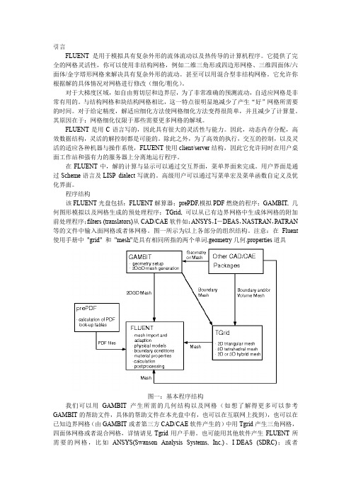
程序结构该FLUENT光盘包括：FLUENT解算器；prePDF,模拟PDF燃烧的程序；GAMBIT, 几何图形模拟以及网格生成的预处理程序；TGrid, 可以从已有边界网格中生成体网格的附加前处理程序；filters (translators)从CAD/CAE软件如：ANSYS，I－DEAS，NASTRAN，PATRAN 等的文件中输入面网格或者体网格。

图一所示为以上各部分的组织结构。

注意：在Fluent 使用手册中"grid" 和"mesh"是具有相同所指的两个单词.geometry几何.properties道具图一：基本程序结构我们可以用GAMBIT产生所需的几何结构以及网格（如想了解得更多可以参考GAMBIT的帮助文件，具体的帮助文件在本光盘中有，也可以在互联网上找到），也可以在已知边界网格（由GAMBIT或者第三方CAD/CAE软件产生的）中用Tgrid产生三角网格，四面体网格或者混合网格，详情请见Tgrid用户手册。

基于fluent的阻力计算(流体力学公式大全)

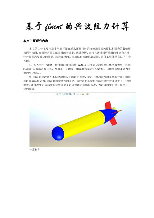
基于fluent的兴波阻力计算本文主要研究内容本文的工作主要涉及小型航行器在近水面航行时的绕流场及兴波模拟和阻力的数值模拟两个方面。

在阅读大量文献资料的基础上，通过分析、比较上述领域所采用的理论和方法，针对目前需要解决的问题，选择合理的方法加以有机地综合运用。

具体工作体现在以下几个方面：1．本人利用FLUENT软件的前处理软件GAMBIT自主建立简单回转体潜器模型，利用FLUENT求解器进行计算，得出在不同潜深下潜器直线航行的绕流场、自由面形状及阻力系数的变化情况。

2．通过对比潜器在不同潜深情况下的阻力系数，论证了增加近水面小型航行器的深度可以有效降低阻力。

通过对模型型线的改动，为近水面小型航行器的型线设计提供了一定的参考。

通过改变附体形状和位置计算了附体对阻力的影响程度，为附体的优化设计提供了一定的依据。

计算模型航行器粘性流场的数值计算理论水动力计算数学模型的建立根据流体运动时所遵循的物理定律，基于合理假设（连续介质假设）用定量的数学关系式表达其运动规律，这些表达式成为流体运动的数学模型，它们是对流体运动的一种定量模型化，称为流体运动控制方程组。

根据控制方程组，结合预先给定的初始条件和边界条件，就可以求解反映流体运动的变量值，从而实现对流体运动的数值模拟预报，形成分析报告。

基于连续介质假设的流体力学中流体运动必须满足要遵循的物理定律:1) 质量守恒定律2）动量守恒定律3）能量守恒定律4）组分质量守恒方程针对具体研究的问题，有选择的满足上述四个定律。

船体的粘性不可压缩绕流运动，如果不考虑水温对水物理性质的影响，水的密度和分子粘性系数都是常数，同时没有能量的转换，就仅仅需要满足质量守恒定律、动量守恒定律。

在满足这些定律下所建立的数学模型称为Navier-Stokes方程。

另外，自由液面的存在也需要建立合适的数学模型。

本文是利用FLUENT 进行数值模拟，而软件里面关于自由液面模拟是用界面追踪方法的一种－流体体积法（VOF）,基于该方法所建立的数学模型称为流体体积分数方程。

FLUENT算例 (3)三维圆管紊流流动状况的数值模拟分析

三维圆管紊流流动状况的数值模拟分析在工程和生活中，圆管内的流动是最常见也是最简单的一种流动，圆管流动有层流和紊流两种流动状况。

层流，即液体质点作有序的线状运动，彼此互不混掺的流动；紊流，即液体质点流动的轨迹极为紊乱，质点相互掺混、碰撞的流动。

雷诺数是判别流体流动状态的准则数。

本研究用CFD 软件来模拟研究三维圆管的紊流流动状况，主要对流速分布和压强分布作出分析。

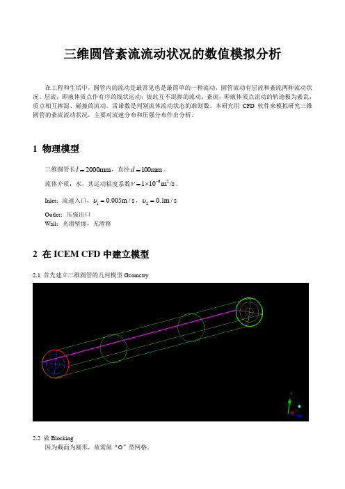
1 物理模型三维圆管长2000mm l =，直径100mm d =。

流体介质：水，其运动粘度系数62110m /s ν-=⨯。

Inlet ：流速入口，10.005m /s υ=，20.1m /s υ= Outlet ：压强出口Wall ：光滑壁面，无滑移2 在ICEM CFD 中建立模型2.1 首先建立三维圆管的几何模型Geometry2.2 做Blocking因为截面为圆形，故需做“O ”型网格。

2.3 划分网格mesh注意检查网格质量。

在未加密的情况下，网格质量不是很好，如下图因管流存在边界层，故需对边界进行加密，网格质量有所提升，如下图2.4 生成非结构化网格，输出fluent.msh等相关文件3 数值模拟原理紊流流动当以水流以流速20.1m /s υ=，从Inlet 方向流入圆管，可计算出雷诺数10000υdRe ν==，故圆管内流动为紊流。

假设水的粘性为常数（运动粘度系数62110m /s ν-=⨯）、不可压流体，圆管光滑，则流动的控制方程如下：①质量守恒方程：()()()0u v w t x y zρρρρ∂∂∂∂+++=∂∂∂∂ (0-1)②动量守恒方程：2()()()()()()()()()()[]u uu uv uw u u ut x y z x x y y z z u u v u w p x y z xρρρρμμμρρρ∂∂∂∂∂∂∂∂∂∂+++=++∂∂∂∂∂∂∂∂∂∂'''''∂∂∂∂+----∂∂∂∂ (0-2)2()()()()()()()()()()[]v vu vv vw v v v t x y z x x y y z z u v v v w px y z yρρρρμμμρρρ∂∂∂∂∂∂∂∂∂∂+++=++∂∂∂∂∂∂∂∂∂∂'''''∂∂∂∂+----∂∂∂∂ (0-3)2()()()()()()()()()()[]w wu wv ww w w w t x y z x x y y z z u w v w w px y z zρρρρμμμρρρ∂∂∂∂∂∂∂∂∂∂+++=++∂∂∂∂∂∂∂∂∂∂'''''∂∂∂∂+----∂∂∂∂ (0-4)③湍动能方程：()()()()[())][())][())]t t k k t k k k ku kv kw k k t x y z x x y yk G z zμμρρρρμμσσμμρεσ∂∂∂∂∂∂∂∂+++=+++∂∂∂∂∂∂∂∂∂∂+++-∂∂ (0-5)④湍能耗散率方程：212()()()()[())][())][())]t t k k t k k u v w t x y z x x y y C G C z z k kεεμμρερερερεεεμμσσμεεεμρσ∂∂∂∂∂∂∂∂+++=+++∂∂∂∂∂∂∂∂∂∂+++-∂∂ (0-6)式中，ρ为密度，u 、ν、w 是流速矢量在x 、y 和z 方向的分量，p 为流体微元体上的压强。

FLUENT实例5个(转自他人)

前言为了使学生尽快熟悉计算流体软件FLUENT以及更好的掌握计算流体力学的计算模型，本书编制了几个简单的模型，包括了组分燃烧、管内流动、换热和房间温度场四个方面的内容。

其中概括了二维和三维的模型，描述详细，可根据步骤建模、划分网格和计算以及后处理。

本书不可能面面具到并进行详细讲解，但相信读者通过本书的学习，一定能领会其中的技巧。

目录前言﹍﹍﹍﹍﹍﹍﹍﹍﹍﹍﹍﹍﹍﹍﹍﹍﹍﹍﹍﹍﹍﹍﹍﹍﹍1 燃烧器内甲烷和空气的燃烧﹍﹍﹍﹍﹍﹍﹍﹍﹍﹍﹍﹍﹍﹍﹍3 管内层流流动数值计算﹍﹍﹍﹍﹍﹍﹍﹍﹍﹍﹍﹍﹍﹍﹍﹍ 38 蒸汽喷射器内的传热模拟﹍﹍﹍﹍﹍﹍﹍﹍﹍﹍﹍﹍﹍﹍﹍ 52 组分传输与气体燃烧算例﹍﹍﹍﹍﹍﹍﹍﹍﹍﹍﹍﹍﹍﹍﹍ 75 空调房间温度场的模拟﹍﹍﹍﹍﹍﹍﹍﹍﹍﹍﹍﹍﹍﹍﹍﹍102燃烧器内甲烷和空气的燃烧问题描述这个问题在图1中以图解的形式表示出来。

此几何体包括一个简化的向燃烧腔加料的燃料喷嘴，由于几何结构对称可以仅做出燃烧室几何体的1/4模型。

喷嘴包括两个同心管，其直径分别是4个单位和10个单位，燃烧室的边缘与喷嘴下的壁面融合在一起。

图1：问题图示一、利用GAMBIT建立计算模型启动GAMBIT。

第一步：选择一个解算器选择用于进行CFD计算的求解器。

操作：Solver -> FLUENT5/6第二步：生成两个圆柱体1、生成一个柱体以形成燃烧室操作：GEOMETRY-> VOLUME-> CREATE VOLUMER打开Create Real Cylinder 窗口，如图2所示a) 在柱体的Height 中键入值1.2。

b) 在柱体的Radius 1 中键入值0.4。

Radius 2的文本键入框可留为空白，GAMBIT 将默认设定为Radius 1值相等。

c) 选择Positive Z （默认）作为Axis Location 。

d) 点击Apply 按钮。

2、按照上述步骤以生成一个Height =2，Radius 1 =1并以positive z 为轴的柱体。

一种基于ANSYS和FLUENT的海洋立管的涡激响应分析方法

文章编号:1001-4500(2007)04-0032-05一种基于AN SYS和FLU ENT的海洋立管的涡激响应分析方法任大朋,黄一,刘刚(大连理工大学,大连116023)摘要:目前提出了一种包括CFD流场分析和结构有限元分析的迭代方法用于模拟海洋立管的涡激振动。

在迭代过程中,依次对流场和立管进行分析。

在分析过程中把直接导致涡激振动的水动力载荷由流场传递到立管,该水动力载荷包括周期性的升力和阻力。

然后把立管的振动定义为一个函数,用来描述下一步计算中流场中立管边界的运动。

计算过程中,采用F LUEN T(6.1.22版本)分析流场和A NSY S(8.1版本)计算立管的涡激响应。

关键词:立管;涡激振动;算法中图分类号:T P399 文献标识码:A当波浪和海流流经立管时,在一定的流速条件下,在立管两侧交替形成一对固定对称的旋涡,该旋涡引起的周期性阻力可使圆柱体在来流方向发生振动,即所谓线内振动或纵向振动;随着流速的增大,在立管两侧交替形成强烈的旋涡,旋涡脱落会对立管产生一个周期性的可变力,使得立管在与流向垂直的方向上发生横向振动,又称为垂向振动,与此同时,旋涡的产生和泄放,还会对柱体产生顺流方向的曳力,也是周期性的力,但它并不改变方向,只是周期性的增减而已,这会引起立管的纵向振动。

结构的振动反过来又对流场产生影响,使旋涡增强,阻力增加,在一般情况下,纵向振动比横向振动幅值约小一个数量级,频率约是其两倍。

近年来的大量试验和研究表明,立管的横向振动和纵向振动都对整个立管系统的疲劳破坏有不可忽略的贡献。

对于近海勘探和开采的深水立管系统,由涡激振动导致的应力是其中一个重要的疲劳载荷。

它对深水立管系统的影响主要有: 由于扩大拖曳而增大变形;由于涡激振动引起的动力应力而导致结构疲劳损伤。

涡激振动分析结果可用于评定立管的强度和疲劳积累。

因此,研究深水立管的涡激振动,是深水立管的疲劳、断裂及可靠性评估研究中的重要部分。

fluent湍流模型技巧

湍流模型目前计算流体力学常用的湍流的数值模拟方法主要有以下三种：一1I（接模拟（directnumericalsimulation,DNS）直接数值模拟（DNS）特点在湍流尺度下的网格尺寸内不引入任何封闭模型的前提下对Navier-Stokes 方程直接求解。

这种方法能对湍流流动中最小尺度涡进行求解，要对高度复杂的湍流运动进行直接的数值计算，必须采用很小的时间与空间步长，才能分辨出湍流中详细的空间结构及变化剧烈的时间特性。

基于这个原因，DNS目前仅限于相对低的雷诺数中湍流流动模型。

另外，利用DNS模型对湍流运动进行直接的数值模拟对计算工具有很高的要求，计算机的内存及计算速度要非常的高，目前DNS模型还无法应用于工程数值计算，还不能解决工程实际问题。

一大涡模拟（largeeddysimulation,LES）大涡模拟（LES）是基于网格尺度封闭模型及对大尺度涡进行直接求解N-S方程，其网格尺度比湍流尺度大,=可以模拟湍流发展过程的一些细节但其计算量仍很大,=也仅用于比较=简单的剪切流运动及管流。

大涡模拟的基础是：湍流的脉动与混合主要是由大尺度的涡造成的，大尺度涡是高度的非各向同性，而且随流动的情形而异。

大尺度的涡通过相互作用把能量传递给小尺度的涡，而小尺度的涡旋主要起到耗散能量的作用，几乎是各向同性的。

这些对涡旋的认识基础就导致了大涡模拟方法的产生。

Les大涡模拟采用非稳态的N-S方程直接模拟大尺度涡，但不计算小尺度涡，小涡对大涡的影响通过近似的模拟来考虑，这种影响称为亚格子Reynolds应力模型。

大多数亚格子Reynolds模型都是将湍流脉动所造成的影响用一个湍流粘性系数，既粘涡性来描述。

LES对计算机的容量和CPU的要求虽然仍然很高，但是远远低于DNS方法对计算机的要求，因而近年来的研究与应用日趋广泛。

一।应用Reynolds时均方程（Reynolds-averagingequations）的模拟方法许多流体力学的研究和数值模拟的结果表明，可用于工程上现实可行的湍流模拟方法仍然是基于求解Reynolds时均方程及关联量输运方程的湍流模拟方法，即湍流的统观模拟方法。

FLUENT中文全教程_部分12

粘性模型面板来激活。

增加的项可能出现在能量方程中，这取决于你所用的物理模型。

想知道细节可以看11.2.1章节。

对于标准和带旋流修正k－e模型热传导系数为：这里a由方程10.4-9算出，a0＝1/Pr＝k/uc p。

实际上a随着umol/ueff_而变就像在方程10.4-9中，这是RNG模型的优点。

这和试验相吻合：湍流能量普朗特数随着分子Prandtl数和湍流变化。

方程10.4-9的有效范围很广，从分子Prandtl数在液体的10-2到石蜡的103，这样使得热传导可以在低雷诺数中计算。

方程10.4-9平稳的预测了有效的湍流能量普朗特数，从粘性占主要地位的区域的a＝1/Pr到完全湍流区域的a＝1.393。

对于湍流物质交换同样对待，对于标准和带旋流修正k－e模型，默认的Schmidt数是0.7。

可以在粘性模型面板中改变。

对于RNG模型，有效的湍流物质交换扩散率用一种热交换的计算方法计算。

方程10.4-9的a0＝1/Sc，这里Sc是molecular数。

10.5 标准和SST k-ω模型这一章讲述标准和SST k-ω模型。

俩种模型有相似的形式，有方程k和ω。

SST和标准模型的不同之处是·从边界层内部的标准k-ω模型到边界层外部的高雷诺数的k－e模型的逐渐转变·考虑到湍流剪应力的影响修改了湍流粘性公式10.5 标准k-ω模型标准k-ω模型是一种经验模型，是基于湍流能量方程和扩散速率方程。

由于k-ω模型已经修改多年，k方程和ω方程都增加了项，这样增加了模型的精度标准k-ω模型的方程在方程中，G k是由层流速度梯度而产生的湍流动能。

Gω是由ω方程产生的。

T k和Tω表明了k 和ω的扩散率。

Y k和Yω由于扩散产生的湍流。

，所有的上面提及的项下面都有介绍。

S k和S e 是用户定义的。

模型扩散的影响对k-ω模型，扩散的影响：这里σk和σω是k、ω方程的湍流能量普朗特数。

湍流粘度u t:低雷诺数修正系数a*使得湍流粘度产生低雷诺数修正。

fluent湍流模型技巧

湍流模型目前计算流体力学常用的湍流的数值模拟方法主要有以下三种：⌝直接模拟（direct numerical simulation, DNS）直接数值模拟（DNS）特点在湍流尺度下的网格尺寸内不引入任何封闭模型的前提下对Navier-Stokes方程直接求解。

基于这个原因，DNS目前仅限于相对低的雷诺数中湍流流动模型。

⌝大涡模拟(large eddy simulation, LES)大涡模拟（LES）是基于网格尺度封闭模型及对大尺度涡进行直接求解N-S方程，其网格尺度比湍流尺度大，可以模拟湍流发展过程的一些细节，但其计算量仍很大，也仅用于比较简单的剪切流运动及管流。

大涡模拟的基础是：湍流的脉动与混合主要是由大尺度的涡造成的，大尺度涡是高度的非各向同性，而且随流动的情形而异。

大尺度的涡通过相互作用把能量传递给小尺度的涡，而小尺度的涡旋主要起到耗散能量的作用，几乎是各向同性的。

这些对涡旋的认识基础就导致了大涡模拟方法的产生。

大多数亚格子Reynolds模型都是将湍流脉动所造成的影响用一个湍流粘性系数，既粘涡性来描述。

LES对计算机的容量和CPU的要求虽然仍然很高，但是远远低于DNS方法对计算机的要求，因而近年来的研究与应用日趋广泛。

⌝应用Reynolds时均方程(Reynolds-averaging equations)的模拟方法许多流体力学的研究和数值模拟的结果表明，可用于工程上现实可行的湍流模拟方法仍然是基于求解Reynolds时均方程及关联量输运方程的湍流模拟方法，即湍流的统观模拟方法。

大涡模拟的fluent算例

Introduction:This tutorial demonstrates how to model the2D turbu-lentﬂow across a circular cylinder using LES(Large Eddy Simula-tion),and computeﬂow-induced noise(aero-noise)using FLUENT’s acoustics model.In this tutorial you will learn how to:•Perform2D Large Eddy Simulation(LES)•Set parameters for an aero-noise calculation•Save surface pressure data for an aero-noise calculation•Calculate aero-noise quantities•Postprocess an aero-noise solutionPrerequisites:This tutorial assumes that you are familiar with the menu structure in FLUENT,and that you have solved or read Tu-torial1.Some steps in the setup and solution procedure will not be shown explicitly.Problem Description:The problem considers turbulent airﬂow over a2D circular cylinder at a free stream velocity U of69.19m/s.The cylinder diameter D is1.9cm.The Reynolds number based on theﬂow parameters is about90000.The computational do-main(Figure3.0.1)extends5D upstream and20D downstream of the cylinder,and5D on both sides of it.If the computational domain is not taken wide enough on the downstream side,so that no reversedﬂow occurs,the accuracy of the aero-noise prediction may be aﬀected.The rule of thumb is to take at least20D on the downstream side of the obstacle.c Fluent Inc.June20,20023-1Aero-Noise Prediction of Flow Across a Circular CylinderAero-Noise Prediction of Flow Across a Circular Cylindernoise.msh.File−→Read−→Case...As FLUENT reads the gridﬁle,it will report its progress in the console window.2.Check the grid.Grid−→CheckFLUENT will perform various checks on the mesh and will report the progress in the console window.Pay particular attention to the reported minimum volume.Make sure this is a positive number.3.Scale the grid.Grid−→Scale...(a)Under Units Conversion,select cm in the Grid Was Created indrop-down list.(b)Click on Scale.4.Display the grid.Display−→Grid...(a)Display the grid with the default settings(Figure3.0.2).(b)Use the middle mouse button to zoom in on the image so youcan see the mesh near the cylinder(Figure3.0.3).Quadrilateral cells are used for this LES simulation becausethey generate less numerical diﬀusion than triangular cells.Cell size should also be small enough to make numerical dif-fusion much smaller than subgrid scale turbulence viscosity.Extra:You can use the right mouse button to check which zone number corresponds to each boundary.If you clickthe right mouse button on one of the boundaries in thegraphics window,its zone number,name,and type will beprinted in the FLUENT console window.This feature is c Fluent Inc.June20,20023-3Aero-Noise Prediction of Flow Across a Circular CylinderAero-Noise Prediction of Flow Across a Circular CylinderAero-Noise Prediction of Flow Across a Circular CylinderAero-Noise Prediction of Flow Across a Circular CylinderAero-Noise Prediction of Flow Across a Circular CylinderAero-Noise Prediction of Flow Across a Circular CylinderAero-Noise Prediction of Flow Across a Circular CylinderAero-Noise Prediction of Flow Across a Circular CylinderAero-Noise Prediction of Flow Across a Circular CylinderAero-Noise Prediction of Flow Across a Circular CylinderAero-Noise Prediction of Flow Across a Circular Cylindernoise1.cas/dat).File−→Write−→Case&data...You can skip items9-12to avoid the time-consuming calculationsnecessary to get the“dynamically steady state”ﬂowﬁeld.Instead,you can read the corresponding case and dataﬁles(cylnoise1.cas/dat).See Chapter28of the User’s Guide for more information on using3-14c Fluent Inc.June20,2002Aero-Noise Prediction of Flow Across a Circular CylinderAero-Noise Prediction of Flow Across a Circular Cylindernoise2.cas/dat).File−→Write−→Case&Data...Step7:Aero-Noise Calculation1.Save surface pressure variation data.(a)Set up the schemeﬁle and user-deﬁned functions(UDFs)foraero-noise calculation.i.Read the schemeﬁle,normally located in the lib directory,to create the Acoustic-Parameters panel.File−→Read−→Scheme...ii.Select acousticAero-Noise Prediction of Flow Across a Circular CylinderAero-Noise Prediction of Flow Across a Circular Cylindernoisenoise noisenoisenoise whole for the File Name to Read Surface Pressure.FLUENT’s aero-noise calculation module operates on asingleﬁle of surface pressure data at a time.If the surfacepressure data is saved in separateﬁles,you may want toconcatenate them into one singleﬁle.3-18c Fluent Inc.June20,2002Aero-Noise Prediction of Flow Across a Circular Cylinderacousticpowerpower db.xy for the File Name to Power Spectrum in dB Unit.(c)Changeﬁle name for the surface monitor.Solve−→Monitor−→Surface...i.Click on Deﬁne next to monitor-1ii.In the Deﬁne Surface Monitor panel,change the name of the monitor from monitor-point-behind-pres1-1.outto monitor-point-behind-pres4-1.out.(d)Save case and dataﬁles(cylnoise4.cas/dat).File−→Write−→Case&Data...(g)Exit FLUENTFile−→ExitIt is necessary to exit parallel FLUENT because the followingaero-noise calculation is performed with an Execute On De-mand UDF,which can only be used in the serial version ofthe solver.2.Calculate aero-noise(a)Start the serial version of FLUENT.c Fluent Inc.June20,20023-19Aero-Noise Prediction of Flow Across a Circular Cylinderpar.scm).File−→Read−→Scheme...(c)Read case and dataﬁles(cylnoise noise noise noise noise noisenoise whole.If you did not perform the calculation to write theﬁles thatwill be used in this step,you can continue by using the corre-spondingﬁles provided in the documentation CD.(e)Use the Execute On Demand UDF to perform the aero-noisecalculation.Deﬁne−→User-Deﬁned−→Execute On Demand...(f)Select the cal-sound UDF and click Execute.Note:There is a limit to the minimum number of time steps ac-cording to the sound calculation scheme.The minimum num-ber of time steps needs to be larger than n=T/dt,where Tis the propagation time through a distance L,roughly equalto the length scale of the sound generating wall,and dt is thetime step size applied in the unsteady calculation.If the givennumber of time steps for cal-sound is smaller than the requiredminimum number,a warning will be printed on FLUENT’sconsole window,along with the indication of the minimumnumber<n>of time steps requiredWarning:Number of Time Steps of The Input Surface Data Must be Larger Than:<n>.3-20c Fluent Inc.June20,2002Aero-Noise Prediction of Flow Across a Circular Cylinder1.69e+021.52e+021.35e+021.19e+021.02e+028.49e+016.80e+015.12e+013.43e+011.75e+016.49e-01Figure3.0.7:Velocity Vectors2.Display contours of static pressure at the current time step(Fig-ure3.0.8).Display−→Contours...3.Inspect the Sound Pressure Level(SPL)value.The the value ofsound intensity in units of W/m2and its alternative expression in dB are printed in the FLUENT console window after the execution of the cal-sound UDF,and areIntensity=4.060634e+00(W/m2)SPL=1.261719e+02(dB)c Fluent Inc.June20,20023-21Aero-Noise Prediction of Flow Across a Circular Cylinder3.91e+031.78e+03-3.56e+02-2.49e+03-4.62e+03-6.75e+03-8.89e+03-1.10e+04-1.32e+04-1.53e+04-1.74e+04Figure3.0.8:Static Pressure Contours4.Plot Acoustic Pressure variation(Figure3.0.9).Plot−→File...(a)Click on Add.(b)Select theﬁle cyl pres.xy and click OK.Remember to delete theﬁles you do not want to display from theFiles list.5.Plot Power Spectrum of sound pressure(Figure3.0.10).(a)Power Spectrum in units of P a2.Plot−→File...i.Click on Add.ii.Select theﬁle cyl spectrum.xy and click OK.Figure3.0.10shows a frequency range of0−2000Hz,withmajor and minor rules turned on.From thisﬁgure it can be 3-22c Fluent Inc.June20,2002Aero-Noise Prediction of Flow Across a Circular CylinderAero-Noise Prediction of Flow Across a Circular Cylinderpower db.xy and click OK .Frequency (Hz)5.00e+016.00e+017.00e+018.00e+019.00e+011.00e+021.10e+021.20e+0201e+032e+033e+034e+035e+036e+037e+038e+039e+031e+04Power Spectrum (dB)Figure 3.0.11:Plot of Power Spectrum of Sound Pressure.Figure 3.0.11shows a frequency range of 0−10kHz .6.Inspect Surface Dipole Strength.(a)Display contours of Surface Dipole Strength on surface cylin-der (Figure 3.0.12).Display −→Contours...i.In the Contours Of drop-down lists,select User-DeﬁnedMemory and udm-0.ii.Turn oﬀNode Values .3-24cFluent Inc.June 20,2002Aero-Noise Prediction of Flow Across a Circular Cylinder4.13e+053.72e+053.31e+052.89e+052.48e+052.07e+051.65e+051.24e+058.25e+044.12e+04-1.94e+02Figure3.0.12:Contour of Surface Dipole Strengthiii.Click on Display.The value of Surface Dipole Strength for each cell face is storedfor the center of the face on the cylinder wall.Surface DipoleStrength is the distribution of unit area contribution on thesound generating surface to the intensity of sound measuredat the observer’s location.(b)Plot Surface Dipole Strength(udm-0)on surface cylinder(Fig-ure3.0.13).Plot−→XY Plot...Figure3.0.13shows Surface Dipole Strength distribution onboth the upper and lower half cylinder faces.Extra:Once theﬂow simulation reaches a“dynamically steady state”, the accuracy for predicting Sound Pressure Level(SPL)and Power Spectrum is usually dependent on the number of time steps used.LES requires a mesh size as small as the length scale of eddies in the inertial sub-range.The corresponding time step size is calcu-c Fluent Inc.June20,20023-25Aero-Noise Prediction of Flow Across a Circular CylindercylinderFigure3.0.13:Plot of Surface Dipole Strengthlated by dt=Cdx/U,where C is the Courant number,and thus isvery small compared with the period T of the dominating acousticwave component(i.e.that corresponding to the frequency of thehighest peak in the power spectrum).For an accurate aero-noiseprediction,at least10periods of the dominating wave componentare required for sampling.The number of time steps for this re-quirement can be roughly estimated for theﬂow over the cylinder.In a certain Reynolds number range(roughly Re<50000),theStrouhal number(St=fD/U)for the dominating frequency f isabout0.2.Therefore,the period is T=D/0.2/U.From the aboveequations,the number of time steps for each period can be calcu-lated as N=T/dt=5/CD/dx.In LES,the ratio between thedomain scale D and the typical cell size dx can easily be50-100.As an example,if C is taken as order of1,N can be as high as250-500for each period.For40periods,10000-20000time stepsmay be required.Summary:This tutorial demonstrated how to set up and calculate an aero-noise problem for theﬂow around a cylinder,using the2D LES 3-26c Fluent Inc.June20,2002Aero-Noise Prediction of Flow Across a Circular CylinderAero-Noise Prediction of Flow Across a Circular Cylinder。

Fluent模型使用技巧

Fluent模型使⽤技巧1.多相流动模式我们可以根据下⾯的原则对多相流分成四类：⽓-液或者液-液两相流：o⽓泡流动：连续流体中的⽓泡或者液泡。

o液滴流动：连续⽓体中的离散流体液滴。

o活塞流动:在连续流体中的⼤的⽓泡o分层⾃由⾯流动：由明显的分界⾯隔开的⾮混合流体流动。

⽓-固两相流：o充满粒⼦的流动：连续⽓体流动中有离散的固体粒⼦。

o⽓动输运：流动模式依赖诸如固体载荷、雷诺数和粒⼦属性等因素。

最典型的模式有沙⼦的流动，泥浆流，填充床，以及各向同性流。

o流化床：由⼀个盛有粒⼦的竖直圆筒构成，⽓体从⼀个分散器导⼊筒内。

从床底不断充⼊的⽓体使得颗粒得以悬浮。

改变⽓体的流量，就会有⽓泡不断的出现并穿过整个容器，从⽽使得颗粒在床内得到充分混合。

液-固两相流o泥浆流：流体中的颗粒输运。

液-固两相流的基本特征不同于液体中固体颗粒的流动。

在泥浆流中，Stokes数通常⼩于1。

当Stokes数⼤于1时，流动成为流化（fluidization）了的液-固流动。

o⽔⼒运输:在连续流体中密布着固体颗粒o沉降运动:在有⼀定⾼度的成有液体的容器内，初始时刻均匀散布着颗粒物质。

随后，流体将会分层，在容器底部因为颗粒的不断沉降并堆积形成了淤积层，在顶部出现了澄清层，⾥⾯没有颗粒物质，在中间则是沉降层，那⾥的粒⼦仍然在沉降。

在澄清层和沉降层中间，是⼀个清晰可辨的交界⾯。

三相流(上⾯各种情况的组合)各流动模式对应的例⼦如下：⽓泡流例⼦：抽吸，通风，空⽓泵，⽓⽳，蒸发，浮选，洗刷液滴流例⼦：抽吸，喷雾，燃烧室，低温泵，⼲燥机，蒸发，⽓冷，刷洗?活塞流例⼦：管道或容器内有⼤尺度⽓泡的流动分层⾃由⾯流动例⼦：分离器中的晃动，核反应装置中的沸腾和冷凝粒⼦负载流动例⼦：旋风分离器，空⽓分类器，洗尘器，环境尘埃流动风⼒输运例⼦：⽔泥、⾕粒和⾦属粉末的输运流化床例⼦：流化床反应器，循环流化床泥浆流例⼦:泥浆输运，矿物处理⽔⼒输运例⼦：矿物处理，⽣物医学及物理化学中的流体系统沉降例⼦：矿物处理2.多相流模型FLUENT中描述两相流的两种⽅法:欧拉⼀欧拉法和欧拉⼀拉格朗⽇法，后⾯分别简称欧拉法和拉格朗⽇法。

大涡模拟

大涡模拟,英文简称LES(Large eddy simulation),是近几十年才发展起来的一个流体力学中重要的数值模拟研究方法。

它区别于直接数值模拟(DNS)和雷诺平均(RANS)方法。

其基本思想是通过精确求解某个尺度以上所有湍流尺度的运动，从而能够捕捉到RANS方法所无能为力的许多非稳态，非平衡过程中出现的大尺度效应和拟序结构，同时又克服了直接数值模拟由于需要求解所有湍流尺度而带来的巨大计算开销的问题，因而被认为是最具有潜力的湍流数值模拟发展方向。

由于计算耗费依然很大，目前大涡模拟还无法在工程上广泛应用，但是大涡模拟技术对于研究许多流动机理问题提供了更为可靠的手段，可为流动控制提供理论基础，并可为工程上广泛应用的RANS方法改进提供指导。

大涡模拟方法其主要思想是大涡结构（又称拟序结构）受流场影响较大，小尺度涡则可以认为是各向同性的，因而可以将大涡计算与小涡计算分开处理，并用统一的模型计算小涡。

在这个思想下，大涡模拟通过滤波处理，首先将小于某个尺度的旋涡从流场中过滤掉，只计算大涡，然后通过求解附加方程得到小涡的解。

过滤尺度一般就取为网格尺度。

显然这种方法比直接求解RANS 方程和DNS 方程效率更高，消耗系统资源更少，但却比湍流模型方法更精确。

大涡模拟的基本操作就是低通滤波。

一个LES滤波器可以被用在时空场Φ（x,t）中实现时间滤波或空间滤波或时空滤波扬州大学大涡模拟理论及应用紊流力学大涡模拟理论及应用一、概述实际水利工程中的水流流动几乎都是湍流。

湍流是空间上不规则和时间上无秩序的一种非线性的流体运动，这种运动表现出非常复杂的流动状态，是流体力学中有名的难题。

100 多年来无数科学家投身到它的研究当中，从1883 年Reynolds 开始的层流过渡到湍流的著名圆管实验到现在，对湍流的基础理论研究呈现出多个分支，其主要方向有：湍流稳定性理沦、湍流统计理论、湍流模式理论、湍流实验、切变湍流的逆序结构、湍流的大涡模拟和湍流的直接数值模拟。

紊流计算理论公式

湍流量的指定方法湍流强度I定义为相对于平均速度u_avg的脉动速度u^'的均方根。

小于或等于1%的湍流强度通常被认为低强度湍流，大于10%被认为是高强度湍流。

从外界，测量数据的入口边界，你可以很好的估计湍流强度。

例如：如果你模拟风洞试验，自由流的湍流强度通常可以从风洞指标中得到。

在现代低湍流风洞中自由流湍流强度通常低到0.05%。

.对于内部流动，入口的湍流强度完全依赖于上游流动的历史，如果上游流动没有完全发展或者没有被扰动，你就可以使用低湍流强度。

如果流动完全发展，湍流强度可能就达到了百分之几。

完全发展的管流的核心的湍流强度可以用下面的经验公式计算：例如，在雷诺数为50000是湍流强度为4%湍流尺度l是和携带湍流能量的大涡的尺度有关的物理量。

在完全发展的管流中，l被管道的尺寸所限制，因为大涡不能大于管道的尺寸。

L和管的物理尺寸之间的计算关系如下：l07L=.0其中L为管道的相关尺寸。

因子0.07是基于完全发展湍流流动混合长度的最大值的，对于非圆形截面的管道，你可以用水力学直径取代L。

如果湍流的产生是由于管道中的障碍物等特征，你最好用该特征长度作为湍流长度L而不是用管道尺寸。

注意：公式Ll07=并不是适用于所有的情况。

它只是在大多.0数情况下得很好的近似。

对于特定流动，选择L和l的原则如下：对于完全发展的内部流动，选择强度和水力学直径指定方法，并在水力学直径流场中指定L=D_H。

对于旋转叶片的下游流动，穿孔圆盘等，选择强度和水力学直径指定方法，并在水力学直径流场中指定流动的特征长度为L 对于壁面限制的流动，入口流动包含了湍流边界层。

选择湍流强度和长度尺度方法并使用边界层厚度d_99来计算湍流长度尺度l，在湍流长度尺度流场中输入l=0.4d_99这个值湍流粘性比m_t/m直接与湍流雷诺数成比例(Re_t?k^2/(e n))。

Re_t在高湍流数的边界层，剪切层和完全发展的管流中是较大的(100到1000)。

FLUENT软件实际操作

求解技术（Solve）Solve>Controls>Solution…计算格式的选择一阶迎风格式：适用于流动方向与网格方向基本一致，结构化网格。

具有稳定性高，计算速度快的优点。

在网格方向与流动方向不一致时，产生的数值误差比较大。

二阶格式：计算时间比较长，收敛性差。

合适的计算方式：在计算开始时先用一阶格式进行计算以获得一个相对粗糙的解，在计算收敛后再用二阶格式完成计算以提高解的精度。

避免二阶格式收敛性差、计算时间长的问题，也避免了一阶格式在复杂流场计算中数值误差大的问题。

QUICK格式：对于结构网格计算旋转流动问题时，计算精度高，但在其它情况下，QUCIK格式的精度与二阶格式相当。

指数律格式：与一阶格式精度基本相同。

中心差分：在LES湍流模型中使用，且应该在网格足够密集、局部Peclet数小于1的情况下使用。

压强插值格式的选择1在彻体力对流场有很大影响的情况下，应该选择彻体力加权（body-force-weighted）格式。

2 在流场中有涡量很大的集中涡、高雷诺数自然对流、高速旋转流、多孔介质，以及流线曲率很大时，应该选择PRESTO!格式。

3 对于可压流，应该使用二阶格式。

4 二阶格式不能用于多孔介质计算和多相流计算中的混合物模型及VOF 模型。

在其他情况下，为了提高精度可以选用二阶格式。

密度插值格式的选择在用分离算法计算单相可压流时，有三种密度插值格式可供选择，即一阶迎风格式、二阶格式和QUICK 格式。

一阶迎风格式具有良好的稳定性，但是在计算带激波的可压流时，会对激波解产生“抹平”作用，因此应该选用二阶格式或QUICK 格式。

在用四边形网格、六面体网格或混合网格计算带激波的流动时，最好使用QUICK 格式计算所有变量。

需要注意的是，在计算可压多项流时，只能用一阶迎风格式计算可压缩相的流动。

Solve>Controls>Solution…Discretization(离散)定义动量、能量、湍流动能等项目，有一阶迎风格式、二阶迎风格式、指数律格式、QUICK格式和中心差分格式（在LES湍流模式计算中），也可以在使用耦合求解器时，定义湍流动能、湍流耗散率等项目，并为这些项目选择一阶迎风格式、二阶迎风格式。