数字图像处理--灰度形态学 (英文)
形态学图像处理MorphologicalImageProcessing

集合间的关系和运算 – 子集: A B { x | x A, x B}
–
–
– –
»集合A中的每一个元素都是集合B的一个元素。 并集: A B { x | x A或x B} »由集合A和集合B中的所有元素组成的集合 交集: A B { x | x A且x B} »由集合A和集合B中所有既属于A也属于B的公共元素 组成的集合。 如果 A B ,则称互斥的或不相容的 c A { x | x A} 补集。A的补集记为 »由所有不属于集合A的元素组成的集合。 差集: A B {w | w A, w B} A Bc »由所有属于集合A但不属于集合B的元素组成的集合。
A B B {[( AB) B)] B}B
第7章 形态学图像处理
第31页
南京工程学院 林忠
例:
开运算与闭运算
(a)有噪声的图像A (b)结构元素B (c)腐蚀图像 (d)A的开运算 (e)开运算的膨胀 (f)开运算的闭运算
第7章 形态学图像处理
第32页
南京工程学院 林忠
7.5 基本的形态学算法
这里X0=p,结构元素为B,结束条件Xk=Xk-1 对多个区域填充时,需要指定对应的初始点
第7章 形态学图像处理
第35页
南京工程学院 林忠
例:
X k ( X k 1 B) Ac
k 1,2,3,
第7章 形态学图像处理
第36页
南京工程学院 林忠
骨架提取 寻找二值图像的细化结构是图像处理的一个基本问 题,骨架便是这样一种细化结构。 设S(A)表示A的骨架,则求图像A的骨架的过程可 以描述为: N S ( A) Sn ( A)
灰阶名词解释

灰阶名词解释一、什么是灰阶?灰阶(Gray Scale)是一种表达图像亮度变化的方式,它使用不同的灰度级别来表示图像中不同区域的亮度。
在灰阶中,亮度的变化由黑到白,总共包含256个灰度级别,即灰阶范围为0到255。
较小的灰度值表示较暗的区域,较大的灰度值表示较亮的区域。
使用灰阶可以有效地表示黑白图像,也可以用于将彩色图像转换为黑白图像。
在灰阶图像中,每个像素点只有一个灰度值。
二、灰阶的应用领域2.1 数字图像处理在数字图像处理中,灰阶是一项非常重要的概念。
通过改变图像中每个像素的灰度值,可以对图像进行增强、去噪、滤波等操作,以达到改善图像质量或提取图像特征的目的。
2.2 图像分割与边缘检测在图像分割与边缘检测领域,灰阶被广泛应用。
通过分析图像中不同区域的灰度值差异,可以将图像分割成不同的区域,或者检测图像中的边缘。
2.3 图像识别与物体检测在图像识别与物体检测中,灰阶可以用于增强图像的对比度,使物体轮廓更加清晰,从而提高图像的识别和检测性能。
2.4 模式识别与机器学习在模式识别与机器学习领域,灰阶图像通常被用作输入数据。
通过灰阶图像中像素点的灰度值,可以提取图像的特征向量,用于模式分类、机器学习等任务。
三、灰阶的特点与优势3.1 简单直观灰阶使用单一的灰度值来表示图像的亮度,使得图像的处理和分析更加直观。
3.2 信息丰富在灰阶图像中,不同的灰度级别对应着不同的亮度值。
通过改变灰度值,可以增强图像的对比度,使得图像中的细节更加明显。
3.3 适用性广泛灰阶不仅适用于黑白图像的处理,还可以通过色彩空间转换将彩色图像转换为灰阶图像,进而进行灰度处理。
3.4 计算效率高由于灰阶图像只有一个通道,相对于彩色图像而言,它的计算量更小,处理速度更快。
四、灰阶的局限性及改进方法4.1 缺失颜色信息灰阶图像只包含亮度信息,无法表达图像中的颜色信息。
在某些应用中,颜色是十分重要的特征,因此灰阶图像可能无法满足需求。
4.2 对比度有限灰阶图像在表示对比度较大的图像时存在局限性。
数字图像处理第四版拉斐尔课后答案

数字图像处理第四版拉斐尔课后答案数字图像处理(美)Rafael C. Gonzalez(拉斐尔·C. 冈萨雷斯),Richard E. Woods(理查德·E. 伍兹)课后习题答案1. 新增了关于精确直⽅图匹配、⼩波、图像变换、有限差分、k均值聚类、超像素、图割、斜率编码的内容。
2. 扩展了关于⾻架、中轴和距离变换的说明,增加了紧致度、圆度和偏⼼率等描述⼦。
3. 新增了哈⾥斯-斯蒂芬斯⾓点探测器及*稳定极值区域的内容。
扫⼀扫⽂末在⾥⾯回复答案+数字图像处理⽴即得到答案4. 重写了关于神经⽹络和深度学习的内容,全⾯介绍了全连接深度神经⽹络,新增了关于深度卷积神经⽹络的内容。
5. 为学⽣和教师提供⽀持包,⽀持包可从本书的配套⽹站下载。
6. 新增了⼏百幅图像、⼏⼗个新图表和上百道新习题。
在数字图像处理领域,本书作为主要教材已有40多年。
第四版是作者在前三版的基础上修订⽽成的,是前三版的发展与延续。
除保留前⼏版的⼤部分内容外,根据读者的反馈,作者对本书进⾏了全⾯修订,融⼊了近年来数字图像处理领域的重要进展,增加了⼏百幅新图像、⼏⼗个新图表和上百道新习题。
全书共12章,即绪论、数字图像基础、灰度变换与空间滤波、频率域滤波、图像复原与重构、⼩波变换和其他图像变换、彩⾊图像处理、图像压缩和⽔印、形态学图像处理、图像分割、特征提取、图像模式分类。
本书的读者对象主要是从事信号与信息处理、通信⼯程、电⼦科学与技术、信息⼯程、⾃动化、计数字图像处理课后答案(美)Rafael C.Gonzalez(拉斐尔·C. 冈萨雷斯),Richard E. Woods(理查德·E. 伍兹)算机科学与技术、地球物理、⽣物⼯程、⽣物医学⼯程、物理、化学、医学、遥感等领域的⼤学教师和科技⼯作者、研究⽣、⼤学本科⾼年级学⽣及⼯程技术⼈员。
Rafael C. Gonzalez: 1965于美国迈阿密⼤学获电⽓⼯程学⼠学位;1967年和1970年于美国佛罗⾥达⼤学盖恩斯维尔分校分别获电⽓⼯程硕⼠学位和博⼠学位。
digital image processing(数字图像处理)
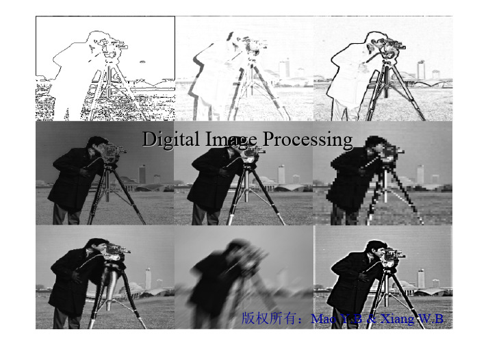
数字图像处理Digital Image Processing版权所有:Mao Y.B & Xiang W.BOutline of Lecture 2•取样与量化•图像灰度直方图•光度学•色度学与彩色模型•人眼视觉特性•噪声与图像质量评价•应用举例采样与量化取样与量化•采样是指将在空间上连续的图像转换成离散的采样点(即像素)集的操作。
由于图像是二维分布的信息,所以采样是在x轴和y轴两个方向上进行。
一般情况下,x轴方向与y轴方向的采样间隔相同取样与量化采样时注意:采样间隔的选取,以及采样保持方式的选取。
•采样间隔太小,则增大数据量;太大,则会发生频率的混叠现象。
•采样保持,一般不做特殊说明都是采用0阶保持的方式,即一个像素的值是其局部区域亮度(颜色)的均值。
采样间隔太大分辨率分辨率是指映射到图像平面上的单个像素的景物元素的尺寸。
单位:像素/英寸,像素/厘米(如:扫描仪的指标300dpi)或者是指要精确测量和再现一定尺寸的图像所必需的像素个数。
单位:像素*像素(如:数码相机指标30万像素(640*480))以多大的采样间隔进行采样为好?取样与量化•点阵采样的数学描述∑∑+∞−∞=+∞−∞=∆−∆−δ=i j )y j y ,x i x ()y ,x (S ∑∑+∞∞−+∞−∞=∆−∆−δ=⋅=j I I P )y j y ,x i x ()y ,x (f )y ,x (S )y ,x (f )y ,x (f ∑∑+∞∞−+∞−∞=∆−∆−δ⋅∆∆=j )y j y ,x i x ()y j ,x i (fc c量化过程取样与量化•量化是将各个像素所含的明暗信息离散化后,用数字来表示。
一般的量化值为整数。
•充分考虑到人眼的识别能力之后,目前非特殊用途的图像均为8bit量化,即用[0 255]描述“从黑到白”。
•量化阶太低,会出现假轮廓现象。
取样与量化量化不足,出现假轮廓取样与量化量化可分为均匀量化和非均匀量化。
数字图像处理论文中英文对照资料外文翻译文献
第 1 页中英文对照资料外文翻译文献原 文To image edge examination algorithm researchAbstract :Digital image processing took a relative quite young discipline,is following the computer technology rapid development, day by day obtains th widespread application.The edge took the image one kind of basic characteristic,in the pattern recognition, the image division, the image intensification as well as the image compression and so on in the domain has a more widesp application.Image edge detection method many and varied, in which based on brightness algorithm, is studies the time to be most long, the theory develo the maturest method, it mainly is through some difference operator, calculates its gradient based on image brightness the change, thus examines the edge, mainlyhas Robert, Laplacian, Sobel, Canny, operators and so on LOG 。
数字图像处理英文原版及翻译
Digital Image Processing and Edge DetectionDigital Image ProcessingInterest in digital image processing methods stems from two principal application areas: improvement of pictorial information for human interpretation; and processing of image data for storage, transmission, and representation for autonomous machine perception.An image may be defined as a two-dimensional function, f(x, y), where x and y are spatial (plane) coordinates, and the amplitude of f at any pair of coordinates (x, y) is called the intensity or gray level of the image at that point. When x, y, and the amplitude values of f are all finite, discrete quantities, we call the image a digital image. The field of digital image processing refers to processing digital images by means of a digital computer. Note that a digital image is composed of a finite number of elements, each of which has a particular location and value. These elements are referred to as picture elements, image elements, pixels, and pixels. Pixel is the term most widely used to denote the elements of a digital image.Vision is the most advanced of our senses, so it is not surprising that images play the single most important role in human perception. However, unlike humans, who are limited to the visual band of the electromagnetic (EM) spec- trum, imaging machines cover almost the entire EM spectrum, ranging from gamma to radio waves. They can operate on images generated by sources that humans are not accustomed to associating with images. These include ultra- sound, electron microscopy, and computer-generated images. Thus, digital image processing encompasses a wide and varied field of applications.There is no general agreement among authors regarding where image processing stops and other related areas, such as image analysis and computer vi- sion, start. Sometimes a distinction is made by defining image processing as a discipline in which both the input and output of a process are images. We believe this to be a limiting and somewhat artificial boundary. For example, under this definition, even the trivial task of computing the average intensity of an image (which yields asingle number) would not be considered an image processing operation. On the other hand, there are fields such as computer vision whose ultimate goal is to use computers to emulate human vision, including learning and being able to make inferences and take actions based on visual inputs. This area itself is a branch of artificial intelligence (AI) whose objective is to emulate human intelligence. The field of AI is in its earliest stages of infancy in terms of development, with progress having been much slower than originally anticipated. The area of image analysis (also called image understanding) is in be- tween image processing and computer vision.There are no clearcut boundaries in the continuum from image processing at one end to computer vision at the other. However, one useful paradigm is to consider three types of computerized processes in this continuum: low-, mid-, and high level processes. Low-level processes involve primitive opera- tions such as image preprocessing to reduce noise, contrast enhancement, and image sharpening. A low-level process is characterized by the fact that both its inputs and outputs are images. Mid-level processing on images involves tasks such as segmentation (partitioning an image into regions or objects), description of those objects to reduce them to a form suitable for computer processing, and classification (recognition) of individual objects. A midlevel process is characterized by the fact that its inputs generally are images, but its outputs are attributes extracted from those images (e.g., edges, contours, and the identity of individual objects). Finally, higher level processing involves “making sense” of an ensemble of recognized objects, as in image analysis, and, at the far end of the continuum, performing the cognitive functions normally associated with vision.Based on the preceding comments, we see that a logical place of overlap between image processing and image analysis is the area of recognition of individual regions or objects in an image. Thus, what we call in this book digital image processing encompasses processes whose inputs and outputs are images and, in addition, encompasses processes that extract attributes from images, up to and including the recognition of individual objects. As a simple illustration to clarify these concepts, consider the area of automated analysis of text. The processes of acquiring an image of the area containing the text, preprocessing that image, extracting(segmenting) the individual characters, describing the characters in a form suitable for computer processing, and recognizing those individual characters are in the scope of what we call digital image processing in this book. Making sense of the content of the page may be viewed as being in the domain of image analysis and even computer vision, depending on the level of complexity implied by the statement “making sense.”As will become evident shortly, digital image processing, as we have defined it, is used successfully in a broad range of areas of exceptional social and economic value.The areas of application of digital image processing are so varied that some form of organization is desirable in attempting to capture the breadth of this field. One of the simplest ways to develop a basic understanding of the extent of image processing applications is to categorize images according to their source (e.g., visual, X-ray, and so on). The principal energy source for images in use today is the electromagnetic energy spectrum. Other important sources of energy include acoustic, ultrasonic, and electronic (in the form of electron beams used in electron microscopy). Synthetic images, used for modeling and visualization, are generated by computer. In this section we discuss briefly how images are generated in these various categories and the areas in which they are applied.Images based on radiation from the EM spectrum are the most familiar, especially images in the X-ray and visual bands of the spectrum. Electromagnet- ic waves can be conceptualized as propagating sinusoidal waves of varying wavelengths, or they can be thought of as a stream of massless particles, each traveling in a wavelike pattern and moving at the speed of light. Each massless particle contains a certain amount (or bundle) of energy. Each bundle of energy is called a photon. If spectral bands are grouped according to energy per photon, we obtain the spectrum shown in fig. below, ranging from gamma rays (highest energy) at one end to radio waves (lowest energy) at the other. The bands are shown shaded to convey the fact that bands of the EM spectrum are not distinct but rather transition smoothly from one to theother.Image acquisition is the first process. Note that acquisition could be as simple as being given an image that is already in digital form. Generally, the image acquisition stage involves preprocessing, such as scaling.Image enhancement is among the simplest and most appealing areas of digital image processing. Basically, the idea behind enhancement techniques is to bring out detail that is obscured, or simply to highlight certain features of interest in an image. A familiar example of enhancement is when we increase the contrast of an image because “it looks better.” It is important to keep in mind that enhancement is a very subjective area of image processing. Image restoration is an area that also deals with improving the appearance of an image. However, unlike enhancement, which is subjective, image restoration is objective, in the sense that restoration techniques tend to be based on mathematical or probabilistic models of image degradation. Enhancement, on the other hand, is based on human subjective preferences regarding what constitutes a “good”enhancement result.Color image processing is an area that has been gaining in importance because of the significant increase in the use of digital images over the Internet. It covers a number of fundamental concepts in color models and basic color processing in a digital domain. Color is used also in later chapters as the basis for extracting features of interest in an image.Wavelets are the foundation for representing images in various degrees of resolution. In particular, this material is used in this book for image data compression and for pyramidal representation, in which images are subdivided successively into smaller regions.Compression, as the name implies, deals with techniques for reducing the storage required to save an image, or the bandwidth required to transmit it.Although storage technology has improved significantly over the past decade, the same cannot be said for transmission capacity. This is true particularly in uses of the Internet, which are characterized by significant pictorial content. Image compression is familiar (perhaps inadvertently) to most users of computers in the form of image , such as the jpg used in the JPEG (Joint Photographic Experts Group) image compression standard.Morphological processing deals with tools for extracting image components that are useful in the representation and description of shape. The material in this chapter begins a transition from processes that output images to processes that output image attributes.Segmentation procedures partition an image into its constituent parts or objects. In general, autonomous segmentation is one of the most difficult tasks in digital image processing. A rugged segmentation procedure brings the process a longway toward successful solution of imaging problems that require objects to be identified individually. On the other hand, weak or erratic segmentation algorithms almost always guarantee eventual failure. In general, the more accurate the segmentation, the more likely recognition is to succeed.Representation and description almost always follow the output of a segmentation stage, which usually is raw pixel data, constituting either the boundary of a region (i.e., the set of pixels separating one image region from another) or all the points in the region itself. In either case, converting the data to a form suitable for computer processing is necessary. The first decision that must be made is whether the data should be represented as a boundary or as a complete region. Boundary representation is appropriate when the focus is on external shape characteristics, such as corners and inflections. Regional representation is appropriate when the focus is on internal properties, such as texture or skeletal shape. In some applications, these representations complement each other. Choosing a representation is only part of the solution for trans- forming raw data into a form suitable for subsequent computer processing. A method must also be specified for describing the data so that features of interest are highlighted. Description, also called feature selection, deals with extracting attributes that result in some quantitative information of interest or are basic for differentiating one class of objects from another.Recognition is the process that assigns a label (e.g., “vehicle”) to an object based on its descriptors. As detailed before, we conclude our coverage of digital image processing with the development of methods for recognition of individual objects.So far we have said nothing about the need for prior knowledge or about the interaction between the knowledge base and the processing modules in Fig 2 above. Knowledge about a problem domain is coded into an image processing system in the form of a knowledge database. This knowledge may be as simple as detailing regions of an image where theinformation of interest is known to be located, thus limiting the search that has to be conducted in seeking that information. The knowledge base also can be quite complex, such as an interrelated list of all major possible defects in a materials inspection problem or an image database containing high-resolution satellite images of a region in connection with change-detection applications. In addition to guiding the operation of each processing module, the knowledge base also controls the interaction between modules. This distinction is made in Fig 2 above by the use of double-headed arrows between the processing modules and the knowledge base, as opposed to single-headed arrows linking the processing modules.Edge detectionEdge detection is a terminology in image processing and computer vision, particularly in the areas of feature detection and feature extraction, to refer to algorithms which aim at identifying points in a digital image at which the image brightness changes sharply or more formally has discontinuities.Although point and line detection certainly are important in any discussion on segmentation,edge detection is by far the most common approach for detecting meaningful discounties in gray level.Although certain literature has considered the detection of ideal step edges, the edges obtained from natural images are usually not at all ideal step edges. Instead they are normally affected by one or several of the following effects:1.focal blur caused by a finite depth-of-field and finite point spread function; 2.penumbral blur caused by shadows created by light sources of non-zero radius; 3.shading at a smooth object edge; 4.local specularities or interreflections in the vicinity of object edges.A typical edge might for instance be the border between a block of red color and a block of yellow. In contrast a line (as can be extracted by a ridge detector) can be a small number of pixels of a different color on an otherwise unchanging background. For a line, there maytherefore usually be one edge on each side of the line.To illustrate why edge detection is not a trivial task, let us consider the problem of detecting edges in the following one-dimensional signal. Here, we may intuitively say that there should be an edge between the 4th and 5th pixels.If the intensity difference were smaller between the 4th and the 5th pixels and if the intensity differences between the adjacent neighbouring pixels were higher, it would not be as easy to say that there should be an edge in the corresponding region. Moreover, one could argue that this case is one in which there are several edges.Hence, to firmly state a specific threshold on how large the intensity change between two neighbouring pixels must be for us to say that there should be an edge between these pixels is not always a simple problem. Indeed, this is one of the reasons why edge detection may be a non-trivial problem unless the objects in the scene are particularly simple and the illumination conditions can be well controlled.There are many methods for edge detection, but most of them can be grouped into two categories,search-based and zero-crossing based. The search-based methods detect edges by first computing a measure of edge strength, usually a first-order derivative expression such as the gradient magnitude, and then searching for local directional maxima of the gradient magnitude using a computed estimate of the local orientation of the edge, usually the gradient direction. The zero-crossing based methods search for zero crossings in a second-order derivative expression computed from the image in order to find edges, usually the zero-crossings of the Laplacian of the zero-crossings of a non-linear differential expression, as will be described in the section on differential edge detection following below. As a pre-processing step to edge detection, a smoothing stage, typically Gaussian smoothing, is almost always applied (see also noise reduction).The edge detection methods that have been published mainly differ in the types of smoothing filters that are applied and the way the measures of edge strength are computed. As many edge detection methods rely on the computation of image gradients, they also differ in the types of filters used for computing gradient estimates in the x- and y-directions.Once we have computed a measure of edge strength (typically the gradient magnitude), the next stage is to apply a threshold, to decide whether edges are present or not at an image point. The lower the threshold, the more edges will be detected, and the result will be increasingly susceptible to noise, and also to picking out irrelevant features from the image. Conversely a high threshold may miss subtle edges, or result in fragmented edges.If the edge thresholding is applied to just the gradient magnitude image, the resulting edges will in general be thick and some type of edge thinning post-processing is necessary. For edges detected with non-maximum suppression however, the edge curves are thin by definition and the edge pixels can be linked into edge polygon by an edge linking (edge tracking) procedure. On a discrete grid, the non-maximum suppression stage can be implemented by estimating the gradient direction using first-order derivatives, then rounding off the gradient direction to multiples of 45 degrees, and finally comparing the values of the gradient magnitude in the estimated gradient direction.A commonly used approach to handle the problem of appropriate thresholds for thresholding is by using thresholding with hysteresis. This method uses multiple thresholds to find edges. We begin by using the upper threshold to find the start of an edge. Once we have a start point, we then trace the path of the edge through the image pixel by pixel, marking an edge whenever we are above the lower threshold. We stop marking our edge only when the value falls below our lower threshold. This approach makes the assumption that edges are likely to be in continuous curves, and allows us to follow a faint section of an edge we have previously seen, without meaning that every noisy pixel in the image is marked down as an edge. Still, however, we have the problem of choosing appropriate thresholdingparameters, and suitable thresholding values may vary over the image.Some edge-detection operators are instead based upon second-order derivatives of the intensity. This essentially captures the rate of change in the intensity gradient. Thus, in the ideal continuous case, detection of zero-crossings in the second derivative captures local maxima in the gradient.We can come to a conclusion that,to be classified as a meaningful edge point,the transition in gray level associated with that point has to be significantly stronger than the background at that point.Since we are dealing with local computations,the method of choice to determine whether a value is “significant” or not id to use a threshold.Thus we define a point in an image as being as being an edge point if its two-dimensional first-order derivative is greater than a specified criterion of connectedness is by definition an edge.The term edge segment generally is used if the edge is short in relation to the dimensions of the image.A key problem in segmentation is to assemble edge segments into longer edges.An alternate definition if we elect to use the second-derivative is simply to define the edge ponits in an image as the zero crossings of its second derivative.The definition of an edge in this case is the same as above.It is important to note that these definitions do not guarantee success in finding edge in an image.They simply give us a formalism to look for them.First-order derivatives in an image are computed using the gradient.Second-order derivatives are obtained using the Laplacian.数字图像处理和边缘检测数字图像处理在数字图象处理方法的兴趣从两个主要应用领域的茎:改善人类解释图像信息;和用于存储,传输,和表示用于自主机器感知图像数据的处理。
数字图像处理(DigitalImageProcessing)

图像变换
傅里叶变换
将图像从空间域转换到频率域,便于分析图 像的频率成分。
离散余弦变换
将图像从空间域转换到余弦函数构成的系数 空间,用于图像压缩。
小波变换
将图像分解成不同频率和方向的小波分量, 便于图像压缩和特征提取。
沃尔什-哈达玛变换
将图像转换为沃尔什函数或哈达玛函数构成 的系数空间,用于图像分析。
理的自动化和智能化水平。
生成对抗网络(GANs)的应用
02
GANs可用于生成新的图像,修复老照片,增强图像质量,以及
进行图像风格转换等。
语义分割和目标检测
03
利用深度学习技术对图像进行语义分割和目标检测,实现对图
像中特定区域的识别和提取。
高动态范围成像技术
高动态范围成像(HDRI)技术
01
通过合并不同曝光级别的图像,获得更宽的动态范围
动态特效
数字图像处理技术可以用于制作动态特效,如电影、广告中的火焰、 水流等效果。
虚拟现实与增强现实
数字图像处理技术可以用于虚拟现实和增强现实应用中,提供更真 实的视觉体验。
05
数字图像处理的未 来发展
人工智能与深度学习在数字图像处理中的应用
深度学习在图像识别和分类中的应用
01
利用深度学习算法,对图像进行自动识别和分类,提高图像处
医学影像重建
通过数字图像处理技术,可以将 CT、MRI等医学影像数据进行重建, 生成三维或更高维度的图像,便于 医生进行更深入的分析。
医学影像定量分析
数字图像处理技术可以对医学影像 进行定量分析,提取病变区域的大 小、形状、密度等信息,为医生提 供更精确的病情评估。
安全监控系统
视频监控
数字图像处理英文原版及翻译
数字图象处理英文原版及翻译Digital Image Processing: English Original Version and TranslationIntroduction:Digital Image Processing is a field of study that focuses on the analysis and manipulation of digital images using computer algorithms. It involves various techniques and methods to enhance, modify, and extract information from images. In this document, we will provide an overview of the English original version and translation of digital image processing materials.English Original Version:The English original version of digital image processing is a comprehensive textbook written by Richard E. Woods and Rafael C. Gonzalez. It covers the fundamental concepts and principles of image processing, including image formation, image enhancement, image restoration, image segmentation, and image compression. The book also explores advanced topics such as image recognition, image understanding, and computer vision.The English original version consists of 14 chapters, each focusing on different aspects of digital image processing. It starts with an introduction to the field, explaining the basic concepts and terminology. The subsequent chapters delve into topics such as image transforms, image enhancement in the spatial domain, image enhancement in the frequency domain, image restoration, color image processing, and image compression.The book provides a theoretical foundation for digital image processing and is accompanied by numerous examples and illustrations to aid understanding. It also includes MATLAB codes and exercises to reinforce the concepts discussed in each chapter. The English original version is widely regarded as a comprehensive and authoritative reference in the field of digital image processing.Translation:The translation of the digital image processing textbook into another language is an essential task to make the knowledge and concepts accessible to a wider audience. The translation process involves converting the English original version into the target language while maintaining the accuracy and clarity of the content.To ensure a high-quality translation, it is crucial to select a professional translator with expertise in both the source language (English) and the target language. The translator should have a solid understanding of the subject matter and possess excellent language skills to convey the concepts accurately.During the translation process, the translator carefully reads and comprehends the English original version. They then analyze the text and identify any cultural or linguistic nuances that need to be considered while translating. The translator may consult subject matter experts or reference materials to ensure the accuracy of technical terms and concepts.The translation process involves several stages, including translation, editing, and proofreading. After the initial translation, the editor reviews the translated text to ensure its coherence, accuracy, and adherence to the target language's grammar and style. The proofreader then performs a final check to eliminate any errors or inconsistencies.It is important to note that the translation may require adapting certain examples, illustrations, or exercises to suit the target language and culture. This adaptation ensures that the translated version resonates with the local audience and facilitates better understanding of the concepts.Conclusion:Digital Image Processing: English Original Version and Translation provides a comprehensive overview of the field of digital image processing. The English original version, authored by Richard E. Woods and Rafael C. Gonzalez, serves as a valuable reference for understanding the fundamental concepts and techniques in image processing.The translation process plays a crucial role in making this knowledge accessible to non-English speakers. It involves careful selection of a professional translator, thoroughunderstanding of the subject matter, and meticulous translation, editing, and proofreading stages. The translated version aims to accurately convey the concepts while adapting to the target language and culture.By providing both the English original version and its translation, individuals from different linguistic backgrounds can benefit from the knowledge and advancements in digital image processing, fostering international collaboration and innovation in this field.。
- 1、下载文档前请自行甄别文档内容的完整性,平台不提供额外的编辑、内容补充、找答案等附加服务。
- 2、"仅部分预览"的文档,不可在线预览部分如存在完整性等问题,可反馈申请退款(可完整预览的文档不适用该条件!)。
- 3、如文档侵犯您的权益,请联系客服反馈,我们会尽快为您处理(人工客服工作时间:9:00-18:30)。
Mathematical Morphology
L.J. van Vliet TNW-IST Quantitative Imaging
2
The basic operations are for gray-value images are, f(x) a) Complement = gray-scale inversion b) Translation: c) Offset = gray addition: d) Multiplication = gray scaling: f(x+v) f(x) + t a f(x) f1(x) À f2(x)
L.J. van Vliet TNW-IST Quantitative Imaging
18
f
f ⊗ g(σ)
dytB f
tetB f
Segmentation: Thresholding
L.J. van Vliet TNW-IST Quantitative Imaging
19
Divide the image into objects and background
4
Local MIN filter
[ εB f ]( x ) = min f ( x + β )
β ∈B
a
f(x)
minf(a,5)
g(x)
x
minf(a,9)
Opening & Top Hat
L.J. van Vliet TNW-IST Quantitative Imaging
5
Opening (or lower-envelope): min-filter followed by max-filter.
Subtract the background
I ( x, y )
I ( x, y ) − Iˆwhite ( x, y )
7000 2000 6000 1800 1600 1400 1200 3000 1000 800 600 400 200 0 0 50 100 150 200 250 2000 5000
x
Duality opening and closing
L.J. van Vliet TNW-IST Quantitative Imaging
13
(Re-)define erosion and dilation
[ f B ]( x ) [ f • B ]( x )
[ ( f B ) ⊕ B ]( x ) [ ( f ⊕ B ) B ]( x )
8
Erosion of a function f(x) by a set B a function g(x)
[ εB f ]( x ) = ∧ f−β = min f ( x + β )
β ∈B β ∈B
[ εg f ]( x ) = min { f ( x + β ) − g ( β )}
β ∈D{ g }
f c (x)
−f ( x )
ˆ = { a a = −b, for b ∈ B } B
Opening
L.J. van Vliet TNW-IST Quantitative Imaging
11
Erosion followed by dilation
[ γg f ]( x ) = [ δg εg f ]( x )
f(x)
f(x)
g(x)
x
g(x)
x
Closing
L.J. van Vliet TNW-IST Quantitative Imaging
12
Dilation followed by erosion.
[ φg f ]( x ) = [ εg δg f ]( x )
f(x)
f(x)
g(x)
x
g(x)
4000
3000
2000
1000
0 0 50 100 150 200 250
10
(Re)define erosion and dilation
f B f ⊕B
[ εB f ]( x ) [ δB f ]( x )
and the duality relation becomes
⎡ ( f B )c ⎤ ( x ) = ⎢⎣ ⎥⎦
with
ˆ ⎤ (x) ⎡ f c ⊕B ⎢⎣ ⎥⎦
17
Texture smoothing = texture threshold
1 φ +γ [ tet B f ]( x ) = ⎡⎣ 2 ( B B )⎤ ⎦f (x)
Not idempotent for all f(x) Self-dual
f
tetB f
Smoothing: morphology vs linear
3
Local MAX filter
[ δB f ]( x ) = max f ( x − β )
β ∈B
a
f(x)
maxf(a,5)
g(x)
x
maxf(a,9)
Erosion: Local minimum filter
L.J. van Vliet TNW-IST Quantitative Imaging
2000
1000
1000
0
0 0 50 100 150 200 250
0
50
100
150
200
250
7000
6000
5000
4000
3000
2000
1000
0 0 50 100 150 200 250
Байду номын сангаас
K
I ( x, y ) Iˆwhite ( x, y )
Application: Shading correction
1 δ +ε [ dyt B f ]( x ) = ⎡⎣ 2 ( B B )⎤ ⎦f (x)
Not idempotent Self-dual: dytB –f = – dytB f
f
dytB f
Application: Smoothing 2
L.J. van Vliet TNW-IST Quantitative Imaging
e) Intersection = minimum operator: f1(x) ¿ f2(x) f) Union = maximum operator:
a)
b)
c)
d)
e)
f)
Dilation: Local maximum filter
L.J. van Vliet TNW-IST Quantitative Imaging
7000
max distance
7000
Symmetry background peak
6000
6000
5000
5000
4000
4000
3000
3000
I ( x, y )
2000
2000
1000
1000
0
0 0 50 100 150 200 250
0
50
100
150
200
250
7000
6000
5000
minf ( maxf ( f , size ), size )
f(x)
size
x
bot_hat(f , size ) = f − upp(f , size )
Dilation
L.J. van Vliet TNW-IST Quantitative Imaging
7
Dilation of a function f(x) by a set B a function g(x)
L.J. van Vliet TNW-IST Quantitative Imaging
21
f ( x, y )
⎡ δB f ⎤ ( x ) ⎣ size ⎦
⎡ εB δB f ⎤ ( x ) ⎣ size size ⎦
size = 3 size = 7 size = 13 size = 27
size = 3 size = 7 size = 13 size = 27
14
dilation
closing
erosion
opening
Ramp + Texture
L.J. van Vliet TNW-IST Quantitative Imaging
15
Morphological filters can unravel an image into ramps and textures Textures cannot be distinguished from noise
Mathematical Morphology
Introduction to functions
Lucas J. van Vliet
http://homepage.tudelft.nl/e3q6n/
1 Quantitative Imaging Group Department Imaging Science & Technology Faculty of Applied Sciences
1000 900 800 700 600 500 400 300 200 100 0 0 50 100 150 200 250
7000
max distance
7000
Symmetry background peak
6000
6000
5000