LabVIEW的模糊控制系统设计(DOC 8页)
LabVIEW的模糊控制系统设计
LabVIEW的模糊控制系统设计1基于LabVIEW的模糊控制系统设计摘要本文以LabVIEW为开发环境进行设计模糊控制器,将设计出的模糊控制器应用到温度控制系统中,实现了在有干扰作用的情况下对烤箱温度的控制,取得较好的控制效果。
关键词:虚拟仪器模糊控制热电偶AbstractThis paper is design issue is the use of LabVIEW fuzzy control, through the design of fuzzy control procedures to control the plant (oven) temperature. Finally, it comes ture control the temperature of oven even if there has disturb.Keywords:1引言虚拟仪器(LabVIEW),就是在以通用计算机为核心的硬件平台上,由用户设计定义虚拟面板,测控功能由软件实现的一种计算机仪器系统。
虚拟仪器的实质是利用计算机显示器的显示功能来模拟传统的控制面板,以多种形式表示输出结果,利用计算机强大的软件功能实现数据的运算、分析、处理和保存,利用I/O接口设备完成信号采集、测量与控制。
模糊控制的基本思想是利用计算机来实现人的控制经验,而这些经验多是用语言表示的具有相当模糊性的控制规则。
因为引入2了人类的逻辑思维方式,使得模糊控制器具有一定的自适应控制能力,有很强的鲁棒性和稳定性,因而特别适用于没有精确数学模型的实际系统。
本文将模糊控制的基本思想应用到基于虚拟仪器的温度控制系统中。
经过热电偶测量烤箱实际温度,与给定值比较。
当测量温度与设定温度之间存在较大的偏差(e≥6℃)时,定时器产生占空比较大的脉冲序列,全力加热。
当系统温度与设定温度之间偏差小于6摄氏度,采用模糊控制算法。
模糊控制器根据误差和误差变化率,经过模糊推理输出脉冲序列的占空比的大小,经过固态继电器控制烤箱电源得通断, 从而实现对烤箱温度的控制。
基于LabVIEW的数据采集与控制系统设计与开发
基于LabVIEW的数据采集与控制系统设计与开发LabVIEW(Laboratory Virtual Instrument Engineering Workbench)是一款由美国国家仪器公司(National Instruments)开发的图形化编程环境。
它被广泛应用于各个领域的数据采集与控制系统设计与开发,因其灵活性和易用性而备受青睐。
本文将讨论基于LabVIEW的数据采集与控制系统的设计与开发,以及其在实际应用中的重要性和多样化的应用场景。
一、LabVIEW的基本原理与特点LabVIEW是一种基于图形编程的系统设计工具,通过将各种可观测现象抽象为虚拟仪器在计算机上进行模拟,实现对数据的采集、分析和控制。
LabVIEW以图形化的方式展示程序结构,用户可以通过简单拖拽的方式连接各个模块,形成完整的功能系统。
对于初学者来说,LabVIEW提供了友好的界面和直观的图形表示方法,降低了学习曲线的陡度,使得使用者可以更快入门。
二、基于LabVIEW的数据采集系统设计与开发1. 系统需求分析与设计:在设计数据采集系统前,首先需要对系统的需求进行分析和明确。
这包括所需采集的数据类型、所需处理的数据量、采样速率等。
根据需求分析的结果,可以制定系统的整体架构,并选择合适的硬件和传感器。
2. 硬件选择与配置:基于LabVIEW的数据采集与控制系统可以与各种硬件设备进行交互。
根据系统的需求,选择适当的采集卡、传感器和执行器等硬件设备,并进行相应的配置。
LabVIEW提供了丰富的硬件驱动和接口,使得用户可以方便地与各种硬件设备进行通信。
3. 界面设计与开发:LabVIEW提供了丰富的用户界面设计工具,可以根据系统需求设计出直观、美观的界面。
通过界面,用户可以实时观察到采集到的数据,进行参数设置和控制操作。
设计界面时,需要考虑用户操作的便捷性和实时性,使得系统在使用过程中更加友好和高效。
4. 数据采集与处理:通过LabVIEW的数据采集模块,可以实时获取传感器采集的数据。
教学与LabVIEW的PID和模糊控制器
Teaching PID and Fuzzy Controllers with LabVIEW*J.P.KELLEROensingen Institute of Technology,Switzerland.E-mail:juerg.keller@isoe.chThis paper presents an educational concept for teaching PID and fuzzy controllers with LabVIEW.The simulation trainers for PID and fuzzy controller design are described.In addition,personal experiences with the trainer are summarised.Finally,programming considerations and cost estimates are presented.INTRODUCTIONUSING ATTRACTIVE simulations,students can efficiently acquire a lot of experience in controller tuning.Suitable tasks are in designing fuzzy controllers or tuning PID controllers in various control structures.Different types of plants,measurement noise or nonlinearities such as actua-tor saturation form a large field of simulation problems.Simulation is an inexpensive and fast way to practice many problems unimaginable in laboratory experiments.Simulation does not replace laboratory experiments.Analysis of plant structure and dynamics is better done with a real plant,but with the simulation experience and the already familiar control panel,students need only about 14of the time to complete an experiment.This also shows that simulation experience is transferable to real-life problems.This contribution presents simulation trainers for PID and fuzzy-controller design.The PID-trainer is described and possible problems are formulated.The trainer for fuzzy controller design is documen-ted,personal experience with the simulation trainer is summarised,and programming considerations and estimation of costs are given.EDUCATIONAL CONCEPTSimulation isn't a priori an efficient tool in education.Incorporating simulation into a demon-stration is most likely a waste of time.The risk is that students only remember a fancy simulation,but the information,if even realised,is forgotten very quickly.This changes completely if students have to work with simulation,e.g.solve a chal-lenging problem.The role of simulation is then twofold.First,it may contain an unwritten part of the problem formulation.For controller design,analysis of plant dynamics is an important step.This can be carried out by simulating the plant.Second,simulation is the student's tool to verify their solution.Without any risk of hazardous situations,students can explore the whole range of controllers.The consequences are that simulation is not very suitable as an education tool for fundamentals and basic problems,but is best used in the training phase.In contrast to laboratory experiments,simulation is a cheap and fast way to experience a diverse field of control problems.The dimensions of our field are:.Plant parameters:defining sets of plant parameters,several typical controller design problems can be formulated..Noise:disturbance rejection is one of the funda-mental control tasks.Simulating the plant with different noise levels,controller performance can easily be investigated.Furthermore,includ-ing noise into simulation is a very important issue in bringing simulation closer to reality.In a simulation,sensor signals are generally at least 10digits too accurate in comparison to real world signals.This leads to controller designs with unrealistic amplification of high frequencies using controllers with a large derivative part.As a consequence it is possible,for instance,to achieve similar,although unrealistic closed loop per-formance with a single PID controller as with a cascaded control structure.This is due to the fact that plant disturbances can easily be monitored at the 16-digit plant output signal..Selection of control structure:in a laboratory experiment,the control structure is usually predetermined by installed equipment.More degrees of freedom can be incorporated into a simulation.Since almost all possibly measurable variables are available in simulation,it is very easy to realise a simulation,where the task of selecting the measured variables is left to the student.The educational risk of simulation exercises is that a solution is found by trail and error method.Either the exercises have to be so difficult that *Accepted 9September 1999.202Int.J.Engng Ed.Vol.16,No.3,pp.202±211,20000949-149X/91$3.00+0.00Printed in Great Britain.#2000TEMPUS Publications.they can't be solved by trial and error,or a mean for quality assurance has to be used.The following tools can be recommended:a working sheet in which the student has to document and justify the design steps and an assessment sheet which focuses the student's work on the principal goals of the simulation exercise.Finally,simulation can be replaced with a laboratory experiment.Due to the simulation experience and being familiar with the HMI (human-machine-interface),the rate of success in the laboratory work is almost 100%and completed in 14of the time without simulation training.But having several simulation exercises done,the students are very demanding,so they have to be convinced of the additional value of a laboratory experiment.The laboratory exercises have to be adapted to the changed conditions.For example,more emphasis can be put onto the problem of controller realisation on a PC.LabVIEW Gsim Control and Simulation toolkit is not a well known simulation tool,but there are several reasons for using LabVIEW for simulation as well.If you have to make a simulation tool for somebody who is not interested in simulation techniques or modelling,who does not want to spend $10,000on a simulation tool or spend one week learning how to use the simulation environ-ment,then you are well advised with LabVIEW.The only limits of an HMI may be the screen size of a notebook.A LabVIEW VI is easy to run and if each control and indicator has its description,online-help is available.The VI Info may be used for general explanations of the simulation prob-lem.With the application builder,an exe-file can be created and distributed to the students.Since no additional software has to be installed,the simula-tion-exe can be copied to any location.There are no installation problems.A LabVIEW programmer familiar with systemtheory can create LabVIEW simulations by study-ing some of the examples,i.e.the Gsim Tool is easy to use.SIMULATOR FOR PID CONTROLLER TUNINGSince there is large variety of PID controllers,the implemented control law has to be documen-ted.Afterwards the simulation tasks are described.They cover the following topics:.Test of a PID controller..Tuning of a single PID controller for different plant models..Design of a feedforward controller..Tuning cascaded controllers.The PID controllerA parallel configuration of the proportional,integral and derivative part is used.The derivative part is calculated with respect to a filtered error signal.The PID controller C in Fig.1basically implements the following control law:u t K Âe t 1a T nÂe t dt T V Âdef t a dt 1de f t dt 1NT Ve t Àef t 2with K controller gain,T n reset time,T v raise time,N time constant of derivative filter with respect to T v ,(although:derivative gain limit).The variables are defined in Fig.1.The controller output is limited to the range [À100,100].As anti-windup strategy,the control-ler implements the strategy proposed by Astro Èm.For a complete study on anti-windup strategies,Fig.1.Feedbackcontrol.Fig.2.Anti-windup with tracking time T t .Teaching PID and Fuzzy Controllers with LabVIEW 203see [1].The amount the control signal exceeds the actuator limits modifies the integral part.Figure 2shows a block diagram of the controller with anti-windup.With negative feedback and weighted with a constant called tracking time the difference between the limited and the unlimited controller output is added to the integrator input.For a constant controller error e t ,the ratio between the rise time and the tracking time determines the limits of the integrator.This anti-windup strategy is insensitive to short time changes in the control error i.e.the integral part is not reset to an arbitrary value as with some other anti-windup methods.Since anti-windup problems are not the main topics of this simulation trainer,the tracking time is fixed as Tn a 3.This gives a reasonable controller behaviour and the students do not have to be concerned with this value.If the controller is operated in manual mode,the controller output can be set manually.This is useful to produce step responses of the plant.A bumpless switch to the auto-mode is possible.PID testBetter than believing is testing the functionality of the implemented PID controller.Three signals are available to change the controller setpoint automatically.The process value can be changed manually to produce any desired error signal e t .This VI can be used as introduction to the con-troller trainer.The well known textbook step and ramp responses can easily be reproduced by simu-lation.The students get familiar with the controller panel and have confidence that the control law is calculated reliably.This becomes important when a reason for problems with controller tuning has to be found.PID trainerTuning a PID controller is one of the most frequent controller design problems.It is therefore a compelling chapter in basic control education.Based on tuning rules,such as the well known tables of Ziegler/Nichols or Chien/Hrones and Reswick or more sophisticated schemes,a good initial guess for the controller parameters can be determined.Real-life control problems usually force an engineer to optimise the controller para-meters.In my opinion there is a lack of docu-mented methods for controller optimisation.By means of simulation,a student can acquire a lot of experience in optimising existing controllers.A set of 6plants is available.Random noise can be added at the plant output.The plant transfer functions are documented in Table 2(Appendix).A brief qualitative description of the plants is the following:.Plant 0and 1:typical plants for step response controller tuning of stable plants..Plant 2:typical plant for step response controller tuning of an unstable plant..Plant 3:first-order plant,a method other than Ziegler/Nichols is required..Plant 4:third-order plant,unstable control system for tuning rules with small phase margin.Can be used to determine critical gain and frequency according to Ziegler/Nichols..Plant 5:second-order with damping factor 0.6..Noise:a random signal is added at the plant output.Two nonzero noise levels can be selected.Step response controller tuning can be done with all the plants.In order to simulate a step response the PID controller is set to manualoperationFig.3.PID-control panel.J.P.Keller204mode.The`manual control'slider or the digital control can be used to change the controller output.The simulated response is plotted on a ing the chart measurement tools of LabVIEW the step response parameters can be identified.Different control objectives lead to a wide palette of tuning problems.Minimising rise time,settling time or rise time with no overshoot are typical examples.Always let the students check disturbance attenuation.To avoid trial and error tuning,a worksheet as in the following example is recommended:1.Analysis:draw a sketch of the step response andindicate important step response measures. 2.Select a controller and explain the selection.Determine the controller parameters for minimal rise time.3.Draw a sketch of the closed-loop response.Explain how to change controller parameters to improve performance.4.Give an estimate of the variance of the plantoutput when the noise level is set to large.It is preferable to let the students draw the sketch manually than to produce prints of the simulation window.The control panel of the PID Trainer is shown in Fig. 3.All controls and indicators have a description and the VI Info is used for a general explanation of the exercise.Start the main panel and select the exercise`PID Trainer'.You may select the real-time option to get a time feeling during simulation as well. Pressing the start button on the main panel,the PID Trainer becomes visible.The PID Trainer is started with the start button and stopped with the stop button.If a simulation is stopped,all internal variable shift registers are reset to their initial value.All controller parameter changes will also have effect during simulation.For a change of the model number to become effective,the simulation has to be stopped and restarted.In order to analyse the controller behaviour,you can press the`Analyse PID'button.The PID panel is opened and two charts are available for con-troller analysis.The upper chart shows the usual controller signals.In the second chart,the indivi-dual contributions of the P,I and D parts of the controller are shown.This chart gives a lot of insight into how a PID controller works.For instance you might use this tool to demonstrate the problem of steady-state control errors for controllers without integral action.This can be done with the following procedure.Put the controller in manual mode and set the control output to20or any other value.The process variable will reach some final e this value as setpoint.For a given proportional gain, it is easy to calculate the steady-state control error of a P controller necessary to achieve the controller output of20.This can be verified with simulation. Now,using a PI controller,you restart the simula-tion and verify that the integral part will`learn'the value20of the controller output.You need to restart the simulation,because as you can see in the analysis chart,the integral part is set equal to the manual controller output for a bumpless switch to auto-mode.Feedforward controllersDuring the exercises with the PID Trainer,it becomes obvious that a controller design with no step response overshoot will have a reduced dis-turbance attenuation.In order to circumvent this problem,a feedforward controller is advisable. The feedback controller can be optimised with respect to disturbance attenuation and a low pass feedforward controller is used to achieve the acquired step response.Typically setpoint ramp or first-order filters are available on classical controllers.The parameterisation of such con-trollers can be practised with simulation.In a first step the feedback controller is optimised with respect to disturbance attenuation.In the second step,the parameters of the feedforward controller are chosen to minimise rise time,but to avoid overshoot.The simulation model is model 0of the PID Trainer exercise.The control panel is similar to all PID control panels.In addition,two types of feedforward controllers can be chosen:first-order filter(PT1) and setpoint ramp.With the control labelled`time constant'both controllers are parameterised.For the first-order filter,the value is the time constant; for the ramp function it is the rise time for one setpoint unit.Cascaded controlPID controllers are often applied in multi-loop structures.A frequently used candidate is the cascaded control structure.Tuning cascaded controllers can be easily explained in theory,but when faced with a real-life cascaded controller the procedure is not always obvious.This might be due to the fact that the controller interface is more complex,mainly in compact controllers with a small display.It is also possible that the controller implementation or the plant do not allow the tuning of the controllers sequentially.Figure4shows a diagram of a cascaded control loop.One motivation to use cascaded control is to attenuate noise,labelled d1,within the first subsys-tem P1.This is possible and controller tuning is easy,if the dominant time constant of the first subsystem P1in Fig.4is much smaller than the time constant of the second subsystem P2.If the dominant time constants are similar,the con-trollers interact strongly and controller tuning is not simple.Advantages of cascaded control struc-tures become questionable.If the dominant time constant of P1is large compared to the time constant of P2,cascaded control is useless. These well known properties of cascaded control can also be explored with the simulator.Three different plant models are available:Teaching PID and Fuzzy Controllers with LabVIEW205fast-slow:P 1(z ) 0.4/(z À0.8);P 2(z) 0.05/(z À0.99)2(sample time:0.1seconds)equal:P 1(z ) 0.02/(z À0.99);P 2(z) 0.05/(z À0.99)2slow-fast:P 1(z ) 0.002/(z À0.999);P 2(z ) 0.05/(z À0.99)2Disturbance:d 1is a small sine function added to a random signal and d 2is a purely random signal.The amplitude of d 2is only about 10%of the amplitude of d 1in order to make the attenuation of d 1evident at the plant output.Unless there is a disturbance d 2,good control can also be achieved by a single PID controller.Since a cascaded control structure consists of two controllers,it is not easy to design a clearly arranged control panel.It is reasonable that both controllers have the same controls and indicators as the single loop controller.Moreover,time charts showing the controller behaviour are mandatory.As a consequence the control panel is slightly overloaded.Figure 5shows the relations of the controls and indicators to the signals in the control structure diagram.Tuning the cascade starts with identification of the inner loop plant P 1.Select the `Slave only'operation mode,set the slave controller to manual operation mode and simulate a step response of plant P 1.The `manual control'slider or the digital control can be used to change the controller output.The simulated response y 1 t is plotted in a ing the chart measurement tools of LabVIEW the step response parameters can be identified.Select controller type (P,PI,PD or PID)and determine the controller parameters.Put the slave controller in `auto'mode and check the performance of the inner loop (slave control-ler).In the `slave-only'mode,the setpoint of the slave controller can be entered at the `setpoint slave'control.Which plant is controlled by the master control-ler?The students must be able to answer this question to be able to determine the controller parameters.The master controller's plant is the inner control loop in series with the second part of the physical plant.Therefore,the plantoutputFig.4.Cascaded control structure.Fig.5.Signals on the panel of the cascaded controller.J.P.Keller206response y2 t to a setpoint change at the inner control loop must be produced.This can be done in the same configuration as before,where perfor-mance of the slave controller was checked.The signal of interest is now y2 t and its step response parameters can be measured in the master con-troller's chart.Configure the master controller, change the operation mode to`cascade'and test the controller performance.This tuning procedure can be done for all plant configurations,i.e.for fast-slow,equal and slow-fast.The students might experience difficulties with the equal and slow-fast plant configurations and hopefully will remember suitable plant struc-tures for cascaded control.It is clear that con-troller performance can not be compared with respect to the different plants.But for each plant, it is interesting to compare the cascaded control structure with a single-loop PID controller. This can be done by setting the operation mode to`single PID'.The differences become evident when noise is added to the simulation.FUZZY CONTROLLER DESIGNThe fuzzy controllerThe fuzzy simulator is based on the fuzzy controller of the LabVIEW Fuzzy Logic Toolkit for G.A fuzzy membership function editor allows the user to quantitatively define linguistic terms for input variables.A rule-base editor is used to define rules for the controller output based on the linguis-tic terms defined.The Fuzzy Logic Toolkit for G is used to implement rule-based feedback controllers.A fuzzy controller VI is used in the application VI to process input data based on the fuzzy controller designed.The toolkit is well suited for control applications on nonlinear or complex systems that are difficult to model mathematically but may be controlled by human operators.House temperature controlMany students have some experience with house temperature control.There is no need to explain why and how to heat a house.With house temperature simulation,two problems can be practised.The first is to select physically sensible controller inputs from the set of directly measured or derived variables.The following variables can be chosen:.indoor temperature,its time derivative and integral;.outdoor temperature and its time derivative; .control error,its time derivative and integral; .indoor minus outdoor temperature and its time derivative.It is clear that not all the available variables are meaningful,only a few are well suited as fuzzy controller inputs.The second problem is how to systematically compensate disturbances.The outdoor temperature changes with time.The heating power necessary to compensate the heat loss can be determined experimentally.Ideally the heat loss is repre-sented as a function of the indoor to outdoor temperature difference.This knowledge can be incorporated into the fuzzy controller design. With suitable membership functions and rules the input/output characteristics of the fuzzy controller can be tuned to compensate the heat loss.The simulation model of the house is the following:P el k TÀT o cd Tdt3(d T idtTÀT i 4with:P el heating power range:0F F F10Y000W; k heat loss coefficient 400W/8;c heat capacity,330,000J/8;T o outdoor temperature; T i measured indoor temperature;( sensor time constant,3min.The temperature setpoint is reduced during the night.Setpoint during the day is208C,at night time158C.The outdoor temperature is a sine function.The simulation creates the setpoint and the outdoor temperature automatically. Controller performance:the simulation VI determines a measure for controller perfor-mance.It is a weighted sum of the squared control error and a measure for the control effort integrated over the simulation time range of3days.The control effort is measured with the variance of the8last control values. This aims to punish fast changing,though unrealistic control signals.The worksheet of the simulation is as follows,in analysis:.Disturbance compensation:a)What is the major disturbance of the system?b)Find a function (equation or graph)and its arguments to deter-mine the amount of heating power required to compensate the disturbance..Chose sensible fuzzy controller inputs and justify each selection with sound physical arguments.The controller function,as far as is possible,must be independent of the temperature setpoint.In design and optimisation:.Design a fuzzy controller for the temperature control problem.The fuzzy controller must implement the disturbance compensation func-tion of1b.Verify it with the I/O characteristic tool..Minimise the performance measure!The assessment sheet in Table1is given to the students with the exercise.It should meet the following goals:minimise trial and error approaches and avoid frustration after having spent several hours on the exercise.Teaching PID and Fuzzy Controllers with LabVIEW207Race trackThe race track simulation is suitable for a fuzzy controller design competition.Students are highly motivated to take part in such a competition.The simulation time is given and the car with the best fuzzy controllers will run the longest distance..Sensors:the car speed is available.Furthermore the racing car is equipped with three sensors,one looking to the right,one straight ahead and the other to the left.All three measure the distance to the edge of the track.When the car exits the track,the sensor value will most likely beÀ1.To adapt the sensors to the control strategy,the angle9between the sensor directions can be configured..Controls:the controls of the racing car is the car acceleration and the steering angle.The car is equipped with anti-sliding control,i.e.the maxi-mum steering angle is a function of the car speed.The range of the steering angle isÆ80 degrees.The car acceleration is limited toÆ20 acceleration units.The car speed is modelled as a first-order system.Two fuzzy controllers are to be designed,the first for steering control,the second for speed control. As in the preceding simulator,a large set of input variables are available.These are:.distances:d1,d2,d3,d3Àd1.distance derivatives:d d2/d t,d(d3Àd1)/d t.car speedIn Fig.5,the control panel is shown.In an x/y plot the race track and the moving car are plotted. Steering angle,acceleration and car speed are shown in the time plot on the left for analysis purposes.The example plot in Figure6clearly shows the limiting of the steering angle.The maximal steering angle only increases when the car speed is reduced as can be seen in the middle of analysis plot.This forces the speed controller to reduce car speed to be able to turn on curves. Often,the simulation is too fast to allow analysis of the controller behaviour.For this purpose,a time zoom control is available.Its value is the waiting time between two simulation steps.EXPERIENCE WITH THE SIMULATIONTRAINERThe PID trainer has been a part of basic control education for2years.The students'feedback is good,but they complained about the time they have spent on simulation.The laboratory experi-ments showed that it was time well spent,because almost all of the students were able to solve the laboratory control problem with good results. Without simulation training,the students needed more than8hours to complete the experiment. Familiarity with the control panel and having the expertise of controller tuning,most students finished the experiment in less than two hours. As an engineer,they will tackle a control problem without any hesitation.The PID trainer is also well accepted and used by colleges at the same and at other engineering schools.Due to the online help,there is no need for large documentation.New versions can be produced easily.The content of the control theory course was changed this year and the course now starts with fuzzy control as the first topic.A training tool that does not need any knowledge of system theory was necessary.It was obvious that a LabVIEW fuzzy simulator meets these requirements.After an intro-duction to fuzzy control and to the LabVIEW Fuzzy Controller Design tool,the students designed a fuzzy controller for the tank example of the fuzzy toolkit.The race track competition was launched and one week later,the results were presented.It was astonishing that after24lessons of control theory,including an introduction to fuzzy control,the students presented good solu-tions for this control problem.An experienced control engineer has to spend at least two hours to produce a competitive solution.With classical PID control it is hardly imaginable to solve this multivariable,nonlinear control problem with only 24lessons of control theory.In the laboratory,all the students were able to design a fuzzy controller for a laboratory experiment.The VIs were avail-able and the students only had to design a fuzzy controller.Since a lot of time was spent on simulation,the exam should test the same skills.In the exam the students had to design a fuzzy controller for the house temperature control problem.The feed-back on an exam with simulation was not always good,because the students claimed that the resultTable1.Assessment of the fuzzy simulation exercise Topic CriteriaDisturbance compensation I/O characteristics:sensiblefunction for disturbancecompensation(meets functionin1b)Choice of input variables physically sound justificationcontroller independent ofsetpoint valuedistinctness of arguments Linguistic variables rangesnaming of termssensible number of termsmembership function sensible rules appropriatecontrollerperformanceFig.6.Measuring directions of the car sensors. J.P.Keller208。
LabVIEW中的模糊逻辑控制与智能优化
LabVIEW中的模糊逻辑控制与智能优化LabVIEW(Laboratory Virtual Instrument Engineering Workbench)是一种广泛应用于科学研究、工程技术和教育领域的图形化编程环境,其引入了模糊逻辑控制与智能优化的概念,以提高控制系统的性能和可靠性。
一、模糊逻辑控制1. 模糊逻辑概述模糊逻辑是一种用于处理不确定性和模糊性问题的数学工具,与传统的逻辑控制方法相比,模糊逻辑控制能够更好地处理模糊和非精确的输入,从而提高控制系统的适应性和稳定性。
2. 模糊逻辑控制的原理模糊逻辑控制基于模糊规则和模糊推理,通过将模糊集和模糊关系应用于系统输入与输出之间的映射,实现对控制系统的模糊控制。
它采用模糊集合的运算和模糊逻辑规则的推理来处理具有模糊性质的输入和输出。
3. 模糊逻辑控制在LabVIEW中的实现LabVIEW提供了一套完整的模糊逻辑控制工具包,包括模糊逻辑建模、模糊规则设计和模糊推理等功能。
用户可以通过可视化界面,利用LabVIEW提供的模糊逻辑控制工具包进行系统建模、规则设计和控制参数优化,从而实现对控制系统的模糊控制。
二、智能优化1. 智能优化概述智能优化是一种利用智能算法搜索和优化问题解的方法,通过模拟生物进化、群体行为或其他智能机制,不断搜索最优解并优化系统性能。
与传统的优化方法相比,智能优化方法具有适应性强、全局搜索能力好等优点。
2. 智能优化算法LabVIEW中集成了多种智能优化算法,如遗传算法、粒子群算法、蚁群算法等。
用户可以通过LabVIEW提供的工具包选择适合的算法,并利用其在控制系统设计和优化问题中的应用。
三、LabVIEW中的模糊逻辑控制与智能优化的应用案例1. 温度控制系统以温度控制系统为例,通过LabVIEW中的模糊逻辑控制与智能优化方法,可以实现对温度控制过程的精确控制。
用户可以通过模糊逻辑控制建模工具包,对温度控制系统进行建模和规则设计;然后利用智能优化算法,对模糊控制器的参数进行优化,以提高控制系统的性能。
LabVIEW 和Fuzzy Logic ToolKit的模 糊控制位置纠偏系统 设计
LabVIEW 和Fuzzy Logic ToolKit的模糊控制位置纠偏系统设计"模糊工具包通过友好的人机交互界面直观方便地进行模糊控制器的设计且可以迅速地搭建所需的自动控制系统,进行模糊控制器的实际仿真及应用。
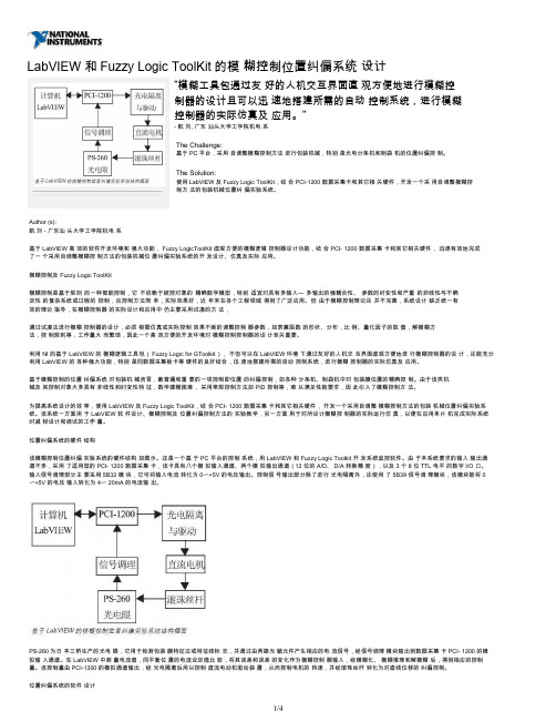
"- 航刘, 广东汕头大学工学院机电系The Challenge:基于PC平台,采用自调整模糊控制方法进行包装机械,特别是光电分条机和制袋机的位置纠偏控制。
The Solution:使用LabVIEW 及Fuzzy Logic ToolKit,结合PCI-1200 数据采集卡和其它相关硬件,开发一个采用自调整模糊控制方法的包装机械位置纠偏实验系统。
Author (s):航刘 - 广东汕头大学工学院机电系基于 LabVIEW 高效的软件开发环境和强大功能, Fuzzy LogicToolKit 直观方便的模糊逻辑控制器设计功能,结合PCI- 1200 数据采集卡和其它相关硬件,迅速有效地完成了一个采用自调整模糊控制方法的包装机械位置纠偏实验系统的开发设计、仿真及实际应用。
模糊控制及 Fuzzy Logic ToolKit模糊控制是基于规则的一种智能控制,它不依赖于被控对象的精确数学模型,特别适宜对具有多输入—多输出的强耦合性、参数的时变性和严重的非线性与不确定性的复杂系统或过程的控制,且控制方法简单,实际效果好,近年来在各个工程领域得到了广泛应用。
但由于模糊控制理论还并不完善,系统设计缺乏统一有效的理论指导,在模糊控制器的实际设计和应用中仍主要采用试凑的方法,通过试凑法进行模糊控制器的设计,必须根据仿真或实际控制效果不断的调整控制器参数,如隶属函数的形状、分布,比例、量化因子的取值,解模糊方法,控制规则等,工作量大而繁琐,因此一个高效方便的开发环境对模糊控制控制器的设计至关重要。
利用NI 的基于 LabVIEW 的模糊逻辑工具包( Fuzzy Logic for GToolkit),不但可以在 LabVIEW环境下通过友好的人机交互界面直观方便地进行模糊控制器的设计,还能充分利用 LabVIEW 的各种强大功能,特别是同数据采集板卡等硬件的良好结合,迅速地搭建所需的自动控制系统,进行模糊控制器的实际仿真及应用。
基于LabVIEW的模糊控制系统设计
基于LabVIEW的模糊控制系统设计
张永胜;高宏力;刘庆杰
【期刊名称】《仪表技术与传感器》
【年(卷),期】2012(000)003
【摘要】图形编程语言LabVIEW和模糊控制系统凭借其各自的特点在工业生产中得到广泛的应用,但是将两者结合的应用比较少.结合LabVIEW和模糊控制系统的优点,分析了LabVIEW中实现模糊控制系统的方法,利用PID and Fuzzy Logic Toolkit设计了一个基于LabVIEW的模糊控制器,并对频率为10.1 Hz,幅值为1的正弦波和三角波信号进行跟踪.结果表明:基于LabVIEW的模糊控制器结合了两者的优点,易于实现并具有良好的动态特性.
【总页数】3页(P27-29)
【作者】张永胜;高宏力;刘庆杰
【作者单位】西南交通大学机械工程学院,四川成都610031;西南交通大学机械工程学院,四川成都610031;西南交通大学机械工程学院,四川成都610031
【正文语种】中文
【中图分类】TP273.4
【相关文献】
1.基于LabVIEW的温室大棚温、湿度解耦模糊控制监测系统设计与实现 [J], 卢佩;刘效勇
2.基于LabVIEW起落架磁流变减震器模糊控制系统设计与分析 [J], 祝世兴;李健;
王博
3.基于LabVIEW的直流电机模糊控制系统设计 [J], 赵党军;杨帆;李国平
4.基于LabVIEW的直流电机模糊控制系统设计 [J], 赵党军;杨帆;李国平
5.基于LabVIEW的锂电池极片卷绕设备模糊控制系统设计 [J], 关朴芳
因版权原因,仅展示原文概要,查看原文内容请购买。
NI DAQ和LabVIEW构造模糊控制系统
NI DAQ和LabVIEW构造模糊控制系统关键词:模糊控制;LabVIEW;NI DAQ设备自动控制理论经过一个多世纪的发展,正由经典控制理论,现代控制理论向智能控制理论发展。
人工智能包括推理,学习和联想,是采用非数学式的方式,将人的思维模型化,并通过计算机来模仿。
目前计算机已充分体现了人类左脑的逻辑推理功能,正向右脑的模糊处理方向发展。
模糊控制作为近代控制理论中一种基于语言规则与模糊推理的高级控制策略和新颖技术,是智能控制的一个重要分支,近来发展迅速,应用广泛,效果显著,引人关注。
什么是模糊在我们日常生活中,经常有一些概念没有固定的标准,不能简单地用对或错,真或假来评判,而要用到一些不精确的词句来描述,比如,年轻、好、漂亮。
这些概念会因为判断对象变化而改变判断标准,所以是模糊的。
在人们的工作经验中,往往也存在了许多模糊的东西。
例如,炼钢时需要的钢水颜色、沸腾情况等模糊信息。
1965年美国加州大学L.A.Zadeh 教授最早提出了模糊这一概念,并用数学方式进行分析。
通常,对于一个论域E中讨论的集合A={a,b,c},对于论域中的任意元素x,可用特征函数表示是否属于A:(式1)式1用1和0来表示元素属于集合的真假,然而若是一个模糊的集合,比如说衣服是否漂亮,里面的元素a,b,c这3件衣服单纯用漂不漂亮表示显然不能更具体表征元素的性质。
模糊集合把特征函数的0和1这两个值,扩展到0到1之间的整个区间中,以隶属度μA(0≤μA≤1)来表示元素属于集合A的程度,比如衣服漂亮的程度。
这样,设三件衣服的漂亮程度分别为0.3,0.8和0.5,该模糊集合A可表示为A:{(a,0.3),(b,0.8),(c,0.5)}。
而隶属度函数可写成:(式2)可见模糊集合在多数情况下更能反应元素的特性,特征函数实际上就是隶属度函数的一个特例。
两个元素之间的某种联系,可以用关系R来表示,通常R用二元逻辑1和0表示元素之间是否存在此关系。
基于LabVIEW的直流伺服电机模糊PID控制系统
基于LabVlEW的直流伺服电机模糊PID控制系统LabVIEW-BasedFuzzyPIDControlSystemofDCServo-motor昊占涛-,z张桂香2(1湖南大学国家高效磨黼I程技术研究中心,长沙410082;2湖南大学机械与汽车工程学院,长沙410082)攘娶:论述了一种基予模糍PID算法的直流镯服电极控制系统,介缁了模糨PID算法及模糊控裁规鲻。
系统采用图形化的编程潜言LabVIEW,软件交互界面友好。
试验结果表明,采用该模糊PID控制器的系统能克服常规PID控制器的弊端,控制品质好,算法简单,具有实际应用价值。
关键词:直流伺服电视模糊控铡PIDLabVIEWAbstract:TheDCservo-motorcontrolsystembasedonfuzzyPIDalgorithmisintroduced。
ThefussyPIDalgorithmandtheregulationoffuzzycontrolarepresented.Thesystemhasafinesoftwareinterface,whichisrealizedbyLabVlEW。
TheresultsshowthatthefussyPIDcontrolsystemcanovercomethedrawbacksoftraditionalPIDcontroller,whichhasapracticalvalueofapplicationwithgoodcontrolperformanceandsimplealgorithm.Keywords:DCservo-motorfuzzycontrolPIDLabVIEW0引言直流伺服电视爨祷响应侠、低速平稳住好、潺速范围宽等特点,常用于实现精密谪速和位置控制的随动系统中,在工业、国防和民耀等领域内褥到广泛应瘸脚;所以,会理选择鸯漉饲服电机的控制方法。
X寸予充分发撂盔流箍鞭电梳的工作蔑麓鸯着积极的作用。
基于LabVIEW的模糊控制系统设计
个预先设计好 的后缀为 . f s的模糊控制系统文件到 系统 中。
p o u t n id vd al . B tt e a p ia in o h s w o i e s r lt ey l s . B ne r t g t e me to oh L b EW r d c i n ii u l o y u p l t ft e e t o c mb n d wa ea i l e s h c o v y i tg ai h r f t a VI n i b
K e o ds: b EW ;uzy c nto he r vru lisr m e t yw r La VI f z o r lt o y; it a n tu n
1 L b E 实 现 模 糊 控 制 的 方 法 a VI W 1 1 在 L b I W 中 实 现 模 糊 控 制 有 多种 方 法 : . a VE ( ) 用 Lb I W 中 的 CN 节 点 可 以 编 辑 或 者 调 用 已 经 1利 a VE I
Z A G Y n — e gG O H n — ,I ig i H N ogs n , A o g iLU Qn -e h l j ( co l f c a ia E g er g S uh et ioo gUnvri , h n d 1 0 1 C ia Sh o o h ncl n i ei ,o tw s Jatn ies y C e g u60 3 , hn ) me n n t
摘要: 图形 编 程 语 言 L b I W 和 模 糊 控 制 系统 凭 借 其 各 自的 特 点 在 工业 生产 中得 到 广 泛 的 应 用 , 是 将 两 者 结 合 的 a VE 但
应 用比较 少。结合 L b IW 和模 糊控制 系统的优点 , aVE 分析 了 L b IW 中 实现模 糊控制 系统 的方法 , aV E 利用 PD adF zy I n uz
基于LabVIEW的直流电机模糊控制系统设计
基于LabVIEW的直流电机模糊控制系统设计摘要:利用模糊控制算法实现了一个小型直流电机的转速控制系统。
用LabVIEW的模糊控制器设计工具进行模糊控制器的设计,通过NI-PCI6251完成实时速度采集以及电机转速控制。
实际运行表明该系统具有超调小,调节时间短以及振荡小的优点。
关键字:LabVIEW; 模糊控制; 转速控制; 数据采集卡Abstract: A control system of rotating speed of a small DC motor is implemented by using fuzzy control algorithm. The fuzzy controller is designed by the fuzzy controller design tool of LabVIEW. The control of rotate speed and real-time speed acquisition are accomplished by data acquisition card NI-PCI6251.The result demonstrates that the system has advantageous of small overshoot, setting time and oscillation.Keywords: LabVIEW; fuzzy control; rotating speed control; data acquisition card 模糊控制技术是以模糊集合论、模糊语言变量及模糊逻辑推理为基础的一种计算机数字控制,最早出现于上个世纪60年代,在其后的几十年中迅速发展。
目前模糊控制技术在控制领域的应用非常广泛。
LabVIEW则是一种面向仪器测量控制的图形化的编程语言,配合数据采集卡或其他外部设备可以非常方便的构成以计算机为核心的测量控制系统。
- 1、下载文档前请自行甄别文档内容的完整性,平台不提供额外的编辑、内容补充、找答案等附加服务。
- 2、"仅部分预览"的文档,不可在线预览部分如存在完整性等问题,可反馈申请退款(可完整预览的文档不适用该条件!)。
- 3、如文档侵犯您的权益,请联系客服反馈,我们会尽快为您处理(人工客服工作时间:9:00-18:30)。
LabVIEW的模糊控制系统设计(DOC 8页)基于LabVIEW的模糊控制系统设计摘要本文以LabVIEW为开发环境进行设计模糊控制器,将设计出的模糊控制器应用到温度控制系统中,实现了在有干扰作用的情况下对烤箱温度的控制,取得较好的控制效果。
关键词:虚拟仪器模糊控制热电偶AbstractThis paper is design issue is the use of LabVIEW fuzzy control, through the design of fuzzy control procedures to control the plant (oven) temperature. Finally, it comes ture control the temperature of oven even if there has disturb.Keywords:1引言虚拟仪器(LabVIEW),就是在以通用计算机为核心的硬件平台上,由用户设计定义虚拟面板,测控功能由软件实现的一种计算机仪器系统。
虚拟仪器的实质是利用计算机显示器的显示功能来模拟传统的控制面板,以多种形式表达输出结果,利用计算机强大的软件功能实现数据的运算、分析、处理和保存,利用I/O接口设备完成信号采集、测量与控制。
模糊控制的基本思想是利用计算机来实现人的控制经验,而这些经验多是用语言表达的具有相当模糊性的控制规则。
因为引入了人类的逻辑思维方式,使得模糊控制器具有一定的自适应控制能力,有很强的鲁棒性和稳定性,因而特别适用于没有精确数学模型的实际系统。
本文将模糊控制的基本思想应用到基于虚拟仪器的温度控制系统中。
通过热电偶测量烤箱实际温度,与给定值比较。
当测量温度与设定温度之间存在较大的偏差(e≥6℃)时,定时器产生占空比较大的脉冲序列,全力加热。
当系统温度与设定温度之间偏差小于6摄氏度,采用模糊控制算法。
模糊控制器根据误差和误差变化率,经过模糊推理输出脉冲序列的占空比的大小,经过固态继电器控制烤箱电源得通断,从而实现对烤箱温度的控制。
2系统组成图1 温度控制系统框图2.1 硬件组成传感器:热电偶;信号调理电路: SC-2345信号调理箱,SCC-TC02热电偶调理模块; 温度信号采集:DAQ 多功能数据采集卡PCI6014;执行器:DAQ 多功能数据采集卡上的定时/计数器,固态继电器; 对象:电烤箱。
2.2温度测量 1数据采集热电偶有三个较为突出的优点:其一,测量精度高。
因热电偶直接与被测对象接触,不受中间介质的影响;其二,测量范围广。
常用的热电偶从-50~+1600℃均可边续测量,某些特殊热电偶最低可测到-269℃(如金铁镍铬),最高可达+2800℃(如钨-铼);其三, 构造简单,使用方便。
热电偶通常是由两种不同的金属丝组成,而且不受大小和开头的限制,外有保护套管,用起来非常方便。
根据正、负极用材料的不同,热电偶分为B 、E 、J 、K 、R 、S 、T 、Y 型。
采用的是K 型热电偶,其正极为镍铬合金,负极为镍硅合金。
与其它类型的热电偶相比,K 型热电偶的线性较好,使用方便,因而在工业测量中被广泛使用。
而实际工作中,热电偶的自由端(冷端)是在室温下,为了得到正确烤箱温度,在查分度表时,要将室温对应的热电偶的热电势考虑进去,这就是冷端补偿。
2信号调理测温元件热电偶产生的是低电压信号,它需要进一步的放大、过滤以及线性化等处理. 本文采用SCC-TC02热电偶调理模块,通过SC-2345屏蔽盒与数据模糊控执电热—给输出采集卡相连。
SCC-TC02热电偶调理模块工作原理图如图2所示。
图2SCC-TC02热电偶调理模块工作原理图SCC-TC02接受三个信号:TC+ ,TC- ,和GND 。
TC+是热电偶的正极和TC-是热电偶负极。
接地端子连接到AIGND的E系列DAQ装置。
热电偶冷端信号和传感器信号测量的分别由E系列数据采集设备从X和X+8通道获得,其中X为0到7取决于操作者插TC02在SCC-2345的哪个插槽。
SCC-TC02热电偶调理模块的工作电路由两部分组成,一部分与热电偶连接,内部具有100倍的放大器和滤波器,将热电势放大,滤波;另一部分是用热敏电组测量室温的电路,用公式算出室温,对热电偶冷端补偿。
3数据处理利用Labview程序中多通道数据采集子VI将检测端数据和冷端数据两个通道的数据(第X通道和X+8通道)采集到数组中,再经过Index Array把数组分离开,然后分别处理。
3.1 热电偶检测到的数据处理第X通道采集上来的数据从数组输出并且取平均值(取平均值是为了消除随机误差),这个数值就是热电偶此时的电压值,把这个数乘1000(因为采集上来的电压信号的单位是伏特,而K型热电偶的分度表中的电压是毫伏),然后再除100,(因为热电偶调理模块里有一个100倍的放大电路)把结果输入到分段子程序中,进行分段子程序处理。
由于热电偶的温度与电压的关系是非线性的,为了把它分段线性化,所以就把温度分成若干段,认为在每段里,温度和电压的关系是线性的,可以用公式算出当时电压所对应的温度值。
分段的依据就是K 型热电偶的分度表,见表2.1T (℃) 0 10 20 30 40 50 6070 80 90 E (mV ) 0.000 0.397 0.7981.2031.6122.023 2.437 2.8523.2673.682T (℃) 100 110 120 130 140 150 160 170 180 190 E (mV ) 4.097 4.509 4.920 5.328 5.735 6.139 6.546.9417.340 7.739 T (℃) 200 210 220 230 240 250 E (mV )8.138 8.539 8.9409.343 9.747 10.153热电偶测温的部分,将检测到的温度以电压值的方式传到计算机,这就需要把电压值转换成温度,转换成温度才便于观测和显示。
以10℃为单位,根据分度表(参见下表1),分出12个等分的温度段,然后进行分段线性化,把采集到的电压分段,在每一段内,采用线性插值的方法计算,利用以下公式:经过分段子程序进行处理后,输出的数值是烤箱温度相对室温的差值。
热电偶信号处理子程序使用了一个case 结构,见图3:111212)(T V V V V TT T +-⨯--=图3 热电偶信号处理子程序3.2 利用热敏电阻测量室温进行冷端补偿第X+8通道采集上来的数据从数组输出并且取平均值,把这个数值输入到公式子程序中,经过公式子程序进行处理后,输出的数值就是室温。
热敏电阻的部分,利用冷端转换模块是根据SCC-TC02说明中所给出的公式: T (℃)=TK-273.15])c(lnR )b(lnR [a 13T T ++=K T7-4--3l0 .0l8703 l c 0 l 2.343l59 b 10l.29536l a ⨯=⨯=⨯=RT 是热敏电阻的欧姆值)5.2(5000TEMPOUTTEMPOUTT V V R -=通过公式编辑器,直接输入公式转换得出温度值。
由于采用的K 型热电偶的线性度较好,为了程序的简化,把热电偶的温度和室温的差值和室温直接相加,结果就是烤箱的温度。
4 模糊控制器设计模糊控制的实现要经过5个步骤:4.1确定模糊控制器的输入、输出语言变量系统误差e及其变化率e∆作为模糊控制器的输入变量,以u作为输出变量作为模糊控制器输出,模糊控制器是双输入单输出型。
4.2模糊化。
用模糊语言变量E、EC、U来描述偏差、偏差变化率及输出。
因为烤箱不能进行降温的操作,烤箱温度如果大于给定值,只能不加热自然降温,所以只考虑误差为正情况。
把6摄氏度分为7个档,即:{正很小,正小,正中小,正中,正中大,正大,正很大},记为E={PVS,PS,PMS, PM,PMB,PB,PVB}7档,E的论域为{0, +1, +2, +3,+4,+5,+6}。
同理:误差变化率e∆分成7档,即:{负大,负中,负小,零,正小,正中,正大}e 的模糊子集为:EC={NB, NM, NS, ZO, PS, PM, PB},量化EC的论域为{-3, -2, -1, 0, +1, +2, +3},输出变量U也分为7个档,即:{正很小,正小,正中小,正中,正中大,正大,正很大},记为U={PVS,PS,PMS, PM,PMB,PB,PVB}7档,U的论域为{0, +1, +2,=0.1。
误差隶属度、误+3,+4,+5,+6}。
量化因子分别为,则Ke=1,Kec=1,Ku差的变化率隶属度和控制量隶属度分别如表2、表3和表4所示表2 误差隶属度0 1 2 3 4 5 6E变量PVB 0.4 0.7 1 PB 0.4 0.7 1 0.7 PMB 0.4 0.7 1 0.7PM 0.4 0.7 1 0.7PMS 0.4 0.7 1 0.7PS 0.7 1 0.7PVS 1 0.7表3 误差的变化率隶属度∆E-3 -2 -1 0 1 2 3 变量PB 0.1 0.4 0.8 1.0 PM 0.2 0.7 1.0 0.2 PS 0.5 1.0 0.5ZR 0.5 1.0 0.5NS 0.7 0.8 1.0 0.5NM 0.8 1.0 0.7 0.5NB 1.0 0.8 0.4 0.1表4 控制变量隶属度0 1 2 3 4 5 6 U变量PVB 0.4 0.7 1 PB 0.4 0.7 1 0.7 PMB 0.4 0.7 1 0.7PM 0.4 0.7 1 0.7PMS 0.4 0.7 1 0.7PS 0.7 1 0.7PVS 1 0.74.3 形成模糊规则表系统的温度达到稳定,要经过振荡,超调,回调,反复调试,才能做到。
温度达到稳定的过度过程,可以分为四个阶段,如图4:图4 系统温度响应曲线t阶段:e>0 e∆<0 表示的物理意义是:系统温度未达到给定温度,0-1系统正在升温,相差大时,占空比应较大,相差小时,占空比减小甚至为0,考虑系统的滞后,应提前停止加热。
t-2t阶段:e<0 e∆<0 表示的物理意义是:系统温度超过到给定温1度,系统正在升温,超调,停止加热,占空比为0。
t-3t阶段:e<0 e∆>0 表示的物理意义是:系统温度超过到给定温2度,系统正在降温,超调,停止加热。
t-4t阶段:e>0 e∆>0 表示的物理意义是:系统温度未达到给定温3度,系统正在降温,应该加热,相差大时占空比大。
根据模糊变量e的赋值表、模糊变量e∆的赋值表、输出变量u的赋值表和对系统物理意义的分析,e∆为负值的时候,表示的物理意义是正处于升温的过程中;e∆为正值的时候,表示的物理意义是正处于降温的过程中;e∆为零的时候,表示的物理意义是的温度没有变化。