高分子分子量的主要测定方法
高分子物理实验报告稀溶液黏度法测定聚合物的分子量
⾼分⼦物理实验报告稀溶液黏度法测定聚合物的分⼦量实验⼀稀溶液黏度法测定聚合物的分⼦量⼀、实验⽬的1.了解聚合物分⼦量的统计平均的意义和黏度法表征,聚合物分⼦量的基本原理。
2.学会使⽤乌⽒黏度计。
3.掌握测定聚合物稀溶液黏度的实验技术。
⼆、实验原理采⽤稀溶液黏度法测定聚合物的分⼦量、所⽤仪器设备简单,操作便利,适⽤的分⼦量范围⼤,⼜有相当好的实验精确度,因此黏度法是⼀种⼴泛应⽤的测定聚合物分⼦量的⽅法。
但它是⼀种相对⽅法。
为特性黏数与分⼦量经验关系式中的常数要⽤其它测定分⼦量的绝对⽅法予以制定、并且在不同的分⼦量范围内,通常要⽤不同常数的经验式。
液体的流动是因受外⼒作⽤分⼦进⾏不可逆位移的过程、液体分⼦间存在着分⼦间作⽤⼒,因此当液体流动时,分⼦间就产⽣反抗其相对位移的摩擦⼒(内摩擦⼒)、液体的黏度就是液体分⼦间这种内摩擦⼒的表现。
黏度表⽰法相对黏度:表⽰溶液黏度相当于纯溶剂黏度的倍数。
η为⾼分⼦溶液的黏度ηo 为纯溶剂的黏度增⽐黏度:表⽰溶液黏度⽐纯溶剂黏度增加的分数。
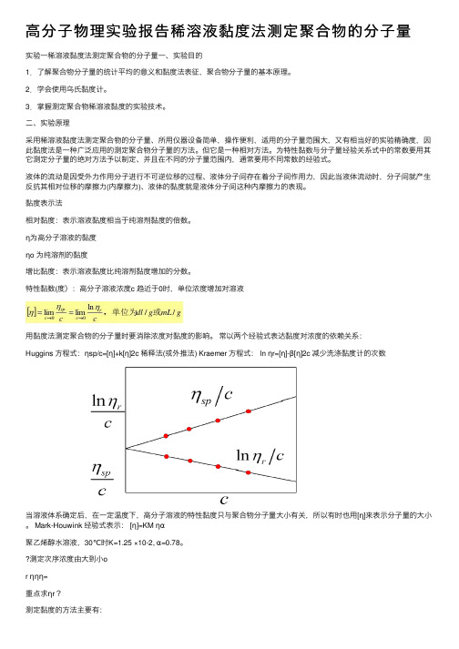
特性黏数(度):⾼分⼦溶液浓度c 趋近于0时,单位浓度增加对溶液⽤黏度法测定聚合物的分⼦量时要消除浓度对黏度的影响。
常以两个经验式表达黏度对浓度的依赖关系:Huggins ⽅程式:ηsp/c=[η]+k[η]2c 稀释法(或外推法) Kraemer ⽅程式: ln ηr=[η]-β[η]2c 减少洗涤黏度计的次数当溶液体系确定后,在⼀定温度下,⾼分⼦溶液的特性黏度只与聚合物分⼦量⼤⼩有关,所以有时也⽤[η]来表⽰分⼦量的⼤⼩。
Mark-Houwink 经验式表⽰: [η]=KM ηα聚⼄烯醇⽔溶液,30℃时K=1.25 ×10⁻², α=0.78。
测定次序浓度由⼤到⼩or ηηη=重点求ηr ?测定黏度的⽅法主要有:⑴⽑细管法(测定液体在⽑细管⾥的流出时间);⑵落球法(测定圆球在液体⾥下落速度);⑶旋筒法(测定液体与同⼼轴圆柱体相对转动的情况)测定⾼聚物溶液的黏度以⽑细管法最⽅便,本实验采⽤乌⽒黏度计测量⾼聚物稀溶液的黏度。
黏度法测定高分子化合物的分子量

二 实验原理
粘度系数η(kg.m-1.s-1):液体在流动中受的阻力。
二实验原理
同T下
0
增比粘度
相对粘度
sp
:(与溶剂比)溶液粘度增加的分数
r :溶液粘度与溶剂粘度的比值
高聚物溶液粘度
纯溶剂粘度 相对粘度
增比粘度
0 sp 1 r 1 0 0
hgr t
4
8Vl
η 为液体的粘度;ρ 为液体的密度; l为毛细管的长度;r为毛细管的半径; t为V体积液体的流出时间; V为流经毛细管的液体体积; h为流过毛细管液体的平均液柱高度; m为毛细管末端校正的参数。
1 1t1 2 2t 2
液t t r 0 水t0 t0
1. 将所测的实验数据及计算结果填入下表中: 原始溶液浓度C1 (g. mL-1);恒温温度 ℃ 溶剂流出时间t0_______、_________、________s t0平均= ________s
c c1=0.03 c2= t1/s t2/s t3/s t平均/s ηr lnηr ηsp ηsp/c lnηr/c
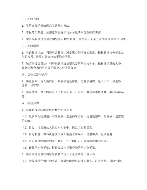
乌氏粘度计
恒温水浴槽
乌氏粘度计
四实验步骤
1. 调节恒温槽温度 37.0± 0.1 3.准备粘度计: B管和C管套橡皮管 垂直入恒温槽(螺旋夹固定) 水面浸没G球,检查垂直。
四 实验步骤
2. 溶液流经时间t的测定 移液管取右旋糖酐溶液4mL加入4ml水(记 C1=0.03g/ml),A口加入。 将B管夹紧,在C管打气(洗耳球),混合均 匀,恒温。 将C管夹紧,在B管将溶液抽至G球1/2处(洗 耳球); 松B管C管,使B管液体下落,当液面流到a刻 度,开始记时,降至b刻度,停止计时,测得a 、b刻度之间的液体流经毛细管所需时间t; 3次(相差0.2-0.3s),平均值。
分子量测定

分子量测定简介分子量(molecular weight)是指化合物中所有原子的相对质量总和。
分子量的测定是化学实验中常见的基本实验之一。
确定分子量可以帮助化学家了解化合物的结构和性质,从而更好地研究和应用化学物质。
在本文档中,我将介绍几种常用的方法来测定分子量。
1. 水蒸气密度法水蒸气密度法是一种常用且简便的测定分子量的方法。
该方法基于气体混合物在一定条件下的分子量比例关系。
通过测量气体混合物和纯净水蒸气的密度,可以计算出气体的分子量。
具体操作步骤如下:1.准备一个空气密度标准装置,该装置包括一个准确测量体积的玻璃管和一个可以控制温度和压力的装置。
2.将待测气体通过减压装置注入标准装置中,同时将水蒸气注入玻璃管。
待混合物达到平衡后,记录下温度和压力。
3.测量混合物的总体积,并记录下来。
4.根据实验参数计算气体的分子量。
2. 比色法比色法是通过测量溶液吸收特定波长的光的强度来确定溶液中物质的浓度,从而计算出分子量。
该方法适用于色谱法、光谱法、红外法等多种分析方法。
具体操作步骤如下:1.选取一款适用于目标溶液的比色计,调整仪器参数并进行校准。
2.将待测溶液转移到比色计中,使用已知浓度的溶液进行参比。
3.调整比色计的检测波长为目标物质的吸收峰波长。
4.测量目标溶液和参比溶液的吸光度,并计算出溶液的浓度。
5.根据溶液的浓度和溶质的摩尔浓度关系,计算出分子量。
3. 粘度法粘度法是一种利用溶液的粘度来测定溶质分子量的方法。
该方法适用于高分子化合物或具有高浓度的分子溶液。
具体操作步骤如下:1.准备一个稳定的粘度计和测量装置。
2.将待测溶液放入粘度计中,注意保持稳定和恒定的温度。
3.测量溶液的粘度,并记录下温度和压力。
4.对已知浓度的相似溶液进行对比测量,计算出待测溶液的相对粘度。
5.根据分子量与溶液相对粘度的关系,计算出分子量。
4. 凝胶渗透色谱法凝胶渗透色谱法(gel permeation chromatography, GPC)是一种常用于高分子化合物分子量测定的方法。
高分子量的测定实验报告
一、实验目的1. 了解高分子量的概念及其测定方法。
2. 掌握乌氏黏度计法测定聚合物平均分子量的原理及操作步骤。
3. 学会凝胶渗透色谱法测定聚合物平均分子量及其分子量分布的原理及操作步骤。
二、实验原理1. 乌氏黏度计法:利用乌氏黏度计测定聚合物溶液的黏度,根据黏度与分子量之间的关系,计算出聚合物的平均分子量。
2. 凝胶渗透色谱法:利用凝胶渗透色谱仪分离聚合物分子,根据分子量的大小,计算出聚合物的平均分子量及其分子量分布。
三、实验仪器与试剂1. 实验仪器:乌氏黏度计、凝胶渗透色谱仪、恒温水浴锅、电子天平、移液器、烧杯、试管等。
2. 实验试剂:聚合物溶液(已知分子量)、溶剂、凝胶渗透色谱柱、凝胶标准品等。
四、实验步骤1. 乌氏黏度计法测定聚合物平均分子量(1)配制聚合物溶液:准确称取一定量的聚合物,用溶剂溶解,配制成一定浓度的溶液。
(2)恒温:将溶液放入恒温水浴锅中,恒温至实验温度。
(3)测定黏度:将乌氏黏度计放入恒温水浴锅中,调整零点,记录温度。
(4)测定聚合物溶液的流出时间:打开阀门,记录溶液流出的时间。
(5)计算平均分子量:根据公式计算聚合物的平均分子量。
2. 凝胶渗透色谱法测定聚合物平均分子量及其分子量分布(1)凝胶渗透色谱柱的准备:将凝胶渗透色谱柱安装好,注入溶剂,排除气泡。
(2)样品的制备:准确称取一定量的聚合物,用溶剂溶解,配制成一定浓度的溶液。
(3)色谱分析:将样品注入凝胶渗透色谱仪,设定合适的流动相和流速,进行色谱分析。
(4)数据处理:根据色谱图,计算出聚合物的平均分子量及其分子量分布。
五、实验结果与分析1. 乌氏黏度计法测定聚合物平均分子量根据实验数据,计算得出聚合物的平均分子量为:Mw = 2.5×10^5 g/mol2. 凝胶渗透色谱法测定聚合物平均分子量及其分子量分布根据实验数据,聚合物的平均分子量为:Mw = 2.4×10^5 g/mol分子量分布:- 分子量小于1×10^5 g/mol的聚合物质量分数为10%- 分子量在1×10^5~5×10^5 g/mol的聚合物质量分数为70%- 分子量大于5×10^5 g/mol的聚合物质量分数为20%六、实验结论1. 通过乌氏黏度计法和凝胶渗透色谱法,成功测定了聚合物的平均分子量及其分子量分布。
气相渗透法测定高分子数均分子量详解

Vapor Pressure OsmometerIntroductionDetermination of the molar mass of polymers is of considerable importance because the chain length is a controlling factor in the evolution of solubility, elasticity, fiber formation, and mechanical strength properties. Methods used to determine the molar mass are either relative or absolute. Relative methods require calibration with samples of known molecular weight and absolute methods require no such calibration. This report will focus on the use of membrane and vapor pressure osmometry to determine the number average molecular weight (Mn). These techniques are useful in different Mn ranges and depend on the change in osmotic pressure and the lowering of vapor pressure (respectively) by polymers in solution.Membrane OsmometryIntroduction and TheoryMembrane osmometry is an absolute technique which determines Mn. The solvent is separated from the polymer solution by a semipermeable membrane which is tightly held between the two chambers. One chamber is sealed by a valve with a transducer attached to a thin stainless steel diaphragm which permits the measurement of pressure in the chamber continuously. The solvent chamber is filled with solvent and closed to the atmosphere except for the solvent passage through the membrane while the solute chamber is left open to the atmosphere. The solute cannot flow in this case but the solvent can flow through the membrane. The chemical potential of the solvent is much higher than that of the solute, therefore there is a tendency for flow to occur from the solvent through the membrane to the polymer solution. Because the solvent is permitted through the membrane a change in concentration causes the solvent to diffuse to the solute side of the chamber. As this occurs, the pressure of the solvent decreases until the pressure difference across the membrane just counteracts the chemicalpotential difference caused by the solute. This pressure reduction required to equilibrate the chemical potential on both sides of the membrane is regarded as the osmotic pressure. It is the pressure required in order to affect the activity of the solvent and solution equal to that of the solution. The osmotic pressure is related to the change in chemical potential by the following equation:(µ1−µ10)=-V1πwhere µ10= chemical potential of pure solventµ1 = chemical potential of solvent in solutionV1 = molar volume of solvent in solutionπ = osmotic pressureExamining the osmotic pressure in terms of the free energy of mixing phenomena, the change in chemical potential can be related to the polymer molecular weight by substitution of the above equation into the following:(µ1−µ10)=-RT[c2V1/M2+ν22(1/2−χ1)c22] where Μ2= polymer molecular weightν2 = partial specific volume of polymerχ = interaction parameterc2 = solute concentrationThe relationship of molecular weight to osmotic pressure is then simplified to:π/c2=RT/M2+RTν22/V1(1/2-χ1)c2The first term of this equation is the van’t Hoff expression for osmotic pressure at infinite dilution. The second term is the deviation from ideal behavior of the polymer solution and is related to the second virial coefficient. The relationship between the second virial coefficient and the interaction parameter is illustrated by:A=RTν22/V1(1/2-χ1)When the interaction parameter is equal to 1/2 and the second virial coefficient is zero, then the osmotic pressure is governed by the ideal solution law.Experimentally, in calculating the molecular weight, osmotic pressure must be measured at several different concentrations. π/C2 is determined for each concentration and plotted π/c2 versus c2, extrapolating the concentration to zero. The slope of the resultant line is the second virial coefficient and the molecular weight is calculated by the intercept.Procedure for Use of Membrane OsmometerThe instrument on the polymer floor contains two main components, the cell assembly and the electronics-recorder assembly. Membrane conditioning is extremely important in using this technique. Membranes are usually cellulose derivatives and shipped in alcohol or aqueous solution. For aqueous solutions, simply rinse the membrane off with distilled water and place in the osmometer. The distilled water needs to be rinsed through the instrument several times while stabilizing the cell temperature. When an organic solvent needs to be used in place of water, several steps need to be taken in order to gradually introduce the membrane to this solvent. Every two hours, the concentration of a solution containing water and isopropanol is increased until a 100% concentration of isopropanol is used. Then isopropanol and the chosen organic solvent are used in the same manner described above until a 100% concentration of the organic solvent is used. Conditioning membranes in organic solvents causes the membranes to shrink therefore the membrane must have a larger diameter initially in order to compensate for this shrinkage. The required diameter for our instrument is 50mm.The next step is to set the temperature controls to coarse 2 and fine 200 and turn on the instrument’s power. Turn the pressure range gauge to 10 and set the recorder range to 1mV. The membrane is installed by first removing the top half of the cell cover and adding solvent to the cell assembly via syringe. Place the membrane (the membrane always needs to be wet with solvent so the membrane will not dry out) between the two aluminum plates and trim the membrane to the correct size to fit the center of the circular ring. Cover the membrane with solvent and tighten the membrane onto the circular ring. Fill the glass level tube with solvent and open all valves, pushing the solvent through three times. Close the solution drain valve and flush with solvent three times and then close the solvent drain valve and flush the solvent chamber three times. Close the solution drain valve and lower the level in the inlet tube with the solution drain valve to the top of the Swagelok fitting. Replace the cell cover and allow the instrument’s cell temperature to stabilize. It is very important to remove air from both sides of the membrane in order to obtain accurate results. Open the solution drain valve in order to reduce the level to a reference level of sixty percent. Close the solvent inlet valve slowly and reduce that level to sixty percent.The instrument is now ready to be calibrated. Connect the glass calibration tube to the inlet tube and then fill with solvent. Reduce the level in the calibration tube to the top mark and adjust the recorder to zero. Then reduce the solvent level 5 cm to the second mark on the tube. Adjust the calibrate control on the front of the panel to provide a half-scale reading. Then further reduce the solvent 10 cm from the top mark and calibrate as stated above. Remove the calibration tube and reset to the sixty percent reference point. It is important to note that if water is not the solvent used, then the specific gravity of the solvent needs to be multiplied by the chart recorder reading during calibration in order to obtain accurate results.It is a good idea to run a test sample before making measurements on the polymer sample. To obtain the molecular weight of the polymer sample, the general requirement is to take measurements at three to four different concentrations. These solution concentrations should be in the range of 10g per liter to 1.8g per liter. Close the solvent inlet valve and set the solvent level to a reading of 60 and allow the cell and the recorder to stabilize. Then add 0.5 to 1.0 ml of the polymer solution and open the solution drain valve until that level meter also reads 60. Do not allow the sample level to fall below the reference level. Allow for stabilization and read the osmotic pressure off of the recorder in cm of solvent pressure. Do this for each solution in order of increasing concentration and record all osmotic pressure results. Divide each pressure by the corresponding concentration and plot these values versus concentration. The intercept is then used to calculate the molecular weight.Advantages and DisadvantagesThe problems of this technique are caused mainly by the membrane. There are problems with membrane leakage and asymmetry. Membrane asymmetry is observed when both cells are filled with the same solvent but have a pressure difference between the two cells caused by membrane leakage, compression, solute contamination, or temperature gradients. Ballooning is another problem which is caused by pressure differentials and is detected by measuring the pressure change as the solvent is added or removed from the solvent cell. This effect is due to the viscoelastic nature of the membrane used. Rapid membrane degradation can also be a problem if harsh solvents are used or if the membrane is not keep moistened. Carefulpreparation of the membrane is also needed in order to ensure no holes are present. The presence of dissolved air is also a problem, so all solvents and solutions must be degassed before insertion into the cells. Overestimation of molecular weight can occur if low molecular weight molecules penetrate the membrane. This causes a decrease in π by not being on the sample side and compensates by changing the chemical potential on the solvent side. Therefore, polymers of high polydispersity are not well suited for membrane osmometry. Polyelectrolytes can cause a problem due to the fact that π/C values may be higher for these solutions in the absence of added salt and may increase with dilution.The main advantage of membrane osmometry is that it yields an absolute Mn for a polymer and calibration with standards is not required. Low molecular weights can be tolerated because they readily equilibrate on both sides of the membrane. Results are easily obtained for graft or copolymers because membrane osmometry is independent of chemical heterogeneity. This method is applicable to polymers having a broad range of molecular weights with the low end being governed by membrane permeability and the upper limit determined by the smallest osmotic pressure that can be measured. The most common range for determining molecular weights by this method is 5,000 to 500,000 (5000 for the state of the art instruments). The most common membranes typically can determine Mn as low as 10000-20000. Membrane osmometry also provides information about polymer-solvent interactions derived from the second virial coefficient.Vapor Pressure OsmometryIntroductionThe determination of Mn by the use of vapor pressure osmometry operates on the principle that the vapor pressure of a solution is lower than that of the pure solvent at the same temperature and pressure. At sufficiently low concentrations, the magnitude of the vapor pressure decrease is directly proportional to the molar concentration of solute. Monitoring vapor pressure versus a change in concentration of solute can be used in a manner similar to that of membrane osmometry.The derivation to relate Mn to vapor pressure is founded in the basic equations of dilute solution chemistry and physical chemistry. In a dilute solution, the vapor pressure of a solvent is given by Raoult’s Law:P1 = P10 x1where P1 = partial pressure of solvent in solutionP10 = vapor pressure of pure solventx1 = mole fraction of solventBy definition, x1 = 1-x2 where x2 is the mole fraction of solute so P1 = P10 (1-x2)and P10 - P1 = P10x2. The vapor pressure lowering is defined as ∆P = P10 - P1 and will also equal P10x2. For very small temperature changes that are associated with vapor pressure osmometry, it is assumed that T, ∆H v, and p are constant. Now, the Clausius-Clapeyron equation [dp/dT = (p∆H v)/(RT2)] can be integrated to yield:∆T = [(RT2)/( p∆H v)] - ∆P where p = vapor pressureT = absolute temperature∆H v = enthalpy of vaporizationR = gas constantSubstitution of the equations yields ∆T = (RT2P10x2)/(p∆H v) and for small pressure changes, P10 = p, so that ∆T = (RT2x2)/(∆H v). By definition:x2 = n2/(n1 + n2) where n1 = number of moles of solventn2 = number of moles of soluteFor very small n2 the relation will reduce to n2/n1 and plugging back into the temperature equation gives:∆T = (RT2/∆H v) * (C2/m2) * (m1/1000) where C2 = solute concentration (g/kg)simplified ∆T = K1(C2/m2) m2 = solute molecular weightm1 = solvent molecular weightA voltage change is measured in most vapor pressure osmometry instruments and is proportional to the temperature difference and is needed for all calculations:∆V = (K C2 )/ m2K is the calibration factor for the instrument and is determined by measuring ∆V and C2 for a series of known molecular weight (m2) species. K can then be used in the reverse fashion to determine the Mn of unknowns.Instrumentation for Vapor Pressure OsmometryVapor pressure is not measured directly due to difficulties in sensitivity, but is measured indirectly by using thermistors to measure voltage changes caused by changes in termperature. The polymer floor model is a Model 233 Molecular Weight Apparatus by Wescan Instruments, Inc. In this model, two thermistors are placed in the measuring chamber with their glass enclosed sensitive bead elements pointed up. The thermistors are covered with pieces of fine platinum screen to ensure a constant volume of the analyte is present on the bead for each measurement. (Another common model has the thermistors pointing upward, but has a drawback of delivering a constant amount of liquid to the surface each time.) The chamber contains a reservoir of solvent and two wicks to provide a saturated solvent atmosphere around the thermistors. If pure solvent on one thermistor is replaced by solution, condensation of solvent into the solution from the saturated solvent atmosphere will proceed. Solvent condensation releases heat, so the thermistor will be warmed. Condensation will continue until the thermistor temperature rises enough to bring the solvent vapor pressure of the solution up to that of pure solvent at the surrounding chamber temperature.The Model 233 has two cylindrical baffles placed inside an aluminum chamber around the two upward pointing thermistors. Each baffle consists of a metal cylinder and a porous paper wick. The wick provides a large surface area for the solvent and its transfer to the atmosphere inside the chamber to ensure saturation with solvent vapor. The detector for the 233 consists of a Wheatstone bridge, two thermistors, an oscillator for bridge power, AC amplifier, a synchronousselector, filter, and digital panel meter. Two silicone molded heaters are placed around the cylinder so that they cover about 80% of its surface. A precision controller can control the temperature to a few thousandths of a degree. Coarse and fine controls are calibrated to given temperatures and are set on the control panel.Operational ProceduresThe first step in preparing for a VPO run is to clean the chamber assembly. The chamber is removed form the oven, revealing the baffles, wicks, and thermistors. Gloves should be worn to prevent oils from the hands transferring to the chamber. The platinum gauze coverings of the thermistors are carefully removed with tweezers and placed in a solution of the solvent for which the new samples will be run. The uncovered thermistors and chamber are fully rinsed with the solvent and new wicks placed in the assembly. The chamber is reassembled with the gauze in place and 20 mL of solvent poured into the center cylinder over the thermistors. The injection syringes are then removed, cleaned with solvent, loaded with appropriate solutions or solvents, and returned to the apparatus. The Model 233 is capable of heating the syringes separately from the chamber, but this is seldom used for floor measurements. The temperature control should be set to the appropriate number and the instrument allowed to reach operating temperature. This is usually started before cleaning and allowed to warm and equilibrate for at least one hour.Calibration with materials of known molecular weight must precede measurement for unknowns to determine the K value. Requirements for standards are vapor pressure no more than 0.1% of that of the solvent, high purity, solubility, and formation of ideal solutions (optional). Sucrose octaacetate is the standard of choice for organic solvents and simple sucrose or mannitol are excellent for aqueous calibration. Sample running is the same for standards and unknowns. Operating temperature for the solvent of choice is determined from a chart in supplied application notes.Five solutions of the sample are prepared ranging in concentration from 0.7 g/L to 20 g/L based on the expected MW of the sample. The ZERO control on the operating panel is adjusted to get a reading on the meter between 0 and 10. With pure solvent in both syringes, add about0.03 ml of solvent to both thermistors. This task is simplified by marked screw drives that inject the needles. 0.03 mL will equal 2 full turns of the screws. After each addition, the screws are turned back 1 turn to prevent small drops from falling on the thermistors. Generally, the reading will go off scale and then return to a level value. Adjust the ZERO control to get a reading between 0 and 10 and repeat. Calculate the average value of the trials. The sample syringe is then filled with the most dilute polymer solution and turned until the meter goes off scale, then 30 seconds later, 3 turns. Remember to turn back the screw after each addition. This cleans the thermistor of the previous solution/solvent run. Now, the first real measurement takes place with 2 turns for both the solvent syringe and sample syringe. The voltage is read after stabilization. Three or more trials for the same sample are run and an average calculated. Repeat for each concentration and record. Finally, subtract the pure solvent voltage from these readings to give the true ∆V for the various concentrations.The data is plotted as ∆V/C versus C (g/L) and a best fit straight line is extrapolated to zero concentration. Adjusting our voltage equation for the plot at zero concentration, the following relations are derived:Κ = ∆V/C * m2When using known m2 to determing Km2 = (K) / (∆V/C)After calibration with unknown m2 sampleMW Ranges for VPOIf experimental factors are controlled very carefully, very accurate M n numbers can be achieved. MW’s below 1000 are determinable with a precision of 0.5 %. The lower limit of MW is technically only limited by the vapor pressure of the sample, but useful lower limits are in the 250 level. Upper MW limits as high as 400000 have been reported, but the instrumental sensitivity determines this factor. Most commercial instruments can reach 100000, but it is safest to assume the upper limit as 50000. It should be further noted that the temperature change is inversely proportional to the solvent heat of vaporization. Therefore, benzene and chloroform will have the best sensitivity and water would have the worst. The upper limit for molecular weights in water will be 20000-25000 and this with only the most sensitive instrument.VPO and Membrane Osmometry as Complimentary MethodsThe most obvious comparison of the methods shows that VPO is useful in a lower MW range than membrane osmometry. Membrane osmometry does not require calibration with a molecular weight standard as does vapor pressure osmometry. Determination of property to be measured is the driving force between choice of the two methods. For example, a polymer that is used for injection molding is to be analyzed. The behavior in the molding instrument will depend on the amount of low molecular weight polymer in the material. VPO is the best choice, since membrane osmometry would exclude the low MW portion. On the other hand, a polymer with no low molecular weight polymer present but with additives such as antioxidants or plasticizers would give erroneous M n values if VPO was used due to inclusion in the measurement of the additives’ MW. Membrane osmometry would be preferred. In an interesting case, polyelectrolytes must be analyzed with a significant amount of electrolyte present to account for their charged behavior. VPO will respond primarily to the salt added and completely eliminate the polymer signal. Membrane osmometry will allow the salt to equilibrate through the membrane and the final osmotic pressure will be due to only the polymer. Using both methods to analyze a possibly highly dispersed polymer will allow a better understanding of the low and high MW ends of the distribution curve.Recent Applications for Combining Osmometry With Other TechniquesIn a recent issue of Macromolecules , Lehmann and Kohler reported the use of membrane osmometry as an online detector in correlation with size exclusion chromatography. This allows for absolute molar mass detection. The use of a membrane osmometer as an absolute online detector is important because especially for polar polymers, adsorptive interaction between the column and the polymer in SEC cannot be disregarded. This can cause erroneous results when using the universal calibration technique to determine molecular weight. Colligative properties like osmotic presssure are only sensitive to the number of molecules in solution. Therefore, an absolute SEC calibration can be obtained by a simultaneous measurement of concentration and of a colligative property. In this case membrane osmometry was employed due to its sensitivity.When the experiments were performed using this technique, the RI detector of the SEC setup was replaced with a membrane osmometer.The authors redesigned the osmometer because a cell with a flat membrane is not suited for a continuous flow operation. They designed an osmometer containing cylindrical symmetry which contains a semipermeable membrane and an outer glass tube. The polymer solution then flows through the bore of the membrane capillary. The reference cell is filled with solvent and is the volume between the membrane and the outer glass tube. The solution chamber inside the capillary can be easily flushed, ideally suiting it for use as a flow cell and the balloon effect is negligible. The semipermeable support membrane is a highly asymmetric poly(acrylonitrile) hollow fiber which contains an inner separating layer. The inner side or solution side of the support membrane is coated with a dilute solution of poly(dimethylsiloxane). This composite membrane is perfectly suited for online detection because of its mechanical stiffness, high solvent permeability, and low molar mass cutoff. The membrane osmometer and membrane combined, meet the requirements for online detection: low cell volume, short response time, and low molar mass cutoff.The instrument was tested on both batch and continuous flow operations withpoly(styrene) standards. The results were in agreement with the suggested molar masses. Response time is very short in comparison to a standard membrane osmometer and this leads to slight peak broadening. The problems that the authors find need more work are reduction of this peak broadening and a reduction of the pressure noise level along with the elimination of long term baseline drifts. However, this technique has been shown to successfully measure absolute molecular weights by the combination of size exclusion chromatography with online detection using membrane osmometry.References1. Barth and Mays, Modern Methods of Polymer Characterization . New York: Wiley and Sons, 1991, pp. 208-222.2. Burge, D. American Laboratory. June Issue (1977).3. Cowie, J. Polymers: Chemistry and Physics of Modern Materials. New York: Chapman andHall, 1991, pp. 164-166.4. Lehmann, U. and W. Kohler, Macromolecules. 1996, 29, 3212.5. Morris, C. and H. Coll Determination of Molecular Weight. New York: Wiley and Sons,1989, pp. 15-44.6. Rabek, J. Experimental Methods in Polymer Chemistry. New York: Wiley and Sons, 1980,pp. 78-85, 95-97.7. Recording Membrane Osmometer Instruction Manual. Model 231.。
分子量实验报告
一、实验目的本次实验旨在通过测定不同样品的分子量,了解分子量与样品性质之间的关系,并掌握常用的分子量测定方法。
二、实验原理分子量是高分子化合物的重要性质之一,它反映了高分子链的长短。
分子量的测定方法主要有重量法、粘度法、渗透压法、光散射法等。
本实验采用重量法、粘度法和渗透压法测定样品的分子量。
三、实验材料与仪器1. 实验材料:聚乙烯醇(PVA)、聚丙烯酸(PAA)、聚乙烯(PE)等高分子化合物。
2. 实验仪器:分析天平、乌氏黏度计、渗透压计、恒温箱、移液器等。
四、实验步骤1. 重量法测定分子量(1)称取一定量的PVA、PAA、PE样品,分别放入三个锥形瓶中。
(2)将锥形瓶放入恒温箱中,在规定温度下溶解样品。
(3)用移液器将溶解后的样品溶液转移至已知分子量的标准溶液中,使样品溶液的浓度与标准溶液的浓度相等。
(4)将混合溶液放入分析天平中,称量其质量。
(5)根据样品溶液的质量、浓度、标准溶液的分子量及体积,计算样品的分子量。
2. 粘度法测定分子量(1)将乌氏黏度计清洗干净,并用蒸馏水冲洗。
(2)在规定温度下,将样品溶液倒入黏度计的两个垂直管中。
(3)启动计时器,记录样品溶液通过黏度计的时间。
(4)根据样品溶液的浓度、温度、黏度计的几何参数,计算样品的分子量。
3. 渗透压法测定分子量(1)将渗透压计清洗干净,并用蒸馏水冲洗。
(2)将样品溶液倒入渗透压计的两个容器中,使样品溶液的浓度与已知分子量的标准溶液的浓度相等。
(3)记录渗透压计的示数。
(4)根据样品溶液的浓度、渗透压计的示数、标准溶液的分子量,计算样品的分子量。
五、实验结果与分析1. 重量法测定分子量结果:样品名称 | 分子量(g/mol)------- | --------PVA | 7.5×10^4PAA | 1.2×10^5PE | 5.0×10^52. 粘度法测定分子量结果:样品名称 | 分子量(g/mol)------- | --------PVA | 7.8×10^4PAA | 1.3×10^5PE | 5.2×10^53. 渗透压法测定分子量结果:样品名称 | 分子量(g/mol)------- | --------PVA | 7.6×10^4PAA | 1.4×10^5PE | 5.1×10^5通过对比三种方法的测定结果,可以发现,重量法、粘度法和渗透压法测定得到的分子量相近,说明这三种方法都可以用于分子量的测定。
高分子分子量测定方法的研究
高分子分子量测定方法的研究高分子材料在生活中的应用越来越广泛,例如塑料、橡胶、纤维等。
因此,高分子材料的质量控制和研究变得越来越重要。
高分子材料的分子量是其物理、化学和力学性质的重要指标,因此分子量的精确测定是高分子材料研究的一个重要方面。
目前,已经开发了多种高分子分子量测定方法,包括粘度法、光散射法、凝胶渗透色谱法、质谱法等。
本文将介绍一些高分子分子量测定方法的原理、特点和应用。
一、粘度法粘度法是高分子分子量测定的最早的方法之一,其原理是:高分子在溶液中运动时,会与溶剂分子相互摩擦和撞击,产生阻力,导致溶液的整体粘度增加。
粘度与分子量成反比,因此可以用粘度法来测定高分子的分子量。
具体地,用天平称取不同浓度的高分子溶液,在特定的温度下,测量溶液的粘度。
将粘度数据与相应的浓度计算出粘度平均分子量,从而得到分子量的概略值。
粘度法的优点是操作简单、不需要复杂的仪器设备、测量时间短、成本低廉。
但是,粘度法在分子量高于10万时,其精度受到很大限制。
此外,不同高分子之间粘度测量结果的可比性较差,因此需要对不同高分子进行标准化处理。
二、光散射法光散射法是一种测量高分子分子量的准确方法,可以用来测量高分子的绝对分子量、分子量分布和形态结构等。
光散射测量的原理是: 测量高分子溶液中光线的散射强度,改变光线方向或波长,可以获得不同范围分子量的散射强度分布,从而测量高分子的分子量特性。
与粘度法相比,光散射法更适合于测量高分子的分子量分布宽泛和形态结构不规则的情况。
三、凝胶渗透色谱法凝胶渗透色谱(GPC)法是一种广泛应用的高分子分子量测定方法。
其原理是: 利用凝胶为分子分离提供渗透分子的溶剂黏度,嵌入凝胶内进行分子量分布测定。
凝胶作为一种多孔元素或分子网络,具有分子筛、分子导向、渗透、化学识别等作用。
当高分子涂布在凝胶表面时,由于凝胶中的分子间间隙比高分子分子大,高分子的长链会被凝胶筛选,而短链则可以穿过凝胶,在洗涤溶液中被洗出,使溶液分子量分布向小分子倾斜。
高分子分子量的主要测定方法
高分子分子量的主要测定方法凝胶渗透色谱法(GPC)是目前最常用的测定高分子分子量的方法之一、该方法通过溶液在固定温度下通过分子量递增的多孔型固定相上进行分离,然后测定溶液通过时间和多孔固定相间时间之比,从而计算出分子量。
该方法适用于多种高聚物,不受化学结构和溶剂的影响,具有精密度高、准确度好的特点。
流变法是通过测定高聚物在应力或应变下的变形特性来间接测定分子量。
根据流变曲线的形状和参数,可以计算出高聚物的分子量。
常用的流变方法有旋转流变法、振动流变法和剪切流变法等。
流变法可以对高聚物的流变性质进行全面的研究,但在测定分子量时,需要进行一定程度的假设和简化。
光散射法是通过测量光散射的强度和角度来计算高聚物的分子量。
高分子分子量越大,其颗粒的大小也越大,因此散射光的强度也越大。
通过测量散射光的强度和角度,可以得到高聚物的分子量分布。
光散射法不需要特殊的样品处理,适用于固态和溶液态样品,但需要较昂贵的设备和较复杂的分析计算方法。
核磁共振法(NMR)是通过测量高聚物中的特殊核的共振峰来计算分子量。
NMR可以提供高分辨率的谱图和详细的结构信息,对于一些特殊结构的高聚物尤为适用。
但由于测定时间长、灵敏度低等限制,目前核磁共振法在测定高分子分子量方面的应用较少。
除了这些主要的测定方法外,还有一些其他的方法可以用来测定高分子分子量,比如粘度法、沉降法、电泳法等。
这些方法各有特点,选择合适的测定方法取决于样品的性质、测量的目的和仪器设备的可用性等因素。
总之,高分子分子量的测定方法各有特点和适用范围,需要结合具体情况选择合适的方法进行测定。
随着科学技术的发展和仪器设备的改进,高分子分子量测定方法也将越来越精确和方便。
- 1、下载文档前请自行甄别文档内容的完整性,平台不提供额外的编辑、内容补充、找答案等附加服务。
- 2、"仅部分预览"的文档,不可在线预览部分如存在完整性等问题,可反馈申请退款(可完整预览的文档不适用该条件!)。
- 3、如文档侵犯您的权益,请联系客服反馈,我们会尽快为您处理(人工客服工作时间:9:00-18:30)。
高分子分子量的主要测定方法
用途
高聚物的分子量及分子量分布,是研究聚合物及高分子材料性能的最基本数据之一。
它涉及到高分子材料及其制品的力学性能,高聚物的流变性质,聚合物加工性能和加工条件的选择。
也是在高分子化学、高分子物理领域对具体聚合反应,具体聚合物的结构研究所需的基本数据之一。
表征方法及原理
1.粘度法测相对分子量(粘均分子量Mη)
用乌式粘度计,测高分子稀释溶液的特性粘数[η],根据Mark-Houwink公式[η]=kMα,从文献或有关手册查出k、α值,计算出高分子的分子量。
其中,k、α值因所用溶剂的不同及实验温度的不同而具有不同数值。
2.小角激光光散射法测重均分子量(Mw)
当入射光电磁波通过介质时,使介质中的小粒子(如高分子)中的电子产生强迫振动,从而产生二次波源向各方向发射与振荡电场(入射光电磁波)同样频率的散射光波。
这种散射波的强弱和小粒子(高分子)中的偶极子数量相关,即和该高分子的质量或摩尔质量有关。
根据上述原理,使用激光光散射仪对高分子稀溶液测定和入射光呈小角度(2℃-7℃)时的散射光强度,从而计算出稀溶液中高分子的绝对重均分子量(MW)值。
采用动态光散射的测定可以测定粒子(高分子)的流体力学半径的分布,进而计算得到高分子分子量的分布曲线。
3.体积排除色谱法(SES)(也称凝胶渗透色谱法(GPC))
当高分子溶液通过填充有特种多孔性填料的柱子时,溶液中高分子因其分子量的不同,而呈现不同大小的流体力学体积。
柱子的填充料表面和内部存在着各种大小不同的孔洞和通道,当被检测的高分子溶液随着淋洗液引入柱子后,高分子溶质即向填料内部孔洞渗透,渗透的程度和高分子体积的大小有关。
大于填料孔洞直径的高分子只能穿行于填料的颗粒之间,因此将首先被淋洗液带出柱子,而其他分子体积小于填料孔洞的高分子,则可以在填料孔洞内滞留,分子体积越小,则在填料内可滞留的孔洞越多,因此被淋洗出来的时间越长。
按此原理,用相关凝胶渗透色谱仪,可以得到聚合物中分子量分布曲线。
配合不同组分高分子的质谱分析,可得到不同组分高分子的绝对分子量。
用已知分子量的高分子对上述分子量分布曲线进行分子量标定,可得到各组分的相对分子量。
由于不同高分子在溶剂中的溶解温度不同,有时需在较高温度下才能制成高分子溶液,这时GPC柱子需在较高温度下工作。
4.质谱法
质谱法是精确测定物质分子量的一种方法,质谱测定的分子量给出的是分子质量m对电荷数Z之比,即质荷比(m/Z)过去的质谱难于测定高分子的分子量,但近20余年由于我的离子化技术的发展,使得质谱可用于测定分子量高达百万的高分子化合物。
这些新的离子化
技术包括场解吸技术(FD),快离子或原子轰击技术(FIB或FAB),基质辅助激光解吸技术(MALDI-TOF MS)和电喷雾离子化技术(ESI-MS)。
由激光解吸电离技术和离子化飞行时间质谱相结合而构成的仪器称为“基质辅助激光解吸-离子化飞行时间质谱” (MALDI-TOF MS 激光质谱)可测量分子量分布比较窄的高分子的重均分子量(Mw)。
由电喷雾电离技术和离子阱质谱相结合而构成的仪器称为“电喷雾离子阱质谱”(ESI- ITMS 电喷雾质谱)。
可测量高分子的重均分子量(Mw)。
5.其他方法
测定高分子分子量的其他方法还有:端基测定法,沸点升高法,冰点降低法,膜渗透压法,蒸汽压渗透法,小角X-光散射法,小角中子散射法,超速离心沉降法等。