曼昆宏观经济经济学第九版英文原版答案3
曼昆《宏观经济学》第9版章节习题精编详解(失业)【圣才出品】

曼昆《宏观经济学》(第9版)章节习题精编详解第2篇古典理论:长期中的经济第7章失业一、概念题1.自然失业率(natural rate of unemployment)答:自然失业率又称“有保证的失业率”、“正常失业率”、“充分就业失业率”等,它是经济围绕其波动的平均失业率,是经济在长期中趋近的失业率,是充分就业时仍然保持的失业水平。
自然失业率是在没有货币因素干扰的情况下,让劳动市场和商品市场自发供求力量起作用时,总供给和总需求处于均衡状态时的失业率。
“没有货币因素干扰”是指失业率的高低与通货膨胀率的高低之间不存在替代关系。
自然失业率决定于经济中的结构性和摩擦性的因素,取决于劳动市场的组织状况、人口组成、失业者寻找工作的能力愿望、现有工作的类型、经济结构的变动、新加入劳动者队伍的人数等众多因素。
任何把失业降低到自然失业率以下的企图都将造成加速的通货膨胀。
任何时候都存在着与实际工资率结构相适应的自然失业率。
自然失业率是弗里德曼对菲利普斯曲线发展的一种观点,他将长期的均衡失业率称为“自然失业率”,它可以和任何通货膨胀水平相对应,且不受其影响。
2.摩擦性失业(frictional unemployment)答:摩擦性失业指劳动力市场运行机制不完善或者因为经济变动过程中的工作转换而产生的失业。
摩擦性失业是劳动力在正常流动过程中所产生的失业。
在一个动态经济中,各行业、各部门和各地区之间劳动需求的变动是经常发生的。
即使在充分就业状态下,由于人们从学校毕业或搬到新城市而要寻找工作,总是会有一些人的周转。
摩擦性失业量的大小取决于劳动力流动性的大小和寻找工作所需要的时间。
由于在动态经济中,劳动力的流动是正常的,所以摩擦性失业的存在也是正常的。
3.部门转移(sectoral shift)答:部门转移是指劳动力在不同部门和行业的重新配置。
由于许多原因,企业和家庭需要的产品类型一直在变动。
随着产品需求的变动,对生产这些产品的劳动力的需求也在改变,因此就出现劳动力在部门之间的转移。
曼昆宏观经济经济学第九版英文原版答案
A n s w e r s t o T e x t b o o k Q u e s t i o n s a n d P r o b l e m s CHAPTER 7?Unemployment and the Labor MarketQuestions for Review1. The rates of job separation and job finding determine the natural rate of unemployment. The rate of jobseparation is the fraction of people who lose their job each month. The higher the rate of job separation, the higher the natural rate of unemployment. The rate of job finding is the fraction of unemployed people who find a job each month. The higher the rate of job finding, the lower the natural rate ofunemployment.2. Frictional unemployment is the unemployment caused by the time it takes to match workers and jobs.Finding an appropriate job takes time because the flow of information about job candidates and job vacancies is not instantaneous. Because different jobs require different skills and pay different wages, unemployed workers may not accept the first job offer they receive.In contrast, structural unemployment is the unemployment resulting from wage rigidity and job rationing. These workers are unemployed not because they are actively searching for a job that best suits their skills (as in the case of frictional unemployment), but because at the prevailing real wage the quantity of labor supplied exceeds the quantity of labor demanded. If the wage does not adjust to clear the labor market, then these workers must wait for jobs to become available. Structural unemployment thus arises because firms fail to reduce wages despite an excess supply of labor.3. The real wage may remain above the level that equilibrates labor supply and labor demand because ofminimum wage laws, the monopoly power of unions, and efficiency wages.Minimum-wage laws cause wage rigidity when they prevent wages from falling to equilibrium levels. Although most workers are paid a wage above the minimum level, for some workers, especially the unskilled and inexperienced, the minimum wage raises their wage above the equilibrium level. It therefore reduces the quantity of their labor that firms demand, and creates an excess supply ofworkers, which increases unemployment.The monopoly power of unions causes wage rigidity because the wages of unionized workers are determined not by the equilibrium of supply and demand but by collective bargaining between union leaders and firm management. The wage agreement often raises the wage above the equilibrium level and allows the firm to decide how many workers to employ. These high wages cause firms to hire fewer workers than at the market-clearing wage, so structural unemployment increases.Efficiency-wage theories suggest that high wages make workers more productive. The influence of wages on worker efficiency may explain why firms do not cut wages despite an excess supply of labor. Even though a wage reduction decreases th e firm’s wage bill, it may also lower workerproductivity and therefore the firm’s profits.4. Depending on how one looks at the data, most unemployment can appear to be either short term orlong term. Most spells of unemployment are short; that is, most of those who became unemployed find jobs quickly. On the other hand, most weeks of unemployment are attributable to the small number of long-term unemployed. By definition, the long-term unemployed do not find jobs quickly, so they appear on unemployment rolls for many weeks or months.5. Europeans work fewer hours than Americans. One explanation is that the higher income tax rates inEurope reduce the incentive to work. A second explanation is a larger underground economy in Europe as a result of more people attempting to evade the high tax rates. A third explanation is the greater importance of unions in Europe and their ability to bargain for reduced work hours. A final explanation is based on preferences, whereby Europeans value leisure more than Americans do, and therefore elect to work fewer hours.Problems and Applications1. a. In the example that follows, we assume that during the school year you look for a part-time job,and that, on average, it takes 2 weeks to find one. We also assume that the typical job lasts 1semester, or 12 weeks.b. If it takes 2 weeks to find a job, then the rate of job finding in weeks isf = (1 job/2 weeks) = 0.5 jobs/week.If the job lasts for 12 weeks, then the rate of job separation in weeks iss = (1 job/12 weeks) = 0.083 jobs/week.c. From the text, we know that the formula for the natural rate of unemployment is(U/L) = [s/(s + f )],where U is the number of people unemployed, and L is the number of people in the labor force.Plugging in the values for f and s that were calculated in part (b), we find(U/L) = [0.083/(0.083 + 0.5)] = 0.14.Thus, if on average it takes 2 weeks to find a job that lasts 12 weeks, the natural rate ofunemployment for this population of college students seeking part-time employment is 14 percent.2. Call the number of residents of the dorm who are involved I, the number who are uninvolved U, and thetotal number of students T = I + U. In steady state the total number of involved students is constant.For this to happen we need the number of newly uninvolved students, (0.10)I, to be equal to thenumber of students who just became involved, (0.05)U. Following a few substitutions:(0.05)U = (0.10)I= (0.10)(T – U),soWe find that two-thirds of the students are uninvolved.3. To show that the unemployment rate evolves over time to the steady-state rate, let’s begin by defininghow the number of people unemployed changes over time. The change in the number of unemployed equals the number of people losing jobs (sE) minus the number finding jobs (fU). In equation form, we can express this as:U t + 1–U t= ΔU t + 1 = sE t–fU t.Recall from the text that L = E t + U t, or E t = L –U t, where L is the total labor force (we will assume that L is constant). Substituting for E t in the above equation, we findΔU t + 1 = s(L –U t) –fU t.Dividing by L, we get an expression for the change in the unemployment rate from t to t + 1:ΔU t + 1/L = (U t + 1/L) – (U t/L) = Δ[U/L]t + 1 = s(1 –U t/L) –fU t/L.Rearranging terms on the right side of the equation above, we end up with line 1 below. Now take line1 below, multiply the right side by (s + f)/(s + f) and rearrange terms to end up with line2 below:Δ[U/L]t + 1= s – (s + f)U t/L= (s + f)[s/(s + f) – U t/L].The first point to note about this equation is that in steady state, when the unemployment rate equals its natural rate, the left-hand side of this expression equals zero. This tells us that, as we found in the text, the natural rate of unemployment (U/L)n equals s/(s + f). We can now rewrite the above expression, substituting (U/L)n for s/(s + f), to get an equation that is easier to interpret:Δ[U/L]t + 1 = (s + f)[(U/L)n–U t/L].This expression shows the following:? If U t/L > (U/L)n (that is, the unemployment rate is above its natural rate), then Δ[U/L]t + 1 is negative: the unemployment rate falls.? If U t/L < (U/L)n (that is, the unemployment rate is below its natural rate), then Δ[U/L]t + 1 is positive: the unemployment rate rises.This process continues until the unemployment rate U/L reaches the steady-state rate (U/L)n.4. Consider the formula for the natural rate of unemployment,If the new law lowers the chance of separation s, but has no effect on the rate of job finding f, then the natural rate of unemployment falls.For several reasons, however, the new law might tend to reduce f. First, raising the cost of firing might make firms more careful about hiring workers, since firms have a harder time firing workers who turn out to be a poor match. Second, if job searchers think that the new legislation will lead them to spend a longer period of time on a particular job, then they might weigh more carefully whether or not to take that job. If the reduction in f is large enough, then the new policy may even increase the natural rate of unemployment.5. a. The demand for labor is determined by the amount of labor that a profit-maximizing firm wants tohire at a given real wage. The profit-maximizing condition is that the firm hire labor until themarginal product of labor equals the real wage,The marginal product of labor is found by differentiating the production function with respect tolabor (see Chapter 3 for more discussion),In order to solve for labor demand, we set the MPL equal to the real wage and solve for L:Notice that this expression has the intuitively desirable feature that increases in the real wagereduce the demand for labor.b. We assume that the 27,000 units of capital and the 1,000 units of labor are supplied inelastically (i.e., they will work at any price). In this case we know that all 1,000 units of labor and 27,000 units of capital will be used in equilibrium, so we can substitute these values into the above labor demand function and solve for W P .In equilibrium, employment will be 1,000, and multiplying this by 10 we find that the workers earn 10,000 units of output. The total output is given by the production function: Y =5K 13L 23Y =5(27,00013)(1,00023)Y =15,000.Notice that workers get two-thirds of output, which is consistent with what we know about theCobb –Douglas production function from Chapter 3.c. The real wage is now equal to 11 (10% above the equilibrium level of 10).Firms will use their labor demand function to decide how many workers to hire at the given realwage of 11 and capital stock of 27,000:So 751 workers will be hired for a total compensation of 8,261 units of output. To find the newlevel of output, plug the new value for labor and the value for capital into the production function and you will find Y = 12,393.d. The policy redistributes output from the 249 workers who become involuntarily unemployed tothe 751 workers who get paid more than before. The lucky workers benefit less than the losers lose as the total compensation to the working class falls from 10,000 to 8,261 units of output.e. This problem does focus on the analysis of two effects of the minimum-wage laws: they raise thewage for some workers while downward-sloping labor demand reduces the total number of jobs. Note, however, that if labor demand is less elastic than in this example, then the loss ofemployment may be smaller, and the change in worker income might be positive.6. a. The labor demand curve is given by the marginal product of labor schedule faced by firms. If acountry experiences a reduction in productivity, then the labor demand curve shifts to the left as in Figure 7-1. If labor becomes less productive, then at any given real wage, firms demand less labor. b. If the labor market is always in equilibrium, then, assuming a fixed labor supply, an adverseproductivity shock causes a decrease in the real wage but has no effect on employment orunemployment, as in Figure 7-2.c. If unions constrain real wages to remain unaltered, then as illustrated in Figure 7-3, employment falls to L 1 and unemployment equals L – L 1.This example shows that the effect of a productivity shock on an economy depends on the role ofunions and the response of collective bargaining to such a change.7. a. If workers are free to move between sectors, then the wage in each sector will be equal. If the wages were not equal then workers would have an incentive to move to the sector with the higher wage and this would cause the higher wage to fall, and the lower wage to rise until they were equal.b. Since there are 100 workers in total, L S = 100 – L M . We can substitute this expression into thelabor demand for services equation, and call the wage w since it is the same in both sectors:L S = 100 – L M = 100 – 4wL M = 4w.Now set this equal to the labor demand for manufacturing equation and solve for w:4w = 200 – 6ww = $20.Substitute the wage into the two labor demand equations to find L M is 80 and L S is 20.c. If the wage in manufacturing is equal to $25 then L M is equal to 50.d. There are now 50 workers employed in the service sector and the wage w S is equal to $12.50.e. The wage in manufacturing will remain at $25 and employment will remain at 50. If thereservation wage for the service sector is $15 then employment in the service sector will be 40. Therefore, 10 people are unemployed and the unemployment rate is 10 percent.8. Real wages have risen over time in both the United States and Europe, increasing the reward forworking (the substitution effect) but also making people richer, so they want to “buy” more leisure (the income effect). If the income effect dominates, then people want to work less as real wages go up. This could explain the European experience, in which hours worked per employed person have fallen over time. If the income and substitution effects approximately cancel, then this could explain the U.S.experience, in which hours worked per person have stayed about constant. Economists do not have good theories for why tastes might differ, so they disagree on whether it is reasonable to think that Europeans have a larger income effect than do Americans.9. The vacant office space problem is similar to the unemployment problem; we can apply the sameconcepts we used in analyzing unemployed labor to analyze why vacant office space exists. There is a rate of office separation: firms that occupy offices leave, either to move to different offices or because they go out of business. There is a rate of office finding: firms that need office space (either to start up or expand) find empty offices. It takes time to match firms with available space. Different types of firms require spaces with different attributes depending on what their specific needs are. Also, because demand for different goods fluctuates, there are “sectoral shifts”—changes in the composition ofdemand among industries and regions that affect the profitability and office needs of different firms.。
曼昆宏观经济经济学第九版英文原版答案3

曼昆宏观经济经济学第九版英文原版答案3Answers to Textbook Questions and ProblemsCHAPTER 3 National Income: Where It Comes From and Where It GoesQuestions for Review1. The factors of production and the production technologydetermine the amount of output an economy can produce. The factors of production are the inputs used to produce goods and services: the most important factors are capital and labor. The production technology determines how much output can be produced from any given amounts of these inputs. An increase in one of the factors of production or an improvement in technology leads to an increase in the economy’s output.2. When a firm decides how much of a factor of production tohire or demand, it considers how this decision affects profits. For example, hiring an extra unit of labor increases output and therefore increases revenue; the firm compares this additional revenue to the additional cost from the higher wage bill. The additional revenue the firm receives depends on the marginal product of labor (MPL) and the price of the good produced (P). An additional unit of labor produces MPL units of additional output, which sells for P dollars per unit. Therefore, the additional revenue to the firm is P MPL. The cost of hiring the additional unit of labor is the wage W. Thus, this hiring decision has the following effect on profits:ΔProfit= ΔRevenue –ΔCost= (P MPL) –W.If the additional revenue, P MPL, exceeds the cost (W) ofhiring the additional unit of labor, then profit increases. The firm will hire labor until it is no longer profitable to do so—that is, until the MPL falls to the point where the change in profit is zero. In the equation abov e, the firm hires labor until ΔP rofit = 0, which is when (P MPL) = W.This condition can be rewritten as:MPL = W/P.Therefore, a competitive profit-maximizing firm hires labor until the marginal product of labor equals the real wage.The same logic applies to the firm’s decision regarding how much capital to hire: the firm will hire capital until the marginal product of capital equals the real rental price.3. A production function has constant returns to scale if anequal percentage increase in all factors of production causes an increase in output of the same percentage. For example, if a firm increases its use of capital and labor by 50 percent, and output increases by 50 percent, then the production function has constant returns to scale.If the production function has constant returns to scale,then total income (or equivalently, total output) in an economy of competitive profit-maximizing firms is divided between the return to labor, MPL L, and the return to capital, MPK K. That is, under constant returns to scale, economic profit is zero.4. A Cobb–Douglas production function has the form F(K,L) =AKαL1–α. The text showed that the parameter αgives capital’s share of income. So if capital earns one-fourth of total income, then = . Hence, F(K,L) = Consumption depends positively on disposable income—.the amount of income after all taxes have been paid. Higherdisposable income means higher consumption.The quantity of investment goods demanded depends negatively on the real interest rate. For an investment to be profitable, its return must be greater than its cost.Because the real interest rate measures the cost of funds,a higher real interest rate makes it more costly to invest,so the demand for investment goods falls.6. Government purchases are a measure of the value of goodsand services purchased directly by the government. For example, the government buys missiles and tanks, builds roads, and provides services such as air traffic control.All of these activities are part of GDP. Transfer payments are government payments to individuals that are not in exchange for goods or services. They are the opposite of taxes: taxes reduce household disposable income, whereas transfer payments increase it. Examples of transfer payments include Social Security payments to the elderly, unemployment insurance, and veterans’ benefits.7. Consumption, investment, and government purchases determinedemand for the economy’s output, whereas the factors of production and the production function determine the supply of output. The real interest rate adjusts to ensure that the demand for the economy’s goods equals th e supply. At the equilibrium interest rate, the demand for goods and services equals the supply.8. When the government increases taxes, disposable incomefalls, and therefore consumption falls as well. The decrease in consumption equals the amount that taxes increase multipliedby the marginal propensity to consume (MPC). The higher the MPC is, the greater is the negative effect of the tax increase on consumption. Because output is fixed by the factors of production and the production technology, and government purchases have not changed, the decrease in consumption must be offset by an increase in investment. For investment to rise, the real interest rate must fall. Therefore, a tax increase leads to a decrease in consumption, an increase in investment, and a fall in the real interest rate.Problems and Applications1. a. According to the neoclassical theory of distribution,the real wage equals the marginal product of labor.Because of diminishing returns to labor, an increase in the labor force causes the marginal product of labor to fall. Hence, the real wage falls.Given a Cobb–Douglas production function, theincrease in the labor force will increase the marginal product of capital and will increase the real rental price of capital. With more workers, the capital will be used more intensively and will be more productive.b. The real rental price equals the marginal product ofcapital. If an earthquake destroys some of the capital stock (yet miraculously does not kill anyone and lower the labor force), the marginal product of capital rises and, hence, the real rental price rises.Given a Cobb–Douglas production function, the decrease in the capital stock will decrease the marginal product of labor and will decrease the real wage. With less capital, each worker becomes less productive.c. If a technological advance improves the productionfunction, this is likely to increase the marginal products of both capital and labor. Hence, the real wage and the real rental price both increase.d. High inflation that doubles the nominal wage and theprice level will have no impact on the real wage.Similarly, high inflation that doubles the nominal rental price of capital and the price level will have no impact on the real rental price of capital.2. a. To find the amount of output produced, substitute thegiven values for labor and land into the production function: Y = = 100.b. According to the text, the formulas for the marginalproduct of labor and the marginal product of capital (land) are:MPL = (1 –α)AKαL–α.MPK = αAKα–1L1–α.In this problem, αis and A is 1. Substitute in the given values for labor and land to find the marginal product of labor is and marginal product of capital (land) is . We know that the real wage equals the marginal product of labor and the real rental price of land equals the marginal product of capital (land).c. Labor’s share of the output is given by the marginalproduct of labor times the quantity of labor, or 50.d. The new level of output is .e. The new wage is . The new rental price of land is .f. Labor now receives .3. A production function has decreasing returns to scale if anequal percentage increase in all factors of production leads to a smaller percentage increase in output. For example, if we double the amounts of capital and labor output increases by lessthan double, then the production function has decreasing returns to scale. This may happen if there is a fixed factor such as land in the production function, and this fixed factor becomes scarce as the economy grows larger.A production function has increasing returns to scale ifan equal percentage increase in all factors of production leads to a larger percentage increase in output. For example, if doubling the amount of capital and labor increases the output by more than double, then the production function has increasing returns to scale. This may happen if specialization of labor becomes greater as the population grows. For example, if only one worker builds a car, then it takes him a long time because he has to learn many different skills, and he must constantly change tasks and tools. But if many workers build a car, then each one can specialize in a particular task and become more productive.4. a. A Cobb–Douglas production function has the form Y =AKαL1–α. The text showed that the marginal products for the Cobb–Douglas production function are:MPL = (1 –α)Y/L.MPK = αY/K.Competitive profit-maximizing firms hire labor until its marginal product equals the real wage, and hire capital until its marginal product equals the real rental rate. Using these facts and the above marginal products for the Cobb–Douglas production function, we find:W/P = MPL = (1 –α)Y/L.R/P = MPK = αY/K.Rewriting this:(W/P)L = MPL L = (1 –α)Y.(R/P)K = MPK K = αY.Note that the terms (W/P)L and (R/P)K are the wage bill and total return to capital, respectively. Given that the value of α= , then the above formulas indicate that labor receives 70 percent of total output (or income) and capital receives 30 percent of total output (or income).b. To determine what happens to total output when the laborforce increases by 10 percent, consider the formula for the Cobb–Douglas production function:Y = AKαL1–α.Let Y1equal the initial value of output and Y2equal final output. We know that α = . We also know that labor L increases by 10 percent:Y1 = Y2 = .Note that we multiplied L by to reflect the 10-percent increase in the labor force.To calculate the percentage change in output, divide Y2 by Y1:Y 2 Y 1=AK0.31.1L()0.7AK0.3L0.7 =1.1()0.7=1.069.That is, output increases by percent.To determine how the increase in the labor force affects the rental price of capital, consider the formula for the real rental price of capital R/P:R/P = MPK = αAKα–1L1–α.We know that α= . We also know that labor (L) increases by10 percent. Let (R/P)1equal the initial value of the rental price of capital, and let (R/P)2 equal the final rental price of capital after the laborforce increases by 10 percent. To find (R/P )2, multiply Lby to reflect the 10-percent increase in the labor force:(R/P )1 = – (R/P )2 = –.The rental price increases by the ratioR /P ()2R /P ()1=0.3AK -0.71.1L ()0.70.3AK -0.7L 0.7=1.1()0.7=1.069So the rental price increases by percent. To determine how the increase in the labor forceaffects the real wage, consider the formula for the real wage W/P :W/P = MPL = (1 –α)AK αL –α.We know that α = . We also know that labor (L )increases by 10 percent. Let (W/P )1 equal the initialvalue of the real wage, and let (W/P )2 equal the finalvalue of the real wage. To find (W/P )2, multiply L by toreflect the 10-percent increase in the labor force:(W/P )1 = (1 ––.(W/P )2 = (1 ––.To calculate the percentage change in the real wage, divide (W/P )2 by (W/P )1:W /P ()2W /P ()1=1-0.3()AK 0.31.1L ()-0.31-0.3()AK 0.3L -0.3=1.1()-0.3=0.972That is, the real wage falls by percent.c. We can use the same logic as in part (b) to setY 1 = Y 2 = A Therefore, we have:Y 2Y 1=A 1.1K ()0.3L 0.7AK 0.3L 0.7=1.1()0.3=1.029This equation shows that output increases by about 3percent. Notice that α < means that proportional increases to capital will increase output by less than the same proportional increase to labor.Again using the same logic as in part (b) for thechange in the real rental price of capital:R /P ()2R /P ()1=0.3A 1.1K ()-0.7L 0.70.3AK -0.7L 0.7=1.1()-0.7=0.935The real rental price of capital falls by percentbecause there are diminishing returns to capital; that is, when capital increases, its marginal product falls. Finally, the change in the real wage is:W /P ()2W /P ()1=0.7A 1.1K ()0.3L -0.30.7AK 0.3L -0.3=1.1()0.3=1.029Hence, real wages increase by percent because the addedcapital increases the marginal productivity of the existing workers. (Notice that the wage and output have both increased by the same amount, leaving the labor share unchanged —a feature of Cobb –Douglas technologies.)d. Using the same formula, we find that the change in output is:Y 2Y 1= 1.1A ()K 0.3L 0.7AK 0.3L 0.7=1.1This equation shows that output increases by 10 percent.Similarly, the rental price of capital and the real wage also increase by 10 percent:R /P ()2R /P ()1=0.31.1A ()K -0.7L 0.70.3AK -0.7L 0.7=1.1W /P ()2W /P ()1=0.71.1A ()K 0.3L -0.30.7AK 0.3L -0.3=1.15. Labor income is defined asW P ′L =WL P Labor’s share of income is defined asWL P ?è÷÷/Y =WL PY For example, if this ratio is aboutconstant at a value of ,then the value of W /P = *Y /L . This means that the real wage is roughly proportional to labor productivity. Hence, any trend in labor productivity must be matched by an equal trend in real wages. O therwise, labor’s share would deviate from . Thus, the first fact (a constant labor share) implies the second fact (the trend in real wages closely tracks the trend in labor productivity).6. a. Nominal wages are measured as dollars per hour worked.Prices are measured as dollars per unit produced (either a haircut or a unit of farm output). Marginal productivity is measured as units of output produced per hour worked.b. According to the neoclassical theory, technicalprogress that increases the marginal product of farmers causes their real wage to rise. The real wage for farmers is measured as units of farm output per hour worked. The real wage is W/P F, and this is equal to ($/hour worked)/($/unit of farm output).c. If the marginal productivity of barbers is unchanged,then their real wage is unchanged. The real wage for barbers is measured as haircuts per hour worked. The real wage is W/P B, and this is equal to ($/hour worked)/($/haircut).d. If workers can move freely between being farmers andbeing barbers, then they must be paid the same wage W in each sector.e. If the nominal wage W is the same in both sectors, butthe real wage in terms of farm goods is greater than the real wage in terms of haircuts, then the price of haircuts must have risen relative to the price of farm goods. We know that W/P = MPL so that W = P MPL. This means that P F MPL F= P H MPL B, given that the nominal wages are the same. Since the marginalproduct of labor for barbers has not changed and the marginal product of labor for farmers has risen, the price of a haircut must have risen relative to the price of the farm output. If we express this in growth rate terms, then the growth of the farm price + the growth of the marginal product of the farm labor = the growth of the haircut price.f. The farmers and the barbers are equally well off after the technological progress in farming, giventhe assumption that labor is freely mobile between the two sectors and both types of people consume the same basket of goods. Given that the nominal wage ends up equal for each type of worker and that they pay the same prices for final goods, they are equally well off in terms of what they can buy with their nominal income.The real wage is a measure of how many units of output are produced per worker. Technological progress in farming increased the units of farm output produced per hour worked. Movement of labor between sectors then equalized the nominal wage.7. a. The marginal product of labor (MPL)is found bydifferentiating the production function with respect to labor: MPL=dY dL=11/3H1/3L-2/3An increase in human capital will increase the marginal product of labor because more human capital makes all the existing labor more productive.b. The marginal product of human capital (MPH)is found bydifferentiating the production function with respect to human capital:MPH=dY dH=13K1/3L1/3H-2/3An increase in human capital will decrease the marginal product of human capital because there are diminishing returns.c. The labor share of output is the proportion of outputthat goes to labor. The total amount of output that goes to labor is the real wage (which, under perfect competition, equals the marginal product of labor) times the quantity of labor. This quantity is divided by the total amount of output to compute the labor share:Labor Share=(13K1/3H1/3L-2/3)LK1/3H1/3L1/3=1 3We can use the same logic to find the human capital share: Human Capital Share=(13K1/3L1/3H-2/3)HK1/3H1/3L1/3=1 3so labor gets one-third of the output, and human capital gets one-third of the output. Since workers own their human capital (we hope!), it will appear that labor gets two-thirds of output.d. The ratio of the skilled wage to the unskilled wage is:Wskilled Wunskilled =MPL+MPHMPL=13K1/3L-2/3H1/3+13K1/3L1/3H-2/313K1/3L-2/3H1/3=1+LHNotice that the ratio is always greater than 1 because skilled workers get paid more than unskilled workers.Also, when H increases this ratio falls because the diminishing returns to human capital lower its return, while at the same time increasing the marginal product of unskilled workers.e. If more colleges provide scholarships, it will increaseH, and it does lead to a more egalitarian society. The policy lowers the returns to education, decreasing the gap between the wages of more and less educated workers.More importantly, the policy even raises the absolute wage of unskilled workers because their marginal product rises when the number of skilled workers rises.8. The effect of a government tax increase of $100 billion on(a) public saving, (b) private saving, and (c) nationalsaving can be analyzed by using the following relationships: National Saving = [Private Saving] + [Public Saving]= [Y –T –C(Y –T)] + [T –G]= Y –C(Y –T) –G.a. Public Saving—The tax increase causes a 1-for-1increase in public saving. T increases by $100 billion and, therefore, public saving increases by $100 billion.b. Private Saving—The increase in taxes decreasesdisposable income, Y –T, by $100 billion. Since the marginal propensity to consume (MPC) is , consumption falls by $100 billion, or $60 billion. Hence,ΔPrivate Saving = –$100b – (–$100b) = –$40b.Private saving falls $40 billion.c. National Saving—Because national saving is the sum ofprivate and public saving, we can conclude that the $100 billion tax increase leads to a $60 billion increase in national saving.Another way to see this is by using the third equation for national saving expressed above, that national saving equals Y –C(Y –T) –G. The $100 billion tax increase reduces disposable income and causes consumption to fall by $60 billion. Since neither G nor Y changes, national saving thus rises by $60 billion.d. Investment—T o determine the effect of the tax increaseon investment, recall the national accounts identity:Y = C(Y –T) + I(r) + G.Rearranging, we findY –C(Y –T) –G = I(r).The left side of this equation is national saving, so the equation just says that national saving equals investment. Since national saving increases by $60 billion, investment must also increase by $60 billion.How does this increase in investment take place We knowthat investment depends on the real interest rate.For investment to rise, the real interest rate must fall.Figure 3-1 illustrates saving and investment as a function of the real interest rate.。
经济学原理曼昆课后答案chapter3
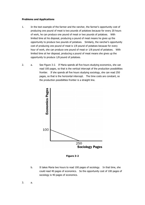
Problems and Applications1.In the text example of the farmer and the rancher, the farmer’s opportunity cost ofproducing one pound of meat is two pounds of potatoes because for every 20 hours of work, he can produce one pound of meat or two pounds of potatoes. Withlimited time at his disposal, producing a pound of meat means he gives up theopportunity to produce two pounds of potatoes. Similarly, the rancher’s opportunity cost of producing one pound of meat is 1/8 pound of potatoes because for everyhour of work, she can produce one pound of meat or 1/8 pound of potatoes. Withlimited time at her disposal, producing a pound of meat means she gives up theopportunity to produce 1/8 pound of potatoes.2. a.See Figure 3-2. If Maria spends all five hours studying economics, she canread 100 pages, so that is the vertical intercept of the production possibilitiesfrontier. If she spends all five hours studying sociology, she can read 250pages, so that is the horizontal intercept. The time costs are constant, sothe production possibilities frontier is a straight line.Figure 3-2b.It takes Maria two hours to read 100 pages of sociology. In that time, shecould read 40 pages of economics. So the opportunity cost of 100 pages ofsociology is 40 pages of economics.3. a.Workers needed to make:One Car One Ton of Grain U.S.1/41/10Japan1/41/5b.See Figure 3-3. With 100 million workers and four cars per worker, if eithereconomy were devoted completely to cars, it could make 400 million cars.Since a U.S. worker can produce 10 tons of grain, if the U.S. produced onlygrain it would produce 1,000 million tons. Since a Japanese worker canproduce 5 tons of grain, if Japan produced only grain it would produce 500million tons. These are the intercepts of the production possibilities frontiers shown in the figure. Note that since the tradeoff between cars and grain isconstant, the production possibilities frontier is a straight line.Figure 3-3c.Since a U.S. worker produces either 4 cars or 10 tons of grain, theopportunity cost of 1 car is 2½ tons of grain, which is 10 divided by 4.Since a Japanese worker produces either 4 cars or 5 tons of grain, theopportunity cost of 1 car is1 1/4 tons of grain, which is 5 divided by 4. Similarly, the U.S. opportunitycost of 1 ton of grain is 2/5 cars (4 divided by 10) and the Japaneseopportunity cost of 1 ton of grain is 4/5 cars (4 divided by 5). This gives the following table:Opportunity Cost of:1 Car (in terms of tons ofgrain given up)1 Ton of Grain (in termsof cars given up)U.S. 2 1/22/5Japan 1 1/44/5d.Neither country has an absolute advantage in producing cars, since they’reequally productive (the same output per worker); the U.S. has an absoluteadvantage in producing grain, since it’s more productive (greater output perworker).e.Japan has a comparative advantage in producing cars, since it has a loweropportunity cost in terms of grain given up. The U.S. has a comparativeadvantage in producing grain, since it has a lower opportunity cost in termsof cars given up.f.With half the workers in each country producing each of the goods, the U.S.would produce 200 million cars (that’s 50 million workers times 4 cars each)and 500 million tons of grain (50 million workers times 10 tons each).Japan would produce 200 million cars (50 million workers times 4 cars each)and 250 million tons of grain (50 million workers times 5 tons each).g.From any situation with no trade, in which each country is producing somecars and some grain, suppose the U.S. changed 1 worker from producingcars to producing grain. That worker would produce 4 fewer cars and 10additional tons of grain. Then suppose the U.S. offers to trade 7 tons ofgrain to Japan for 4 cars. The U.S. will do this because it values 4 cars at 10tons of grain, so it will be better off if the trade goes through. SupposeJapan changes 1 worker from producing grain to producing cars. Thatworker would produce 4 more cars and 5 fewer tons of grain. Japan willtake the trade because it values 4 cars at 5 tons of grain, so it will be betteroff. With the trade and the change of 1 worker in both the U.S. and Japan,each country gets the same amount of cars as before and both get additionaltons of grain (3 for the U.S. and 2 for Japan). Thus by trading and changingtheir production, both countries are better off.4. a.Pat’s opportunity cost of making a pizza is 1/2 gallon of root beer, since shecould brew 1/2 gallon in the time (2 hours) it takes her to make a pizza. Pathas an absolute advantage in making pizza since she can make one in twohours, while it takes Kris four hours. Kris’s opportunity cost of making apizza is 2/3 gallons of root beer, since she could brew 2/3 of a gallon in thetime (4 hours) it takes her to make a pizza. Since Pat’s opportunity cost ofmaking pizza is less than Kris’s, Pat has a comparative advantage in makingpizza.b.Since Pat has a comparative advantage in making pizza, she will make pizzaand exchange it for root beer that Kris makes.c.The highest price of pizza in terms of root beer that will make bothroommates better off is 2/3 gallons of root beer. If the price were higherthan that, then Kris would prefer making her own pizza (at an opportunitycost of 2/3 gallons of root beer) rather than trading for pizza that Pat makes.The lowest price of pizza in terms of root beer that will make bothroommates better off is 1/2 gallon of root beer. If the price were lower thanthat, then Pat would prefer making her own root beer (she can make 1/2gallon of root beer instead of making a pizza) rather than trading for rootbeer that Kris makes.5. a.Since a Canadian worker can make either two cars a year or 30 bushels ofwheat, the opportunity cost of a car is 15 bushels of wheat. Similarly, theopportunity cost of a bushel of wheat is 1/15 of a car. The opportunitycosts are the reciprocals of each other.b.See Figure 3-4. If all 10 million workers produce two cars each, theyproduce a total of 20 million cars, which is the vertical intercept of theproduction possibilities frontier. If all 10 million workers produce 30 bushelsof wheat each, they produce a total of 300 million bushels, which is thehorizontal intercept of the production possibilities frontier. Since thetradeoff between cars and wheat is always the same, the productionpossibilities frontier is a straight line.If Canada chooses to consume 10 million cars, it will need 5 million workersdevoted to car production. That leaves 5 million workers to produce wheat,who will produce a total of 150 million bushels (5 million workers times 30bushels per worker). This is shown as point A on Figure 3-4.c.If the United States buys 10 million cars from Canada and Canada continuesto consume 10 million cars, then Canada will need to produce a total of 20million cars. So Canada will be producing at the vertical intercept of theproduction possibilities frontier. But if Canada gets 20 bushels of wheat percar, it will be able to consume 200 million bushels of wheat, along with the10 million cars. This is shown as point B in the figure. Canada should acceptthe deal because it gets the same number of cars and 50 million morebushes of wheat.Figure 3-46.Though the professor could do both writing and data collection faster than thestudent (that is, he has an absolute advantage in both), his time is limited. If theprofessor’s comparative advantage is in writing, it makes sense for him to pay astudent to collect the data, since that’s the student’s comparative advantage.7. a.English workers have an absolute advantage over Scottish workers inproducing scones, since English workers produce more scones per hour (50vs. 40). Scottish workers have an absolute advantage over English workersin producing sweaters, since Scottish workers produce more sweaters perhour (2 vs. 1). Comparative advantage runs the same way. Englishworkers, who have an opportunity cost of 1/50 sweaters per scone (1sweater per hour divided by 50 scones per hour), have a comparativeadvantage in scone production over Scottish workers, who have anopportunity cost of 1/20 sweater per scone (2 sweaters per hour divided by40 scones per hour). Scottish workers, who have an opportunity cost of 20scones per sweater (40 scones per hour divided by 2 sweaters per hour),have a comparative advantage in sweater production over English workers,who have an opportunity cost of 50 scones per sweater (50 scones per hourdivided by 1 sweater per hour).b.If England and Scotland decide to trade, Scotland will produce sweaters andtrade them for scones produced in England. A trade with a price between20 and 50 scones per sweater will benefit both countries, as they’ll be gettingthe traded good at a lower price than their opportunity cost of producing thegood in their own country.c.Even if a Scottish worker produced just one sweater per hour, the countrieswould still gain from trade, because Scotland would still have a comparativeadvantage in producing sweaters. Its opportunity cost for sweaters wouldbe higher than before (40 scones per sweater, instead of 20 scones persweater before). But there are still gains from trade since England has ahigher opportunity cost (50 scones per sweater).8. a.Technological advance lowers the opportunity cost of producing meat for thefarmer. The opportunity cost of producing a point of meat was 2 pounds ofpotatoes; it’s now 1/5 pounds of potatoes. Thus the farmer’s opportunitycost of producing potatoes is now 5 pounds of meat. Since the rancher’sopportunity cost of producing potatoes is 8 pounds of meat, the farmer stillhas a comparative advantage in producing potatoes and the rancher still hasa comparative advantage in producing meat.b.Now the farmer won’t be willing to trade a pound of potatoes for 3 pounds ofmeat because if he produced one less pound of potatoes, he could produce 5more pounds of meat. So the trade would be bad for the farmer, as hewould then be consuming inside his production possibilities frontier.c.The farmer and rancher would now be willing to trade one pound of potatoesfor an amount between 5 and 8 pounds of meat, with the potatoes beingproduced by the farmer and the meat being produced by the rancher.9. a.With no trade, one pair of white socks trades for one pair of red socks inBoston, since productivity is the same for the two types of socks. The pricein Chicago is 2 pairs of red socks per pair of white socks.b.Boston has an absolute advantage in the production of both types of socks,since a worker in Boston produces more (3 pairs of socks per hour) than aworker in Chicago (2 pairs of red socks per hour or 1 pair of white socks perhour).Chicago has a comparative advantage in producing red socks, since theopportunity cost of producing a pair of red socks in Chicago is 1/2 pair ofwhite socks, while the opportunity cost of producing a pair of red socks inBoston is 1 pair of white socks. Boston has a comparative advantage inproducing white socks, since the opportunity cost of producing a pair ofwhite socks in Boston is 1 pair of red socks, while the opportunity cost ofproducing a pair of white socks in Chicago is 2 pairs of red socks.c.If they trade socks, Boston will produce white socks for export, since it hasthe comparative advantage in white socks, while Chicago produces red socksfor export, which is Chicago’s comparative advantage.d.Trade can occur at any price between 1 and 2 pairs of red socks per pair ofwhite socks. At a price lower than 1 pair of red socks per pair of whitesocks, Boston will choose to produce its own red socks (at a cost of 1 pair ofred socks per pair of white socks) instead of buying them from Chicago. Ata price higher than 2 pairs of red socks per pair of white socks, Chicago willchoose to produce its own white socks (at a cost of 2 pairs of red socks perpair of white socks) instead of buying them from Boston.10. a.The cost of all goods is lower in Germany than in France in the sense that allgoods can be produced with fewer worker hours.b.The cost of any good for which France has a comparative advantage is lowerin France than in Germany. Though Germany produces all goods with lesslabor, that labor is more valuable. So the cost of production, in terms ofopportunity cost, will be lower in France for some goods.c.Trade between Germany and France will benefit both countries. For eachgood in which it has a comparative advantage, each country should producemore goods than it consumes, trading the rest to the other country. Totalconsumption will be higher in both countries as a result.11. a.True; two countries can achieve gains from trade even if one of the countrieshas an absolute advantage in the production of all goods. All that’snecessary is that each country have a comparative advantage in some good.b.False; it is not true that some people have a comparative advantage ineverything they do. In fact, no one can have a comparative advantage ineverything. Comparative advantage reflects the opportunity cost of onegood or activity in terms of another. If you have a comparative advantagein one thing, you must have a comparative disadvantage in the other thing.c.False; it is not true that if a trade is good for one person, it can’t be good forthe other one. Trades can and do benefit both sides especially tradesbased on comparative advantage. If both sides didn’t benefit, trades wouldnever occur.。
曼昆《宏观经济学》第9版章节习题精编详解(经济增长Ⅱ:技术、经验和政策)【圣才出品】

曼昆《宏观经济学》(第9版)章节习题精编详解第3篇增长理论:超长期中的经济第9章经济增长Ⅱ:技术、经验和政策一、概念题1.劳动效率(efficiency of labor)答:劳动效率是指单位劳动时间的产出水平,反映了社会对生产方法的掌握和熟练程度。
当可获得的技术改进时,劳动效率会提高。
当劳动力的健康、教育或技能得到改善时,劳动效率也会提高。
在索洛模型中,劳动效率(E)是表示技术进步的变量,反映了索洛模型劳动扩张型技术进步的思想:技术进步提高了劳动效率,就像增加了参与生产的劳动力数量一样,所以在生产函数中的劳动力数量上乘以一个劳动效率变量,形成了有效工人概念,这使得索洛模型在稳态分析中纳入了外生的技术进步。
2.劳动改善型技术进步(labor-augmenting technological progress)答:劳动改善型技术进步是指技术进步提高了劳动效率,就像增加了参与生产的劳动力数量一样,所以在生产函数中的劳动力数量上乘以一个劳动效率变量,以反映外生技术进步对经济增长的影响。
劳动改善型技术进步实际上认为技术进步是通过提高劳动效率而影响经济增长的。
它的引入形成了有效工人的概念,从而使得索洛模型能够以单位有效工人的资本和产量来进行稳定状态研究。
3.内生增长理论(endogenous growth theory)答:内生增长理论是用规模收益递增和内生技术进步来说明一个国家长期经济增长和各国增长率差异的一种经济理论,其重要特征就是试图使增长率内生化。
根据其依赖的基本假定条件的差异,可以将内生增长理论分为完全竞争条件下的内生增长模型和垄断竞争条件下的内生增长模型。
按照完全竞争条件下的内生增长模型,使稳定增长率内生化的两条基本途径就是:①将技术进步率内生化;②如果可以被积累的生产要素有固定报酬,那么可以通过某种方式使稳态增长率受要素的积累影响。
内生增长理论是抛弃了索洛模型外生技术进步的假设,以更好地研究技术进步与经济增长之间的关系的理论。
国际经济学第九版英文课后答案第3单元
国际经济学第九版英文课后答案第3单元*CHAPTER 3(Core Chapter)THE STANDARD THEORY OF INTERNATIONAL TRADE OUTLINE3.1 Introduction3.2 The Production Frontier with Increasing Costs3.2a Illustration of Increasing Costs3.2b The Marginal Rate of Transformation3.2c Reason for Increasing Opportunity Costs and Different Production Frontiers3.3 Community Indifference Curves3.3a Illustration of Community Indifference Curves3.3b The Marginal Rate of Substitution3.3c Some Difficulties with Community Indifference Curves3.4 Equilibrium in Isolation3.4a Illustration of Equilibrium in Isolation3.4b Equilibrium Relative Commodity Prices and Comparative AdvantageCase 3-1: Revealed Comparative Advantage of the United States,the European Union, and Japan3.5 The Basis for and the Gains from Trade with Increasing Costs3.5a Illustration of the Basis for and the Gains from Trade with Increasing Costs3.5b Equilibrium Relative Commodity Prices with Trade3.5c Incomplete SpecializationCase Study 3-2: Specialization and Export Concentration inSelected Countries3.5d Small Country Case with Increasing Costs3.5e The Gains from Exchange and from SpecializationCase Study 3-3: Job Losses in High U.S. Import-Competing IndustriesCase Study 3-4: International Trade and Deindustrialization in the United States,the European Union, and Japan3.6 Trade Based on Differences in TastesAPPENDIX: A3.1 Production Functions, Isoquants, Isocosts and EquilibriumA3.2 Production Theory with Two Nations, Two Commodities and Two FactorsA3.3 Derivation of the Edgeworth Box Diagram and Production FrontiersA3.4 Some Important ConclusionsKey TermsIncreasing opportunity costs Revealed comparative advantage Marginal rate of transformation (MRT) Equilibrium relative commodity price with tradeCommunity indifference curves Incomplete specialization Marginal rate of substitution (MRS) Gains from exchange Autarky Gains from specializationEquilibrium relative commodity price in isolation Deindustrialization Lecture Guide1. In the first lecture of Chapter 3, I would cover Sections 1, 2, and3. Section 2 can becovered quickly, except for 2b, which requires careful explanation because of its subsequentimportance. Careful explanation is also required for 3b. I would assign Problems 1 and 2.2. In the second lecture, I would cover Sections 4, 5a, and 5b. Thisis the basic trade modeland it is essential for the student to master it completely. To this end, I would assign andgrade Problems 3 and 4.3. In the third lecture, I would cover the remainder of the chapter.The topics here representelaborations of the basic trade model. I would assign problems 5, 6, and 7 and go overproblem 7 in class even though its answer is also in the back of the book. I would make theAppendices optional for those students in the class who have had intermediate micro theory.Answer to Problems1. a) See Figure 1.b) The slope of the transformation curve increases as the nationproduces more of X anddecreases as the nation produces more of Y. These reflect increasing opportunity costs asthe nation produces more of X or Y.2. a) See Figure 2.We have drawn community indifference curves as downward or negatively sloped becauseas the community consumes more of X it will have to give up some of Y to remain onthe same indifference curve.b)The slope measures how much of Y the nation can give up byconsuming one more unitof X and still remain at the same level of satisfaction; the slope declines because the moreof X and the less of Y the nation is left with, the less satisfaction it receives fromadditional units of X and the more satisfaction it receives from each retained unit of Y.c) III > II to the right of the intersection, while II > III to the left.This is inconsistent because an indifference curve should show a given level of satisfaction.Thus, indifference curves cannot cross.3. a) See Figure 3 on page 22.b) Nation 1 has a comparative advantage in X and Nation 2 in Y.c) If the relative commodity price line has equal slope in both nations.4. a) See Figure 4.b) Nation 1 gains by the amount by which point E is to the right andabove point A andNation 2 by the excess of E' over A'. Nation 1 gains more from trade because the relativeprice of X with trade differs more from its pretrade price than for Nation 2.5. a) See Figure 5. In Figure 5, S refers to Nation 1's supplycurve of exports of commodity X, while D refers to Nation 2's demand curve for Nation 1's exports of commodity X. D and S intersect at point E, determining the equilibrium P B=Px/Py=1 and the equilibrium quantity of exports of 60X.b) At Px/Py=1 1/2 there is an excess supply of exports of R'R=30Xand Px/Py falls towardequilibrium Px/Py=1.c) At Px/Py=1/2, there is an excess demand of exports of HH'=80X and Px/Py risestoward Px/Py=1.6. The Figure in Problem 5 is consistent with Figure 3-4 in the text.From the left panel ofFigure 3-4, we see that Nation 1 supplies no exports of commodity X at Px/Py=1/4 (pointA). This corresponds with the vertical or price intercept of Nation 1's supply curve ofexports of commodity X (point A).The left panel of Figure 3-4 also shows that at Px/Py=1, Nation 1 is willing to export 60X(point E). The same is shown by Nation 1's supply curve of exports of commodity X.The other points on Nation 1's supply curve of exports in the figure of Problem 5 can alsobe derived from the left panel of Figure 3-4, but this is shown in Chapter 4 with offercurves.Nation 2's demand curve for Nation 1's exports ofcommodity X could be derived from theright panel of Figure 3-4, as shown in Chapter 4. What is important isthat we can use theD and S figure in Problem 5 to explain why the equilibrium relative commodity price withtrade is Px/Py=1 and why the equilibrium quantity traded of commodity X is 60 units inFigure 3-4.7. See Figure 6 on page 24.The small nation will move from A to B in production, exports X in exchange for Y so asto reach point E > A.8. a) The small nation specializes in the production of commodityX only until its opportunitycost and relative price of X equals P W. This usually occurs before the small nation hasbecome completely specialized in production.b) Under constant costs, specialization is always complete for the small nation.9. a) See Figure 7.b) See Figure 8.10. If the two community indifference curves had also been identical in Problem 9 the relativecommodity prices would also have been the same in both nations in the absence of trade andno mutually beneficial trade would be possible11. If production frontiers are identical and the communityindifference curves different in thetwo nations, but we have constant opportunity costs, there would be no mutually beneficialtrade possible between the two nations12. See Figure 1113. It is true that Mexico's wages are much lower than U.S. wages (about one fifth), but laborproductivity is much higher in the United States and so labor costs are not necessarilyhigher than in Mexico. In any event, trade can still be based on comparative advantage.App. 1. See Figure 12Commodity X is the L-intensive commodity in Nation 2 (as in Nation 1) because the production contract curve bulges toward the L- axis or is everywhere to the left of the diagonal.App. 2. Since L and K are released from the production of X in a higher ratio than are absorbed in the production of Y, wages fall in Nation 2. This leads to the substitution of L for K in the production of X and Y, so that the K/L ratio falls in the production of both commodities.Multiple-Choice Questions1. A production frontier that is concave from the origin indicates that thenation incursincreasing opportunity costs in the production of:a. commodity X onlyb. commodity Y only*c. both commoditiesd. neither commodity2. The marginal rate of transformation (MRT) of X for Y refers to:a. the amount of Y that a nation must give up to produce each additional unit of Xb. the opportunity cost of Xc. the absolute slope of the production frontier at the point of production*d. all of the above3. Which of the following is not a reason for increasing opportunity costs:*a. technology differs among nationsb. factors of production are not homogeneousc. factors of production are not used in the same fixed proportion in the production of all commoditiesd. for the nation to produce more of a commodity, it must use resources that are less and less suited in the production of the commodity4. Community indifference curves:a. are negatively slopedb. are convex to the originc. should not cross*d. all of the above5. The marginal rate of substitution (MRS) of X for Y in consumption refers to the:a. amount of X that a nation must give up for one extra unit of Y and still remain on the same indifference curve*b. amount of Y that a nation must give up for one extra unit of X and still remain on the same indifference curvec. amount of X that a nation must give up for one extra unit of Y to reach a higher indifference curved. amount of Y that a nation must give up for one extra unit of X to reach a higher indifference curve6. Which of the following statements is true with respect to the MRS of X for Y?a. It is given by the absolute slope of the indifference curveb. declines as the nation moves down an indifference curvec. rises as the nation moves up an indifference curve*d. all of the above7. Which of the following statements about community indifference curves is true?a. They are entirely unrelated to individuals' community indifference curvesb. they cross, they cannot be used in the analysis*c. the problems arising from intersecting community indifference curves can be overcome by the application of the compensation principled. all of the above.8. Which of the following is not true for a nation that is in equilibrium in isolation?*a. It consumes inside its production frontierb. it reaches the highest indifference curve possible with its production frontierc. the indifference curve is tangent to the nation's production frontierd. MRT of X for Y equals MRS of X for Y, and they are equal to Px/Py9. If the internal Px/Py is lower in nation 1 than in nation 2 without trade:a. nation 1 has a comparative advantage in commodity Yb. nation 2 has a comparative advantage in commodity X*c. nation 2 has a comparative advantage in commodity Yd. none of the above10. Nation 1's share of the gains from trade will be greater:a. the greater is nation 1's demand for nation 2's exports*b. the closer Px/Py with trade settles to nation 2's pretrade Px/Pyc. the weaker is nation 2's demand for nation 1's exportsd. the closer Px/Py with trade settles to nation 1's pretrade Px/Py11. If Px/Py exceeds the equilibrium relative Px/Py with tradea. the nation exporting commodity X will want to export more of X than at equilibriumb. the nation importing commodity X will want to import less of X than at equilibriumc. Px/Py will fall toward the equilibrium Px/Py*d. all of the above12. With free trade under increasing costs:a. neither nation will specialize completely in productionb. at least one nation will consume above its production frontierc. a small nation will always gain from trade*d. all of the above13. Which of the following statements is false?a.The gains from trade can be broken down into the gains from exchange and the gains from specializationb. gains from exchange result even without specialization*c. gains from specialization result even without exchanged. none of the above14. The gains from exchange with respect to the gains fromspecialization are always:a. greaterb. smallerc. equal*d. we cannot say without additional information15. Mutually beneficial trade cannot occur if production frontiers are:a. equal but tastes are notb. different but tastes are the samec. different and tastes are also different*d. the same and tastes are also the same.。
曼昆微观经济学课后练习英文答案完整版

曼昆微观经济学课后练习英文答案集团标准化办公室:[VV986T-J682P28-JP266L8-68PNN]the link between buyers’ willingness to pay for a good and the demandcurve.how to define and measure consumer surplus.the link between sellers’ costs of producing a good and the supply curve.how to define and measure producer surplus.that the equilibrium of supply and demand maximizes total surplus in amarket.CONTEXT AND PURPOSE:Chapter 7 is the first chapter in a three-chapter sequence on welfare economics and market efficiency. Chapter 7 employs the supply and demand model to develop consumer surplus and producer surplus as a measure of welfare and market efficiency. These concepts are then utilized in Chapters 8 and 9 to determine the winners and losers from taxation and restrictions on international trade.The purpose of Chapter 7 is to develop welfare economics—the study of how the allocation of resources affects economic well-being. Chapters 4 through 6 employed supply and demand in a positive framework, which focused on the question, “What is the equilibrium price and quantity in a market” This chapter now addresses the normative question, “Is the equilibrium price and quantity in a market the best possible solution to the resource allocation problem, or is it simply the price and quantity that balance supply and demand” Students will discover that under most circumstances the equilibrium price and quantity is also the one that maximizes welfare.KEY POINTS:Consumer surplus equals buyers’ willingness to pay for a good minus the amount they actually pay for it, and it measures the benefit buyers get from participating in a market. Consumer surplus can be computed by finding the area below the demand curve and above the price.Producer surplus equals the amount sellers receive for their goods minus their costs of production, and it measures the benefit sellers get from participating in a market. Producer surplus can be computed by finding the area below the price and above the supply curve.An allocation of resources that maximizes the sum of consumer and producer surplus is said to be efficient. Policymakers are often concerned with the efficiency, as well as the equality, of economic outcomes.The equilibrium of supply and demand maximizes the sum of consumer andproducer surplus. That is, the invisible hand of the marketplace leadsbuyers and sellers to allocate resources efficiently.Markets do not allocate resources efficiently in the presence of market failures such as market power or externalities.CHAPTER OUTLINE:I. Definition of welfare economics: the study of how the allocation of resources affects economic well-being.A. Willingness to Pay1. Definition of willingness to pay: the maximum amount that a buyer will pay for a good.2. Example: You are auctioning a mint-condition recording of Elvis Presley’s first album. Four buyers show up. Their willingness to pay is as follows:If the bidding goes to slightly higher than $80, all buyersdrop out except for John. Because John is willing to paymore than he has to for the album, he derives some benefitfrom participating in the market.3. Definition of consumer surplus: the amount a buyer is willing to payfor a good minus the amount the buyer actually pays for it.4. Note that if you had more than one copy of the album, the price in the auction would end up being lower (a little over $70 in the case of two albums) and both John and Paul would gain consumer surplus.B. Using the Demand Curve to Measure Consumer Surplus1. We can use the information on willingness to pay to derive a demandmarginal buyer . Because the demand curve shows the buyers’ willingness to pay, we can use the demand curve to measure c onsumer surplus.C. How a Lower Price Raises Consumer Surplussurplus because they are paying less for the product than before (area A on the graph).b. Because the price is now lower, some new buyers will enter the market and receive consumer surplus on these additional units of output purchased (area B on the graph).D. What Does Consumer Surplus Measure?1. Remember that consumer surplus is the difference between the amount that buyers are willing to pay for a good and the price that they actually pay.2. Thus, it measures the benefit that consumers receive from the good as the buyers themselves perceive it.III. Producer SurplusA. Cost and the Willingness to Sell1. Definition of cost: the value of everything a seller must give up to produce a good .2. Example: You want to hire someone to paint your house. You accept bidsfor the work from four sellers. Each painter is willing to work if the priceyou will pay exceeds her opportunity cost. (Note that this opportunity costthus represents willingness to sell.) The costs are:sellers will drop out except for Grandma. Because Grandma receives more than she would require to paint the house, she derives some benefit from producing in the market.4. Definition of producer surplus: the amount a seller is paid for a good minus the seller’s cost of providing it.5. Note that if you had more than one house to paint, the price in the auction would end up being higher (a little under $800 in the case of two houses) and both Grandma and Georgia would gain producer surplus.ALTERNATIVE CLASSROOM EXAMPLE:Review the material on price ceilings from Chapter 6. Redraw themarket for two-bedroom apartments in your town. Draw in a priceceiling below the equilibrium price.Then go through:consumer surplus before the price ceiling is put into place. consumer surplus after the price ceiling is put into place. You will need to take some time to explain the relationship between the producers’ willingness to sell and the cost of producing the good. The relationship between cost and the supply curve is not as apparent as the relationship between the It is important to stress that consumer surplus is measured inmonetary terms. Consumer surplus gives us a way to place amonetary cost on inefficient market outcomes (due to governmentB. Using the Supply Curve to Measure Producer Surplus1. We can use the information on cost (willingness to sell) to derive a2.the cost of the marginal seller. Because the supply curve shows the sellers’ cost (willingness to sell), we can use the supply curve to measure producer surplus.C. How a Higher Price Raises Producer Surplussurplus because they are receiving more for the product than before (area C on the graph).b. Because the price is now higher, some new sellers will enter the market and receive producer surplus on these additional units of output sold (area D on the graph).D. Producer surplus is used to measure the economic well-being of producers,ALTERNATIVE CLASSROOM EXAMPLE:Review the material on price floors from Chapter 6. Redraw the marketfor an agricultural product such as corn. Draw in a price supportabove the equilibrium price.Then go through:producer surplus before the price support is put in place.producer surplus after the price support is put in place.Make sure that you discuss the cost of the price support tomuch like consumer surplus is used to measure the economic well-being of consumers.IV. Market EfficiencyA. The Benevolent Social Planner1. The economic well-being of everyone in society can be measured by total surplus, which is the sum of consumer surplus and producer surplus:Total Surplus = Consumer Surplus + Producer SurplusTotal Surplus = (Value to Buyers – Amount Paid byBuyers) +(Amount Received by Sellers – Cost to Sellers)Because the Amount Paid by Buyers = Amount Received bySellers:2. Definition of efficiency: the property of a resource allocation of maximizing the total surplus received by all members of society .3. Definition of equality: the property of distributing economicprosperity uniformly the members of society .a. Buyers who value the product more than the equilibrium price will purchase the product; those who do not, will not purchase the product. Inother words, the free market allocates the supply of a good to the buyers who value it most highly, as measured by their willingness to pay.b. Sellers whose costs are lower than the equilibrium price will produce the product; those whose costs are higher, will not produce the product. Inother words, the free market allocates the demand for goods to the sellers who can produce it at the lowest cost.value of the product to the marginal buyer is greater than the cost to the marginal seller so total surplus would rise if output increases.Pretty Woman, Chapter 6. Vivien (Julia Roberts) and Edward(Richard Gere) negotiate a price. Afterward, Vivien reveals shewould have accepted a lower price, while Edward admits he wouldhave paid more. If you have done a good job of introducingconsumer and producer surplus, you will see the light bulbs gob. At any quantity of output greater than the equilibrium quantity, the value of the product to the marginal buyer is less than the cost to the marginal seller so total surplus would rise if output decreases.3. Note that this is one of the reasons that economists believe Principle #6: Markets are usually a good way to organize economic activity.C. In the News: Ticket Scalping1. Ticket scalping is an example of how markets work to achieve anefficient outcome.2. This article from The Boston Globe describes economist Chip Case’sexperience with ticket scalping.D. Case Study: Should There Be a Market in Organs?1. As a matter of public policy, people are not allowed to sell their organs.a. In essence, this means that there is a price ceiling on organs of $0.b. This has led to a shortage of organs.2. The creation of a market for organs would lead to a more efficientallocation of resources, but critics worry about the equity of a market system for organs.V. Market Efficiency and Market FailureA. To conclude that markets are efficient, we made several assumptions about how markets worked.1. Perfectly competitive markets.2. No externalities.B. When these assumptions do not hold, the market equilibrium may not be efficient.C. When markets fail, public policy can potentially remedy the situation. SOLUTIONS TO TEXT PROBLEMS:Quick Quizzes1. Figure 1 shows the demand curve for turkey. The price of turkey is P 1and the consumer surplus that results from that price is denoted CS. Consumer surplus is the amount a buyer is willing to pay for a good minus the amount the buyer actually pays for it. It measures the benefit to buyers ofparticipating in a market.Figure 1 Figure 22. Figure 2 shows the supply curve for turkey. The price of turkey is P 1and the producer surplus that results from that price is denoted PS. Producer surplus is the amount sellers are paid for a good minus the sellers’ cost of providing it (measured by the supply curve). It measures the benefit to sellers of participating in a market.It would be a good idea to remind students that there are circumstances when the market process does not lead to the most efficient outcome. Examples include situations such as when a firm (or buyer) has market power over price or when there areFigure 33. Figure 3 shows the supply and demand for turkey. The price of turkey is P, consumer surplus is CS, and producer surplus is PS. Producing more turkeys 1than the equilibrium quantity would lower total surplus because the value to the marginal buyer would be lower than the cost to the marginal seller on those additional units.Questions for Review1. The price a buyer is willing to pay, consumer surplus, and the demand curve are all closely related. The height of the demand curve represents the willingness to pay of the buyers. Consumer surplus is the area below the demand curve and above the price, which equals the price that each buyer is willing to pay minus the price actually paid.2. Sellers' costs, producer surplus, and the supply curve are all closely related. The height of the supply curve represents the costs of the sellers. Producer surplus is the area below the price and above the supply curve, which equals the price received minus each seller's costs of producing the good.Figure 43. Figure 4 shows producer and consumer surplus in a supply-and-demand diagram.4. An allocation of resources is efficient if it maximizes total surplus, the sum of consumer surplus and producer surplus. But efficiency may not be the only goal of economic policymakers; they may also be concerned about equitythe fairness of the distribution of well-being.5. The invisible hand of the marketplace guides the self-interest of buyers and sellers into promoting general economic well-being. Despite decentralized decision making and self-interested decision makers, free markets often lead to an efficient outcome.6. Two types of market failure are market power and externalities. Market power may cause market outcomes to be inefficient because firms may cause price and quantity to differ from the levels they would be under perfect competition, which keeps total surplus from being maximized. Externalities are side effects that are not taken into account by buyers and sellers. As a result, the free market does not maximize total surplus.Problems and Applications1. a. Consumer surplus is equal to willingness to pay minus the price paid. Therefore, Melissa’s willingness to pay must be $200 ($120 + $80).b. Her consumer surplus at a price of $90 would be $200 $90 = $110.c. If the price of an iPod was $250, Melissa would not have purchased one because the price is greater than her willingness to pay. Therefore, she would receive no consumer surplus.2. If an early freeze in California sours the lemon crop, the supply curve for lemons shifts to the left, as shown in Figure 5. The result is a rise in the price of lemons and a decline in consumer surplus from A + B + C to just A. So consumer surplus declines by the amount B + C.Figure 5 Figure 6In the market for lemonade, the higher cost of lemons reduces the supply of lemonade, as shown in Figure 6. The result is a rise in the price of lemonade and a decline in consumer surplus from D + E + F to just D, a loss of E + F. Note that an event that affects consumer surplus in one market oftenhas effects on consumer surplus in other markets.3. A rise in the demand for French bread leads to an increase in producer surplus in the market for French bread, as shown in Figure 7. The shift of the demand curve leads to an increased price, which increases producer surplusfrom area A to area A + B + C.Figure 7The increased quantity of French bread being sold increases the demandfor flour, as shown in Figure 8. As a result, the price of flour rises, increasing producer surplus from area D to D + E + F. Note that an event that affects producer surplus in one market leads to effects on producer surplus in related markets.Figure 84. a.Figure 9b. When the price of a bottle of water is $4, Bert buys two bottles of water. His consumer surplus is shown as area A in the figure. He values hisfirst bottle of water at $7, but pays only $4 for it, so has consumer surplus of $3. He values his second bottle of water at $5, but pays only $4 for it, so has consumer surplus of $1. Thus Bert’s total consumer surplus is $3 + $1 = $4, which is the area of A in the figure.c. When the price of a bottle of water falls from $4 to $2, Bert buys three bottles of water, an increase of one. His consumer surplus consists of both areas A and B in the figure, an increase in the amount of area B. He gets consumer surplus of $5 from the first bottle ($7 value minus $2 price), $3from the second bottle ($5 value minus $2 price), and $1 from the third bottle ($3 value minus $2 price), for a total consumer surplus of $9. Thus consumer surplus rises by $5 (which is the size of area B) when the price of a bottle of water falls from $4 to $2.5. a.Figure 10b. When the price of a bottle of water is $4, Ernie sells two bottles of water. His producer surplus is shown as area A in the figure. He receives $4 for his first bottle of water, but it costs only $1 to produce, so Ernie has producer surplus of $3. He also receives $4 for his second bottle of water, which costs $3 to produce, so he has producer surplus of $1. Thus Ernie’s total producer surplus is $3 + $1 = $4, which is the area of A in the figure.c. When the price of a bottle of water rises from $4 to $6, Ernie sells three bottles of water, an increase of one. His producer surplus consists of both areas A and B in the figure, an increase by the amount of area B. He gets producer surplus of $5 from the first bottle ($6 price minus $1 cost), $3 from the second bottle ($6 price minus $3 cost), and $1 from the third bottle ($6 price minus $5 price), for a total producer surplus of $9. Thus producer surplus rises by $5 (which is the size of area B) when the price of a bottle of water rises from $4 to $6.6. a. From Ernie’s supply schedule and Bert’s demand schedule, thean equilibrium quantity of two.b. At a price of $4, consumer surplus is $4 and producer surplus is $4, as shown in Problems 3 and 4 above. Total surplus is $4 + $4 = $8.c. If Ernie produced one less bottle, his producer surplus would decline to $3, as shown in Problem 4 above. If Bert consumed one less bottle, hisconsumer surplus would decline to $3, as shown in Problem 3 above. So total surplus would decline to $3 + $3 = $6.d. If Ernie produced one additional bottle of water, his cost would be $5, but the price is only $4, so his producer surplus would decline by $1. If Bert consumed one additional bottle of water, his value would be $3, but the price is $4, so his consumer surplus would decline by $1. So total surplus declines by $1 + $1 = $2.7. a. The effect of falling production costs in the market for stereos results in a shift to the right in the supply curve, as shown in Figure 11. As a result, the equilibrium price of stereos declines and the equilibriumquantity increases.Figure 11b. The decline in the price of stereos increases consumer surplus from area A to A + B + C + D, an increase in the amount B + C + D. Prior to the shift in supply, producer surplus was areas B + E (the area above the supply curve and below the price). After the shift in supply, producer surplus is areas E + F + G. So producer surplus changes by the amount F + G – B, which may be positive or negative. The increase in quantity increases producer surplus, while the decline in the price reduces producer surplus. Because consumer surplus rises by B + C + D and producer surplus rises by F + G – B, total surplus rises by C + D + F + G.c. If the supply of stereos is very elastic, then the shift of the supply curve benefits consumers most. To take the most dramatic case, suppose the supply curve were horizontal, as shown in Figure 12. Then there is no producer surplus at all. Consumers capture all the benefits of falling production costs, with consumer surplus rising from area A to area A + B.Figure 128. Figure 13 shows supply and demand curves for haircuts. Supply equals demand at a quantity of three haircuts and a price between $4 and $5. Firms A, C, and D should cut the hair of Ellen, Jerry, and Phil. Oprah’s willingnessto pay is too low and firm B’s costs are too high, so they do not participate. The maximum total surplus is the area between the demand and supply curves, which totals $11 ($8 value minus $2 cost for the first haircut, plus $7 value minus $3 cost for the second, plus $5 value minus $4 cost for the third).Figure 139. a. The effect of falling production costs in the market for computers results in a shift to the right in the supply curve, as shown in Figure 14. As a result, the equilibrium price of computers declines and the equilibrium quantity increases. The decline in the price of computers increases consumer surplus from area A to A + B + C + D, an increase in the amount B + C + D.Figure 14 Figure 15Prior to the shift in supply, producer surplus was areas B + E(the area above the supply curve and below the price). After theshift in supply, producer surplus is areas E + F + G. So producersurplus changes by the amount F + G – B, which may be positive ornegative. The increase in quantity increases producer surplus,while the decline in the price reduces producer surplus. Becauseconsumer surplus rises by B + C + D and producer surplus rises byF +G – B, total surplus rises by C + D + F + G.b. Because typewriters are substitutes for computers, the decline in the price of computers means that people substitute computers for typewriters, shifting the demand for typewriters to the left, as shown in Figure 15. The result is a decline in both the equilibrium price and equilibrium quantity of typewriters. Consumer surplus in the typewriter market changes from area A + B to A + C, a net change of C – B. Producer surplus changes from area C + D + E to area E, a net loss of C + D. Typewriter producers are sad about technological advances in computers because their producer surplus declines.c. Because software and computers are complements, the decline in the price and increase in the quantity of computers means that the demand for software increases, shifting the demand for software to the right, as shown in Figure 16. The result is an increase in both the price and quantity of software. Consumer surplus in the software market changes from B + C to A + B, a net change of A – C. Producer surplus changes from E to C + D + E, an increase of C + D, so software producers should be happy about the technological progress in computers.Figure 16d. Yes, this analysis helps explain why Bill Gates is one the world’s richest people, because his company produces a lot of software that is a complement with computers and there has been tremendous technological advance in computers.10. a. With Provider A, the cost of an extra minute is $0. WithProvider B, the cost of an extra minute is $1.b. With Provider A, my friend will purchase 150 minutes [= 150 –(50)(0)]. With Provider B, my friend would purchase 100 minutes [=150 – (50)(1)].c. With Provider A, he would pay $120. The cost would be $100 with Provider B.Figure 17d. Figure 17 shows the friend’s demand. With Provider A, he buys 150minutes and his consumer surplus is equal to (1/2)(3)(150) – 120= 105. With Provider B, his consumer surplus is equal to(1/2)(2)(100) = 100.e. I would recommend Provider A because he receives greater consumer surplus.11. a. Figure 18 illustrates the demand for medical care. If each procedure has a price of $100, quantity demanded will be Q1 procedures.Figure 18b. If consumers pay only $20 per procedure, the quantity demanded will be Qprocedures. Because the cost to society is $100, the number of procedures 2performed is too large to maximize total surplus. The quantity that maximizes total surplus is Q1 procedures, which is less than Q2.c. The use of medical care is excessive in the sense that consumers get procedures whose value is less than the cost of producing them. As a result, the economy’s total surplus is reduced.d. To prevent this excessive use, the consumer must bear the marginal cost of the procedure. But this would require eliminating insurance. Another possibility would be that the insurance company, which pays most of the marginal cost of the procedure ($80, in this case) could decide whether the procedure should be performed. But the insurance company does not get the benefits of the procedure, so its decisions may not reflect the value to the consumer.。
曼昆宏观经济经济学第九版英文原版复习资料3

Answers to Textbook Questions and ProblemsCHAPTER3 National Income: Where It Comes From and Where It GoesQuestions for Review1. The factors of production and the production technology determine the amount of output an economycan produce. The factors of production are the inputs used to produce goods and services: the most important factors are capital and labor. The production technology determines how much output can be produced from any given amounts of these inputs. An increase in one of the factors of production or an improvement in technology leads to an increase in the economy’s output.2. When a firm decides how much of a factor of production to hire or demand, it considers how thisdecision affects profits. For example, hiring an extra unit of labor increases output and thereforeincreases revenue; the firm compares this additional revenue to the additional cost from the higher wage bill. The additional revenue the firm receives depends on the marginal product of labor (MPL) and the price of the good produced (P). An additional unit of labor produces MPL units of additional output, which sells for P dollars per unit. Therefore, the additional revenue to the firm is P ⨯MPL. The cost of hiring the additional unit of labor is the wage W. Thus, this hiring decision has the following effect on profits:ΔProfit= ΔRevenue –ΔCost= (P ⨯MPL) –W.If the additional revenue, P ⨯MPL, exceeds the cost (W) of hiring the additional unit of labor, then profit increases. The firm will hire labor until it is no longer profitable to do so—that is, until the MPL falls to the point where the change in profit is zero. In the equation above, the firm hires labor until ΔP rofit = 0, which is when (P ⨯MPL) = W.This condition can be rewritten as:MPL = W/P.Therefore, a competitive profit-maximizing firm hires labor until the marginal product of labor equals the real wage. The same logic applies to the firm’s decision regarding how much capital to hire: the firm will hire capital until the marginal product of capital equals the real rental price.3. A production function has constant returns to scale if an equal percentage increase in all factors ofproduction causes an increase in output of the same percentage. For example, if a firm increases its use of capital and labor by 50 percent, and output increases by 50 percent, then the production function has constant returns to scale.If the production function has constant returns to scale, then total income (or equivalently, total output) in an economy of competitive profit-maximizing firms is divided between the return to labor, MPL ⨯L, and the return to capital, MPK ⨯K. That is, under constant returns to scale, economic profit is zero.4. A Cobb–Douglas production function has the form F(K,L) = AKαL1–α. The text showed that theparameter αgives capital’s share of income. So if capital earns one-fourth of total income, then α=0.25. Hence, F(K,L) = AK0.25L0.75.5. Consumption depends positively on disposable income—i.e. the amount of income after all taxes havebeen paid. Higher disposable income means higher consumption.The quantity of investment goods demanded depends negatively on the real interest rate. For an investment to be profitable, its return must be greater than its cost. Because the real interest ratemeasures the cost of funds, a higher real interest rate makes it more costly to invest, so the demand for investment goods falls.6. Government purchases are a measure of the value of goods and services purchased directly by thegovernment. For example, the government buys missiles and tanks, builds roads, and provides services such as air traffic control. All of these activities are part of GDP. Transfer payments are government payments to individuals that are not in exchange for goods or services. They are the opposite of taxes: taxes reduce household disposable income, whereas transfer payments increase it. Examples of transfer payments include Social Security payments to the elderly, unemployment insurance, and veterans’ benefits.7. Consumption, investment, and government purchases determine demand for the economy’s output,whereas the factors of production and the production function determine the supply of output. The real interest rate adjusts to ensure that the demand for the ec onomy’s goods equals the supply. At theequilibrium interest rate, the demand for goods and services equals the supply.8. When the government increases taxes, disposable income falls, and therefore consumption falls as well.The decrease in consumption equals the amount that taxes increase multiplied by the marginalpropensity to consume (MPC). The higher the MPC is, the greater is the negative effect of the tax increase on consumption. Because output is fixed by the factors of production and the production technology, and government purchases have not changed, the decrease in consumption must be offset by an increase in investment. For investment to rise, the real interest rate must fall. Therefore, a tax increase leads to a decrease in consumption, an increase in investment, and a fall in the real interest rate.Problems and Applications1. a. According to the neoclassical theory of distribution, the real wage equals the marginal product oflabor. Because of diminishing returns to labor, an increase in the labor force causes the marginalproduct of labor to fall. Hence, the real wage falls.Given a Cobb–Douglas production function, the increase in the labor force will increase the marginal product of capital and will increase the real rental price of capital. With more workers,the capital will be used more intensively and will be more productive.b. The real rental price equals the marginal product of capital. If an earthquake destroys some of thecapital stock (yet miraculously does not kill anyone and lower the labor force), the marginalproduct of capital rises and, hence, the real rental price rises.Given a Cobb–Douglas production function, the decrease in the capital stock will decrease the marginal product of labor and will decrease the real wage. With less capital, each worker becomes less productive.c. If a technological advance improves the production function, this is likely to increase the marginalproducts of both capital and labor. Hence, the real wage and the real rental price both increase.d. High inflation that doubles the nominal wage and the price level will have no impact on the realwage. Similarly, high inflation that doubles the nominal rental price of capital and the price levelwill have no impact on the real rental price of capital.2. a. To find the amount of output produced, substitute the given values for labor and land into theproduction function:Y = 1000.51000.5 = 100.b. According to the text, the formulas for the marginal product of labor and the marginal product ofcapital (land) are:MPL = (1 –α)AKαL–α.MPK = αAKα–1L1–α.In this problem, α is 0.5 and A is 1. Substitute in the given values for labor and land to find themarginal product of labor is 0.5 and marginal product of capital (land) is 0.5. We know that thereal wage equals the marginal product of labor and the real rental price of land equals the marginal product of capital (land).c. Labor’s share of the output is given by the marginal product of labor times the quantity of labor, or50.d. The new level of output is 70.71.e. The new wage is 0.71. The new rental price of land is 0.35.f. Labor now receives 35.36.3. A production function has decreasing returns to scale if an equal percentage increase in all factors ofproduction leads to a smaller percentage increase in output. For example, if we double the amounts of capital and labor output increases by less than double, then the production function has decreasing returns to scale. This may happen if there is a fixed factor such as land in the production function, and this fixed factor becomes scarce as the economy grows larger.A production function has increasing returns to scale if an equal percentage increase in all factorsof production leads to a larger percentage increase in output. For example, if doubling the amount of capital and labor increases the output by more than double, then the production function has increasing returns to scale. This may happen if specialization of labor becomes greater as the population grows.For example, if only one worker builds a car, then it takes him a long time because he has to learn many different skills, and he must constantly change tasks and tools. But if many workers build a car, then each one can specialize in a particular task and become more productive.4. a. A Cobb–Douglas production function has the form Y = AKαL1–α. The text showed that the marginalproducts for the Cobb–Douglas production function are:MPL = (1 –α)Y/L.MPK = αY/K.Competitive profit-maximizing firms hire labor until its marginal product equals the real wage, and hire capital until its marginal product equals the real rental rate. Using these facts and theabove marginal products for the Cobb–Douglas production function, we find:W/P = MPL = (1 –α)Y/L.R/P = MPK = αY/K.Rewriting this:(W/P)L = MPL ⨯L = (1 –α)Y.(R/P)K = MPK ⨯K = αY.Note that the terms (W/P)L and (R/P)K are the wage bill and total return to capital, respectively.Given that the value of α = 0.3, then the above formulas indicate that labor receives 70 percent of total output (or income) and capital receives 30 percent of total output (or income).b. To determine what happens to total output when the labor force increases by 10 percent, considerthe formula for the Cobb–Douglas production function:Y = AKαL1–α.Let Y 1 equal the initial value of output and Y 2 equal final output. We know that α = 0.3. We also know that labor L increases by 10 percent:Y 1 = AK 0.3L 0.7. Y 2 = AK 0.3(1.1L )0.7.Note that we multiplied L by 1.1 to reflect the 10-percent increase in the labor force. To calculate the percentage change in output, divide Y 2 by Y 1:Y 2Y 1=AK 0.31.1L ()0.7AK 0.3L 0.7=1.1()0.7=1.069.That is, output increases by 6.9 percent.To determine how the increase in the labor force affects the rental price of capital, consider the formula for the real rental price of capital R/P :R/P = MPK = αAK α–1L 1–α.We know that α = 0.3. We also know that labor (L ) increases by 10 percent. Let (R/P )1 equal the initial value of the rental price of capital, and let (R/P )2 equal the final rental price of capital after the labor force increases by 10 percent. To find (R/P )2, multiply L by 1.1 to reflect the 10-percent increase in the labor force:(R/P )1 = 0.3AK –0.7L 0.7. (R/P )2 = 0.3AK –0.7(1.1L )0.7.The rental price increases by the ratioR /P ()2R /P ()1=0.3AK -0.71.1L ()0.70.3AK -0.7L 0.7=1.1()0.7=1.069So the rental price increases by 6.9 percent. To determine how the increase in the labor forceaffects the real wage, consider the formula for the real wage W/P :W/P = MPL = (1 – α)AK αL –α.We know that α = 0.3. We also know that labor (L ) increases by 10 percent. Let (W/P )1 equal the initial value of the real wage, and let (W/P )2 equal the final value of the real wage. To find (W/P )2, multiply L by 1.1 to reflect the 10-percent increase in the labor force:(W/P )1 = (1 – 0.3)AK 0.3L –0.3. (W/P )2 = (1 – 0.3)AK 0.3(1.1L )–0.3.To calculate the percentage change in the real wage, divide (W/P )2 by (W/P )1:W /P ()2W /P ()1=1-0.3()AK 0.31.1L ()-0.31-0.3()AK 0.3L-0.3=1.1()-0.3=0.972That is, the real wage falls by 2.8 percent.c. We can use the same logic as in part (b) to setY 1 = AK 0.3L 0.7. Y 2 = A (1.1K )0.3L 0.7.Therefore, we have:Y 2Y 1=A 1.1K ()0.3L 0.7AK 0.3L 0.7=1.1()0.3=1.029This equation shows that output increases by about 3 percent. Notice that α < 0.5 means thatproportional increases to capital will increase output by less than the same proportional increase to labor.Again using the same logic as in part (b) for the change in the real rental price of capital:R /P ()2R /P ()1=0.3A 1.1K ()-0.7L 0.70.3AK -0.7L 0.7=1.1()-0.7=0.935The real rental price of capital falls by 6.5 percent because there are diminishing returns to capital; that is, when capital increases, its marginal product falls.Finally, the change in the real wage is:W /P ()2W /P ()1=0.7A 1.1K ()0.3L -0.30.7AK 0.3L -0.3=1.1()0.3=1.029Hence, real wages increase by 2.9 percent because the added capital increases the marginalproductivity of the existing workers. (Notice that the wage and output have both increased by the same amount, leaving the labor share unchanged —a feature of Cobb –Douglas technologies.)d. Using the same formula, we find that the change in output is:Y 2Y 1=1.1A ()K 0.3L 0.7AK 0.3L 0.7=1.1This equation shows that output increases by 10 percent. Similarly, the rental price of capital and the real wage also increase by 10 percent:R /P ()2R /P ()1=0.31.1A ()K -0.7L 0.70.3AK -0.7L 0.7=1.1W /P ()2W /P ()1=0.71.1A ()K 0.3L -0.30.7AK 0.3L -0.3=1.15. Labor income is defined asW P ´L =WLP Labor’s share of income is defined asWL P æèççöø÷÷/Y =WL PYFor example, if this ratio is about constant at a value of 0.7, then the value of W /P = 0.7*Y /L . Thismeans that the real wage is roughly proportional to labor productivity. Hence, any trend in laborproductivity must be matched by an equal trend in real wages. O therwise, labor’s share would deviate from 0.7. Thus, the first fact (a constant labor share) implies the second fact (the trend in real wages closely tracks the trend in labor productivity).6. a. Nominal wages are measured as dollars per hour worked. Prices are measured as dollars per unitproduced (either a haircut or a unit of farm output). Marginal productivity is measured as units of output produced per hour worked.b. According to the neoclassical theory, technical progress that increases the marginal product offarmers causes their real wage to rise. The real wage for farmers is measured as units of farm output per hour worked. The real wage is W /P F , and this is equal to ($/hour worked)/($/unit of farm output).c. If the marginal productivity of barbers is unchanged, then their real wage is unchanged. The realwage for barbers is measured as haircuts per hour worked. The real wage is W /P B , and this is equal to ($/hour worked)/($/haircut).d. If workers can move freely between being farmers and being barbers, then they must be paid thesame wage W in each sector.e. If the nominal wage W is the same in both sectors, but the real wage in terms of farm goods isgreater than the real wage in terms of haircuts, then the price of haircuts must have risen relative to the price of farm goods. We know that W /P = MPL so that W = P MPL . This means that P F MPL F = P H MPL B , given that the nominal wages are the same. Since the marginal product of labor for barbers has not changed and the marginal product of labor for farmers has risen, the price of a haircut must have risen relative to the price of the farm output. If we express this in growth rate terms, then the growth of the farm price + the growth of the marginal product of the farm labor = the growth of the haircut price.f. The farmers and the barbers are equally well off after the technological progress in farming, giventhe assumption that labor is freely mobile between the two sectors and both types of peopleconsume the same basket of goods. Given that the nominal wage ends up equal for each type ofworker and that they pay the same prices for final goods, they are equally well off in terms of what they can buy with their nominal income. The real wage is a measure of how many units of output are produced per worker. Technological progress in farming increased the units of farm outputproduced per hour worked. Movement of labor between sectors then equalized the nominal wage.7. a. The marginal product of labor (MPL)is found by differentiating the production function withrespect to labor:MPL=dY dL=13K1/3H1/3L-2/3An increase in human capital will increase the marginal product of labor because more human capital makes all the existing labor more productive.b. The marginal product of human capital (MPH)is found by differentiating the production functionwith respect to human capital:MPH=dY dH=13K1/3L1/3H-2/3An increase in human capital will decrease the marginal product of human capital because there are diminishing returns.c. The labor share of output is the proportion of output that goes to labor. The total amount of outputthat goes to labor is the real wage (which, under perfect competition, equals the marginal product of labor) times the quantity of labor. This quantity is divided by the total amount of output to compute the labor share:Labor Share=(13K1/3H1/3L-2/3)LK1/3H1/3L1/3=1 3We can use the same logic to find the human capital share:Human Capital Share=(13K1/3L1/3H-2/3)HK1/3H1/3L1/3=1 3so labor gets one-third of the output, and human capital gets one-third of the output. Since workers own their human capital (we hope!), it will appear that labor gets two-thirds of output.d. The ratio of the skilled wage to the unskilled wage is:Wskilled Wunskilled =MPL+MPHMPL=13K1/3L-2/3H1/3+13K1/3L1/3H-2/31K1/3L-2/3H1/3=1+LHNotice that the ratio is always greater than 1 because skilled workers get paid more than unskilled workers. Also, when H increases this ratio falls because the diminishing returns to human capitallower its return, while at the same time increasing the marginal product of unskilled workers.e. If more colleges provide scholarships, it will increase H, and it does lead to a more egalitariansociety. The policy lowers the returns to education, decreasing the gap between the wages of more and less educated workers. More importantly, the policy even raises the absolute wage of unskilled workers because their marginal product rises when the number of skilled workers rises.8. The effect of a government tax increase of $100 billion on (a) public saving, (b) private saving, and (c)national saving can be analyzed by using the following relationships:National Saving = [Private Saving] + [Public Saving]= [Y –T –C(Y –T)] + [T –G]= Y –C(Y –T) –G.a. Public Saving—The tax increase causes a 1-for-1 increase in public saving. T increases by $100billion and, therefore, public saving increases by $100 billion.b. Private Saving—The increase in taxes decreases disposable income, Y –T, by $100 billion. Sincethe marginal propensity to consume (MPC) is 0.6, consumption falls by 0.6 $100 billion, or $60 billion. Hence,ΔPrivate Saving = –$100b – 0.6 (–$100b) = –$40b.Private saving falls $40 billion.c. National Saving—Because national saving is the sum of private and public saving, we canconclude that the $100 billion tax increase leads to a $60 billion increase in national saving.Another way to see this is by using the third equation for national saving expressed above, that national saving equals Y –C(Y –T) –G. The $100 billion tax increase reduces disposableincome and causes consumption to fall by $60 billion. Since neither G nor Y changes, nationalsaving thus rises by $60 billion.d. Investment—To determine the effect of the tax increase on investment, recall the nationalaccounts identity:Y = C(Y –T) + I(r) + G.Rearranging, we findY –C(Y –T) –G = I(r).The left side of this equation is national saving, so the equation just says that national savingequals investment. Since national saving increases by $60 billion, investment must also increaseby $60 billion.How does this increase in investment take place? We know that investment depends on thereal interest rate. For investment to rise, the real interest rate must fall. Figure 3-1 illustrates saving and investment as a function of the real interest rate.The tax increase causes national saving to rise, so the supply curve for loanable funds shifts to the right. The equilibrium real interest rate falls, and investment rises.9. If consumers increase the amount that they consume today, then private saving and, therefore, nationalsaving will fall. We know this from the definition of national saving:National Saving = [Private Saving] + [Public Saving]= [Y –T –C(Y –T)] + [T –G].An increase in consumption decreases private saving, so national saving falls.Figure 3-2 illustrates saving and investment as a function of the real interest rate. If national saving decreases, the supply curve for loanable funds shifts to the left, thereby raising the real interest rate and reducing investment.10. a. Private saving is the amount of disposable income, Y – T, that is not consumed:S private= Y – T – C= 8,000 – 2,000 – [1,000 + (2/3)(8,000 – 2,000)]= 1,000.Public saving is the amount of taxes the government has left over after it makes its purchases:S public= T – G= 2,000 – 2,500= –500.National saving is the sum of private saving and public saving:S national= S private+ S public= 1,000 + (500)= 500.b. The equilibrium interest rate is the value of r that clears the market for loanable funds. We alreadyknow that national saving is 500, so we just need to set it equal to investment:S national= I500 = 1,200 – 100rSolving this equation for r, we find:r = 0.07 or 7%.c. When the government increases its spending, private saving remains the same as before (noticethat G does not appear in the S private equation above) while government saving decreases. Puttingthe new G into the equations above:S private= 1,000S public= T – G= 2,000 – 2,000= 0.Thus,S national= S private+ S public= 1,000 + (0)= 1,000.d. Once again the equilibrium interest rate clears the market for loanable funds:S national= I1,000 = 1,200 – 100rSolving this equation for r, we find:r = 0.02 or 2%.11. To determine the effect on investment of an equal increase in both taxes and government spending,consider the national income accounts identity for national saving:National Saving = [Private Saving] + [Public Saving]= [Y –T –C(Y –T)] + [T –G].We know that Y is fixed by the factors of production. We also know that the change in consumption equals the marginal propensity to consume (MPC) times the change in disposable income. This tells us thatΔNational Saving= {–ΔT – [MPC ⨯ (–ΔT)]} + [ΔT –ΔG]= [–ΔT + (MPC ⨯ΔT)] + 0= (MPC – 1) ΔT .The above expression tells us that the impact on national saving of an equal increase in T and G depends on the size of the marginal propensity to consume. The closer the MPC is to 1, the smaller is the fall in saving. For example, if the MPC equals 1, then the fall in consumption equals the rise in government purchases, so national saving [Y – C (Y – T ) – G ] is unchanged. The closer the MPC is to 0 (and therefore the larger is the amount saved rather than spent for a one-dollar change in disposable income), the greater is the impact on saving. Because we assume that the MPC is less than 1, we expect that national saving falls in response to an equal increase in taxes and government spending.The reduction in saving means that the supply of loanable funds curve will shift to the left in Figure 3-3. The real interest rate rises, and investment falls.12. a. The demand curve for business investment shifts out to the right because the subsidy increases thenumber of profitable investment opportunities for any given interest rate. The demand curve for residential investment remains unchanged.b. The total demand curve for investment in the economy shifts out to the right since it represents thesum of business investment, which shifts out to the right, and residential investment, which isunchanged. As a result the real interest rate rises as in Figure 3-4.c. The total quantity of investment does not change because it is constrained by the inelastic supply of savings. The investment tax credit leads to a rise in business investment, but an offsetting fall in residential investment. That is, the higher interest rate means that residential investment falls (a movement along the curve), whereas the rightward shift of the business investment curve leads business investment to rise by an equal amount. Figure 3-5 shows this change. Note that I 1B +I 1R +I 2B +I 2R =S .13. In this chapter, we concluded that an increase in government expenditures reduces national saving andraises the interest rate. The increase in government expenditure therefore crowds out investment by the full amount of the increase. Similarly, a tax cut increases disposable income and hence consumption.This increase in consumption translates into a fall in national saving, and the increase in consumption crowds out investment by the full amount of the increase.If consumption depends on the interest rate, then saving will also depend on it. The higher the interest rate, the greater the return to saving. Hence, it seems reasonable to think that an increase in the interest rate might increase saving and reduce consumption. Figure 3-6 shows saving as an increasing function of the interest rate.Consider what happens when government purchases increase. At any given level of the interest rate, national saving falls by the change in government purchases, as shown in Figure 3-7. The figure shows that if the saving function slopes upward, investment falls by less than the amount thatgovernment purchases rises by. This happens because consumption falls and saving increases inresponse to the higher interest rate. Hence, the more responsive consumption is to the interest rate, the less investment is crowded out by government purchases.14. a. Figure 3-8 shows the case where the demand for loanable funds is stable but the supply of funds(the saving schedule) fluctuates perhaps reflecting temporary shocks to income, changes ingovernment spending, or changes in consumer confidence. In this case, when interest rates fall,investment rises; when interest rates rise, investment falls. We would expect a negative correlation between investment and interest rates.b. Figure 3-9 shows the case where the supply of loanable funds (saving) is stable, whereas thedemand for loanable funds fluctuates, perhaps reflecting ch anges in firms’ expectations about the marginal product of capital. We would now find a positive correlation between investment and the interest rate—when demand for funds rises, it pushes up the interest rate, so we observe thatinvestment and the real interest rate increase at the same time.c. If both curves shift, we might generate a scatter plot as in Figure 3-10, where the economyfluctuates among points A, B, C, and D. Depending on how often the economy is at each of these points, we might find little clear relationship between investment and interest rates.d. Situation (c) seems fairly reasonable—as both the supply of and demand for loanable fundsfluctuate over time in response to changes in the economy.。
- 1、下载文档前请自行甄别文档内容的完整性,平台不提供额外的编辑、内容补充、找答案等附加服务。
- 2、"仅部分预览"的文档,不可在线预览部分如存在完整性等问题,可反馈申请退款(可完整预览的文档不适用该条件!)。
- 3、如文档侵犯您的权益,请联系客服反馈,我们会尽快为您处理(人工客服工作时间:9:00-18:30)。
Answers to Textbook Questions and ProblemsCHAPTER 3 National Income: Where It Comes From and Where It GoesQuestions for Review1. The factors of production and the production technologydetermine the amount of output an economy can produce. The factors of production are the inputs used to produce goods and services: the most important factors are capital and labor. The production technology determines how much output can be produced from any given amounts of these inputs. An increase in one of the factors of production or an improvement in technology leads to an increase in the economy’s output.2. When a firm decides how much of a factor of production tohire or demand, it considers how this decision affects profits. For example, hiring an extra unit of labor increases output and therefore increases revenue; the firm compares this additional revenue to the additional cost from the higher wage bill. The additional revenue the firm receives depends on the marginal product of labor (MPL) and the price of the good produced (P). An additional unit of labor produces MPL units of additional output, which sells for P dollars per unit. Therefore, the additional revenue to the firm is P MPL. The cost of hiring the additional unit of labor is the wage W. Thus, this hiring decision hasthe following effect on profits:ΔProfit= ΔRevenue –ΔCost= (P MPL) –W.If the additional revenue, P MPL, exceeds the cost (W) of hiring the additional unit of labor, then profit increases. The firm will hire labor until it is no longer profitable to do so—that is, until the MPL falls to the point where the change in profit is zero. In the equation abov e, the firm hires labor until ΔP rofit = 0, which is when (P MPL) = W.This condition can be rewritten as:MPL = W/P.Therefore, a competitive profit-maximizing firm hires labor until the marginal product of labor equals the real wage.The same logic applies to the firm’s decision regarding how much capital to hire: the firm will hire capital until the marginal product of capital equals the real rental price.3. A production function has constant returns to scale if anequal percentage increase in all factors of production causes an increase in output of the same percentage. For example, if a firm increases its use of capital and labor by 50 percent, and output increases by 50 percent, then the production function has constant returns to scale.If the production function has constant returns to scale,then total income (or equivalently, total output) in an economy of competitive profit-maximizing firms is divided between the return to labor, MPL L, and the return to capital, MPK K. That is, under constant returns to scale, economic profit is zero.4. A Cobb–Douglas production function has the form F(K,L) =AKαL1–α. The text showed that the parameter αgives capital’s share of income. So if capital earns one-fourth of total income, then = . Hence, F(K,L) = Consumption depends positively on disposable income—.the amount of income after all taxes have been paid. Higher disposable income means higher consumption.The quantity of investment goods demanded depends negatively on the real interest rate. For an investment to be profitable, its return must be greater than its cost.Because the real interest rate measures the cost of funds,a higher real interest rate makes it more costly to invest,so the demand for investment goods falls.6. Government purchases are a measure of the value of goodsand services purchased directly by the government. For example, the government buys missiles and tanks, builds roads, and provides services such as air traffic control.All of these activities are part of GDP. Transfer payments are government payments to individuals that are not in exchange for goods or services. They are the opposite of taxes: taxes reduce household disposable income, whereas transfer payments increase it. Examples of transfer payments include Social Security payments to the elderly, unemployment insurance, and veterans’ benefits.7. Consumption, investment, and government purchases determinedemand for the economy’s output, whereas the factors of production and the production function determine the supply of output. The real interest rate adjusts to ensure that the demand for the economy’s goods equals th e supply. At the equilibrium interest rate, the demand for goods and services equals the supply.8. When the government increases taxes, disposable incomefalls, and therefore consumption falls as well. The decrease in consumption equals the amount that taxes increase multiplied by the marginal propensity to consume (MPC). The higher the MPC is, the greater is the negative effect of the tax increase on consumption. Because output is fixed by the factors of production and the production technology, and government purchases have not changed, the decrease in consumption must be offset by an increase in investment. For investment to rise, the real interest rate must fall. Therefore, a tax increase leads to a decrease in consumption, an increase in investment, and a fall in the real interest rate.Problems and Applications1. a. According to the neoclassical theory of distribution,the real wage equals the marginal product of labor.Because of diminishing returns to labor, an increase in the labor force causes the marginal product of labor to fall. Hence, the real wage falls.Given a Cobb–Douglas production function, theincrease in the labor force will increase the marginal product of capital and will increase the real rental price of capital. With more workers, the capital will be used more intensively and will be more productive.b. The real rental price equals the marginal product ofcapital. If an earthquake destroys some of the capital stock (yet miraculously does not kill anyone and lower the labor force), the marginal product of capital rises and, hence, the real rental price rises.Given a Cobb–Douglas production function, the decrease in the capital stock will decrease the marginal product of labor and will decrease the real wage. With less capital, each worker becomes less productive.c. If a technological advance improves the productionfunction, this is likely to increase the marginal products of both capital and labor. Hence, the real wage and the real rental price both increase.d. High inflation that doubles the nominal wage and theprice level will have no impact on the real wage.Similarly, high inflation that doubles the nominal rental price of capital and the price level will have no impact on the real rental price of capital.2. a. To find the amount of output produced, substitute thegiven values for labor and land into the production function:Y = = 100.b. According to the text, the formulas for the marginalproduct of labor and the marginal product of capital (land) are:MPL = (1 –α)AKαL–α.MPK = αAKα–1L1–α.In this problem, αis and A is 1. Substitute in the given values for labor and land to find the marginal product of labor is and marginal product of capital (land) is . We know that the real wage equals the marginal product of labor and the real rental price of land equals the marginal product of capital (land).c. Labor’s share of the output is given by the marginalproduct of labor times the quantity of labor, or 50.d. The new level of output is .e. The new wage is . The new rental price of land is .f. Labor now receives .3. A production function has decreasing returns to scale if anequal percentage increase in all factors of production leads to a smaller percentage increase in output. For example, if we double the amounts of capital and labor output increases by less than double, then the production function has decreasing returns to scale. This may happen if there is a fixed factor such as land in the production function, and this fixed factor becomes scarce as the economy grows larger.A production function has increasing returns to scale ifan equal percentage increase in all factors of production leads to a larger percentage increase in output. For example, if doubling the amount of capital and labor increases the output by more than double, then the production function has increasing returns to scale. This may happen if specialization of labor becomes greater as the population grows. For example, if only one worker builds a car, then it takes him a long time because he has to learn many different skills, and he must constantly change tasks and tools. But if many workers build a car, then each one can specialize in a particular task and become more productive.4. a. A Cobb–Douglas production function has the form Y =AKαL1–α. The text showed that the marginal products for the Cobb–Douglas production function are:MPL = (1 –α)Y/L.MPK = αY/K.Competitive profit-maximizing firms hire labor until its marginal product equals the real wage, and hire capital until its marginal product equals the real rental rate. Using these facts and the above marginal products for the Cobb–Douglas production function, we find:W/P = MPL = (1 –α)Y/L.R/P = MPK = αY/K.Rewriting this:(W/P)L = MPL L = (1 –α)Y.(R/P)K = MPK K = αY.Note that the terms (W/P)L and (R/P)K are the wage bill and total return to capital, respectively. Given that the value of α= , then the above formulas indicate that labor receives 70 percent of total output (or income) and capital receives 30 percent of total output (or income).b. To determine what happens to total output when the laborforce increases by 10 percent, consider the formula for the Cobb–Douglas production function:Y = AKαL1–α.Let Y1equal the initial value of output and Y2equal final output. We know that α = . We also know that labor L increases by 10 percent:Y1 = Y2 = .Note that we multiplied L by to reflect the 10-percent increase in the labor force.To calculate the percentage change in output, divide Y2 by Y1:Y 2 Y 1=AK0.31.1L()0.7AK0.3L0.7 =1.1()0.7=1.069.That is, output increases by percent.To determine how the increase in the labor force affects the rental price of capital, consider the formula for the real rental price of capital R/P:R/P = MPK = αAKα–1L1–α.We know that α= . We also know that labor (L) increases by 10 percent. Let (R/P)1equal the initial value of the rental price of capital, and let (R/P)2 equal the final rental price of capital after the laborforce increases by 10 percent. To find (R/P )2, multiply Lby to reflect the 10-percent increase in the labor force:(R/P )1 = – (R/P )2 = –.The rental price increases by the ratioR /P ()2R /P ()1=0.3AK -0.71.1L ()0.70.3AK -0.7L 0.7=1.1()0.7=1.069So the rental price increases by percent. To determine how the increase in the labor forceaffects the real wage, consider the formula for the real wage W/P :W/P = MPL = (1 – α)AK αL –α.We know that α = . We also know that labor (L )increases by 10 percent. Let (W/P )1 equal the initialvalue of the real wage, and let (W/P )2 equal the finalvalue of the real wage. To find (W/P )2, multiply L by toreflect the 10-percent increase in the labor force:(W/P )1 = (1 – –.(W/P )2 = (1 – –.To calculate the percentage change in the real wage, divide (W/P )2 by (W/P )1:W /P ()2W /P ()1=1-0.3()AK 0.31.1L ()-0.31-0.3()AK 0.3L -0.3=1.1()-0.3=0.972That is, the real wage falls by percent.c. We can use the same logic as in part (b) to setY 1 = Y 2 = A Therefore, we have:Y 2Y 1=A 1.1K ()0.3L 0.7AK 0.3L 0.7=1.1()0.3=1.029This equation shows that output increases by about 3percent. Notice that α < means that proportional increases to capital will increase output by less than the same proportional increase to labor.Again using the same logic as in part (b) for thechange in the real rental price of capital:R /P ()2R /P ()1=0.3A 1.1K ()-0.7L 0.70.3AK -0.7L 0.7=1.1()-0.7=0.935The real rental price of capital falls by percentbecause there are diminishing returns to capital; that is, when capital increases, its marginal product falls. Finally, the change in the real wage is:W /P ()2W /P ()1=0.7A 1.1K ()0.3L -0.30.7AK 0.3L -0.3=1.1()0.3=1.029Hence, real wages increase by percent because the addedcapital increases the marginal productivity of the existing workers. (Notice that the wage and output have both increased by the same amount, leaving the labor share unchanged —a feature of Cobb –Douglas technologies.)d. Using the same formula, we find that the change in output is:Y 2Y 1= 1.1A ()K 0.3L 0.7AK 0.3L 0.7=1.1This equation shows that output increases by 10 percent.Similarly, the rental price of capital and the real wage also increase by 10 percent:R /P ()2R /P ()1=0.31.1A ()K -0.7L 0.70.3AK -0.7L 0.7=1.1W /P ()2W /P ()1=0.71.1A ()K 0.3L -0.30.7AK 0.3L -0.3=1.15. Labor income is defined asW P ´L =WL P Labor’s share of income is defined asWL P æèççöø÷÷/Y =WL PY For example, if this ratio is about constant at a value of ,then the value of W /P = *Y /L . This means that the real wage is roughly proportional to labor productivity. Hence, any trend in labor productivity must be matched by an equal trend in real wages. O therwise, labor’s share would deviate from . Thus, the first fact (a constant labor share) implies the second fact (the trend in real wages closely tracks the trend in labor productivity).6. a. Nominal wages are measured as dollars per hour worked.Prices are measured as dollars per unit produced (either a haircut or a unit of farm output). Marginal productivity is measured as units of output produced per hour worked.b. According to the neoclassical theory, technicalprogress that increases the marginal product of farmers causes their real wage to rise. The real wage for farmers is measured as units of farm output per hour worked. The real wage is W/P F, and this is equal to ($/hour worked)/($/unit of farm output).c. If the marginal productivity of barbers is unchanged,then their real wage is unchanged. The real wage for barbers is measured as haircuts per hour worked. The real wage is W/P B, and this is equal to ($/hour worked)/($/haircut).d. If workers can move freely between being farmers andbeing barbers, then they must be paid the same wage W in each sector.e. If the nominal wage W is the same in both sectors, butthe real wage in terms of farm goods is greater than the real wage in terms of haircuts, then the price of haircuts must have risen relative to the price of farm goods. We know that W/P = MPL so that W = P MPL. This means that P F MPL F= P H MPL B, given that the nominal wages are the same. Since the marginal product of labor for barbers has not changed and the marginal product of labor for farmers has risen, the price of a haircut must have risen relative to the price of the farm output. If we express this in growth rate terms, then the growth of the farm price + the growth of the marginal product of the farm labor = the growth of the haircut price.f. The farmers and the barbers are equally well off after the technological progress in farming, giventhe assumption that labor is freely mobile between the two sectors and both types of people consume the same basket of goods. Given that the nominal wage ends up equal for each type of worker and that they pay the same prices for final goods, they are equally well off in terms of what they can buy with their nominal income.The real wage is a measure of how many units of output are produced per worker. Technological progress in farming increased the units of farm output produced per hour worked. Movement of labor between sectors then equalized the nominal wage.7. a. The marginal product of labor (MPL)is found bydifferentiating the production function with respect to labor:MPL=dY dL=11/3H1/3L-2/3An increase in human capital will increase the marginal product of labor because more human capital makes all the existing labor more productive.b. The marginal product of human capital (MPH)is found bydifferentiating the production function with respect to human capital:MPH=dY dH=13K1/3L1/3H-2/3An increase in human capital will decrease the marginal product of human capital because there are diminishing returns.c. The labor share of output is the proportion of outputthat goes to labor. The total amount of output that goes to labor is the real wage (which, under perfect competition, equals the marginal product of labor) times the quantity of labor. This quantity is divided by the total amount of output to compute the labor share:Labor Share=(13K1/3H1/3L-2/3)LK1/3H1/3L1/3=1 3We can use the same logic to find the human capital share:Human Capital Share=(13K1/3L1/3H-2/3)HK1/3H1/3L1/3=1 3so labor gets one-third of the output, and human capital gets one-third of the output. Since workers own their human capital (we hope!), it will appear that labor gets two-thirds of output.d. The ratio of the skilled wage to the unskilled wage is:Wskilled Wunskilled =MPL+MPHMPL=13K1/3L-2/3H1/3+13K1/3L1/3H-2/313K1/3L-2/3H1/3=1+LHNotice that the ratio is always greater than 1 because skilled workers get paid more than unskilled workers.Also, when H increases this ratio falls because the diminishing returns to human capital lower its return, while at the same time increasing the marginal product of unskilled workers.e. If more colleges provide scholarships, it will increaseH, and it does lead to a more egalitarian society. The policy lowers the returns to education, decreasing the gap between the wages of more and less educated workers.More importantly, the policy even raises the absolute wage of unskilled workers because their marginal product rises when the number of skilled workers rises.8. The effect of a government tax increase of $100 billion on(a) public saving, (b) private saving, and (c) nationalsaving can be analyzed by using the following relationships:National Saving = [Private Saving] + [Public Saving]= [Y –T –C(Y –T)] + [T –G]= Y –C(Y –T) –G.a. Public Saving—The tax increase causes a 1-for-1increase in public saving. T increases by $100 billion and, therefore, public saving increases by $100 billion.b. Private Saving—The increase in taxes decreasesdisposable income, Y –T, by $100 billion. Since the marginal propensity to consume (MPC) is , consumption falls by $100 billion, or $60 billion. Hence,ΔPrivate Saving = –$100b – (–$100b) = –$40b.Private saving falls $40 billion.c. National Saving—Because national saving is the sum ofprivate and public saving, we can conclude that the $100 billion tax increase leads to a $60 billion increase in national saving.Another way to see this is by using the third equation for national saving expressed above, that national saving equals Y –C(Y –T) –G. The $100 billion tax increase reduces disposable income and causes consumption to fall by $60 billion. Since neither G nor Y changes, national saving thus rises by $60 billion.d. Investment—To determine the effect of the tax increaseon investment, recall the national accounts identity:Y = C(Y –T) + I(r) + G.Rearranging, we findY –C(Y –T) –G = I(r).The left side of this equation is national saving, so the equation just says that national saving equals investment. Since national saving increases by $60 billion, investment must also increase by $60 billion.How does this increase in investment take place We know that investment depends on the real interest rate.For investment to rise, the real interest rate must fall.Figure 3-1 illustrates saving and investment as a function of the real interest rate.The tax increase causes national saving to rise, so the supply curve for loanable funds shifts to the right.The equilibrium real interest rate falls, and investment rises.9. If consumers increase the amount that they consume today,then private saving and, therefore, national saving will fall. We know this from the definition of national saving:National Saving = [Private Saving] + [Public Saving]= [Y –T –C(Y –T)] + [T –G].An increase in consumption decreases private saving, so national saving falls.Figure 3-2 illustrates saving and investment as a function of the real interest rate. If national saving decreases, the supply curve for loanable funds shifts tothe left, thereby raising the real interest rate and reducing investment.10. a. Private saving is the amount of disposable income, Y – T, that is not consumed:S private= Y – T – C= 8,000 –2,000 –[1,000 + (2/3)(8,000 – 2,000)]= 1,000.Public saving is the amount of taxes the government has left over after it makes its purchases:S public = T – G= 2,000 – 2,500= –500.National saving is the sum of private saving and public saving:S national=S private+ S public= 1,000 + (500)= 500.b. The equilibrium interest rate is the value of r thatclears the market for loanable funds. We already know that national saving is 500, so we just need to set it equal to investment:S national=I500 = 1,200 – 100rSolving this equation for r, we find:r = or 7%.c. When the government increases its spending, privatesaving remains the same as before (notice that G does not appear in the S private equation above) while government saving decreases. Putting the new G into the equations above:S private= 1,000S public = T – G= 2,000 – 2,000= 0.Thus,S national=S private+ S public= 1,000 + (0)= 1,000.d. Once again the equilibrium interest rate clears the market for loanable funds:S national=I1,000 = 1,200 – 100rSolving this equation for r, we find:r = or 2%.11. To determine the effect on investment of an equalincrease in both taxes and government spending, consider the national income accounts identity for national saving:National Saving = [Private Saving] + [Public Saving]= [Y –T –C(Y –T)] + [T –G].We know that Y is fixed by the factors of production. We also know that the change in consumption equals the marginal propensity to consume (MPC) times the change in disposable income. This tells us thatΔNational Saving= {–ΔT –[MPC (–ΔT)]} + [ΔT –ΔG]= [–ΔT + (MPC ΔT)] + 0= (MPC –1) ΔT.The above expression tells us that the impact on national saving of an equal increase in T and G depends on the size of the marginal propensity to consume. The closer the MPC is to 1, the smaller is the fall in saving. For example, if the MPC equals 1, then the fall in consumption equals the rise in government purchases, so national saving [Y –C(Y –T) –G] is unchanged. The closer the MPC is to 0 (and therefore the larger is the amount saved rather than spent for a one-dollar change in disposable income), the greater is the impact on saving. Because we assume that the MPC is less than 1, we expect that national savingfalls in response to an equal increase in taxes and government spending.The reduction in saving means that the supply of loanable funds curve will shift to the left in Figure 3-3.The real interest rate rises, and investment falls.12. a. The demand curve for business investment shifts outto the right because the subsidy increases the number of profitable investment opportunities for any given interest rate. The demand curve for residential investment remains unchanged.b. The total demand curve for investment in the economyshifts out to the right since it represents the sum of business investment, which shifts out to the right, and residential investment, which is unchanged. As a result the real interest rate rises as in Figure 3-4.c. The total quantity of investment does not change becauseit is constrained by the inelastic supply of savings. The investment tax credit leads to a rise in business investment, but an offsetting fall in residential investment. That is, the higher interest rate means that residential investment falls (a movement along the curve), whereas the rightward shift of the business investment curve leads business investment to rise by an equal amount. Figure 3-5 shows this change. Note thatI 1B +I 1R +I 2B +I 2R =S .13. In this chapter, we concluded that an increase ingovernment expenditures reduces national saving and raises the interest rate. The increase in government expenditure therefore crowds out investment by the full amount of the increase. Similarly, a tax cut increases disposable income and hence consumption. This increase in consumptiontranslates into a fall in national saving, and the increase in consumption crowds out investment by the full amount of the increase.If consumption depends on the interest rate, then saving will also depend on it. The higher the interest rate, the greater the return to saving. Hence, it seems reasonable to think that an increase in the interest rate might increase saving and reduce consumption. Figure 3-6 shows saving as an increasing function of the interest rate.Consider what happens when government purchases increase. At any given level of the interest rate, national saving falls by the change in government purchases, as shown in Figure 3-7. The figure shows that if the saving function slopes upward, investment falls by less than the amount that government purchases rises by. This happens because consumption falls and saving increases in response to the higher interest rate. Hence, the more responsive consumption is to the interest rate, the less investment is crowded out by government purchases.14. a. Figure 3-8 shows the case where the demand forloanable funds is stable but the supply of funds (the saving schedule) fluctuates perhaps reflecting temporary shocks to income, changes in government spending, or changes in consumer confidence. In this case, when interest rates fall, investment rises; when interest rates rise, investment falls. We would expect a negative correlation between investment and interest rates.b. Figure 3-9 shows the case where the supply of loanablefunds (saving) is stable, whereas the demand for loanable funds fluctuates, perhaps reflecting changes in firms’ expectations about the marginal product of capital. We would now find a positive correlation between investment and the interest rate—when demand for funds rises, it pushes up the interest rate, so weobserve that investment and the real interest rate increase at the same time.c. If both curves shift, we might generate a scatter plotas in Figure 3-10, where the economy fluctuates among points A, B, C, and D. Depending on how often the economy is at each of these points, we might find little clear relationship between investment and interest rates.d. Situation (c) seems fairly reasonable—as both thesupply of and demand for loanable funds fluctuate over time in response to changes in the economy.。