hfss中文教程 320-347 同轴连接器

合集下载

同轴连接器HFSS模拟

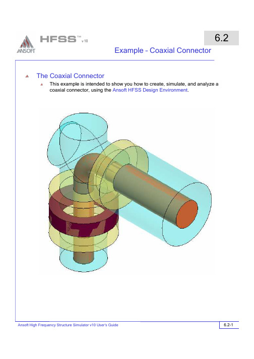
Example –Coaxial Connector 6.2-1The Coaxial ConnectorThis example is intended to show you how to create, simulate, and analyze a coaxial connector, using the Ansoft HFSS Design Environment .Example –Coaxial Connector6.2-2Ansoft HFSS Design EnvironmentThe following features of the Ansoft HFSS Design Environment are used to create this passive device model3D Solid ModelingPrimitives: Cylinders, Polylines, CirclesCylinders, Polylines, Circles Boolean Operations: Unite, Subtract, and Sweep Unite, Subtract, and SweepBoundaries/ExcitationsPorts:Wave Ports and Terminal Lines Analysis Sweep: Fast Frequency: Fast Frequency ResultsCartesian plottingField Overlays:3D Field Plots, Animations, Cut 3D Field Plots, Animations, Cut--PlanesExample –Coaxial Connector6.2-3Getting StartedLaunching Ansoft HFSS1.To access Ansoft HFSS, click the Microsoft Start Start button, select Programs ProgramsPrograms, and select the Ansoft, HFSS 10Ansoft, HFSS 10program group. Click HFSS 10HFSS 10HFSS 10.Setting Tool OptionsTo set the tool options:Note:Note: In order to follow the steps outlined in this example, verify that the following tool options are set :1.Select the menu item Tools > Options > HFSS Options2.HFSS Options Window:1.Click the General General tabUse Wizards for data entry when creating new boundaries: :CheckedDuplicate boundaries with geometry: : Checked2.Click the OK OK button3.Select the menu item Tools > Options > 3D Modeler Options Tools > Options > 3D Modeler Options.4.3D Modeler Options Window:1.Click the Operation Operation tabAutomatically cover closed polylines: :Checked 2.Click the Drawing Drawing tabEdit property of new primitives: : Checked3.Click the OK OK buttonExample –Coaxial Connector6.2-4 Opening a New ProjectTo open a new project:1.In an Ansoft HFSS window, click the On the Standard toolbar, or selectthe menu item File > New.2.From the Project menu, select Insert HFSS Design.Set Solution TypeTo set the solution type:1.Select the menu item HFSS > Solution Type2.Solution Type Window:1.Choose Driven TerminalDriven Terminal2.Click the OKOK buttonExample –Coaxial Connector6.2-5Creating the 3D ModelSet Model UnitsTo set the units:1.Select the menu item 3D Modeler > Units2.Set Model Units:1.Select Units: cm cm2.Click the OK OK buttonSet Default MaterialTo set the default material:ing the 3D Modeler Materials toolbar, choose Select Select2.Select Definition Window:1.Type pec pec in the Search by Name Search by Name field2.Click the OK OK buttonExample –Coaxial Connector6.2-6Create the Conductor 1To create the conductor1.Select the menu item Draw > Cylindering the coordinate entry fields, enter the cylinder positionX: 0.00.00.0, Y: 0.00.00.0, Z: 0.00.00.0, Press the Enter Enter key ing the coordinate entry fields, enter the radius:dX: 0.1520.1520.152, dY: 0.00.00.0, dZ: 0.00.00.0, Press the Enter Enter key 4.Using the coordinate entry fields, enter the height:dX: 0.00.00.0, dY: 0.00.00.0, dZ: 1.4481.4481.448, Press the Enter Enter key To set the name:1.Select the Attribute Attribute tab from the Properties Properties window.2.For the Value Value of Name Name type: Conductor1Conductor13.Click the OK OK buttonTo fit the view:1.Select the menu item View > Fit All > Active View . Or press the CTRL+D CTRL+D keyCreate Offset Coordinate SystemTo create an offset Coordinate System:1.Select the menu item 3D Modeler > Coordinate System > Create > Relative CS > Offseting the coordinate entry fields, enter the originX: 0.00.00.0, Y: 0.00.00.0, Z: 1.448, 1.448,1.448, Press the Enter Enter key Create a SectionTo section the conductor1.Select the menu item Edit > Select All Visible . . Or press the CTRL+A CTRL+A key.2.Select the menu item 3D Modeler > Surface > Section3.Section WindowSection Plane:XYClick the OK OKOK buttonExample –Coaxial Connector6.2-7Rename the SectionTo set the name:1.Select the menu item HFSS > List2.From the Model Model tab, select the object named Section1Section13.Click the Properties PropertiesProperties button 1.For the Value Value of Name Name type: Bend Bend 2.Click the OK OK button 4.Click the DoneDone buttonSet Grid PlaneTo set the grid plane:1.Select the menu item 3D Modeler > Grid Plane > YZ Create Conductor BendTo create the bend:1.Select the menu item Draw > Arc > Center Point ing the coordinate entry fields, enter the vertex point:X: 0.00.00.0, Y: 0.40.40.4, Z: 0.00.00.0, Press the Enter Enter key ing the coordinate entry fields, enter the radial point:X: 0.00.00.0, Y: 0.00.00.0, Z: 0.00.00.0, Press the EnterEnter key ing the coordinate entry fields, enter the sweep arc length:X: 0.00.00.0, Y: 0.40.40.4, Z: 0.40.40.4,Press the Enter Enter key ing the mouse, right-click and select DoneDone 6.Click the OK OK button when the Properties dialog appears Sweep Bend:1.Select the menu item Edit > Select > By Name2.Select Object Dialog,1.Select the objects named: Bend, Polyline1Bend, Polyline12.Click the OK OKOK button 3.Select the menu item Draw > Sweep > Along Path 4.Sweep along path WindowAngle of twist:0Draft Angle: 00Draft Type: Round RoundClick the OK OKOK buttonExample –Coaxial Connector6.2-8Set Grid PlaneTo set the grid plane:1.Select the menu item 3D Modeler > Grid Plane > XZ Create Offset Coordinate SystemTo create an offset Coordinate System:1.Select the menu item 3D Modeler > Coordinate System > Create > Relative CS > Offseting the coordinate entry fields, enter the originX: 0.00.00.0, Y: 0.40.40.4, Z: 0.4,0.4, 0.4, Press the EnterEnter key Create the Conductor 2To create the conductor1.Select the menu item Draw > Cylinder ing the coordinate entry fields, enter the cylinder positionX: 0.00.00.0, Y: 0.00.00.0, Z: 0.00.00.0,Press the EnterEnter key ing the coordinate entry fields, enter the radius:dX: 0.1520.1520.152, dY: 0.00.00.0, dZ: 0.00.00.0,Press the Enter Enter key ing the coordinate entry fields, enter the height:dX: 0.00.00.0, dY: 0.4360.4360.436, dZ: 0.00.00.0,Press the EnterEnter key To set the name:1.Select the Attribute Attribute tab from the Properties Properties window.2.For the Value Value of Name Name type: Conductor2Conductor23.Click the OK OK buttonTo fit the view:1.Select the menu item View > Fit All > Active View. Create Offset Coordinate SystemTo create an offset Coordinate System:1.Select the menu item 3D Modeler > Coordinate System > Create > Relative CS > Offseting the coordinate entry fields, enter the originX: 0.00.00.0, Y: 0.4360.4360.436, Z: 0.00.00.0, Press the Enter Enter keyExample –Coaxial Connector6.2-9 Create the Conductor 3To create the conductor1.Select the menu item Draw > Cylindering the coordinate entry fields, enter the cylinder positionX: 0.00.00.0, Y: 0.00.00.0, Z: 0.00.00.0,Press the EnterEnter keying the coordinate entry fields, enter the radius:dX: 0.2250.2250.225, dY: 0.00.00.0, dZ: 0.00.00.0, Press the EnterEnter keying the coordinate entry fields, enter the height:dX: 0.00.00.0, dY: 1.31.31.3, dZ: 0.00.00.0, Press the EnterEnter keyTo set the name:1.Select the AttributeAttribute tab from the PropertiesProperties window.2.For the ValueValue of NameName type: Conductor3Conductor33.Click the OKOK buttonTo fit the view:1.Select the menu item View > Fit All > Active View.Group the ConductorsTo group the conductors:1.Select the menu item Edit > Select All Visible. . Or press the CTRL+ACTRL+A key.2.Select the menu item, 3D Modeler > Boolean > UniteTo fit the view:1.Select the menu item View > Fit All > Active View.Set Default MaterialTo set the default material:ing the 3D Modeler Materials toolbar, choose vacuumvacuumExample –Coaxial Connector6.2-10Create the Female EndTo create the female end:1.Select the menu item Draw > Cylinder ing the coordinate entry fields, enter the cylinder positionX: 0.00.00.0, Y: 0.00.00.0, Z: 0.00.00.0, Press the EnterEnter key ing the coordinate entry fields, enter the radius:dX: 0.5110.5110.511, dY: 0.00.00.0, dZ: 0.00.00.0, Press the Enter Enter key ing the coordinate entry fields, enter the height:dX: 0.00.00.0, dY: 1.31.31.3, dZ: 0.00.00.0, Press the Enter Enter key To set the name:1.Select the Attribute Attribute tab from the Properties Properties window.2.For the Value Value of Name Name type: Female Female3.Click the OK OK buttonTo fit the view:1.Select the menu itemView > Fit All > Active View . Create the Female BendTo create the bend:1.Select the menu itemDraw > Cylinder ing the coordinate entry fields, enter the cylinder positionX: 0.0, Y: 0.0, Z: 0.0,X: 0.0, Y: 0.0, Z: 0.0, Press the Enter key ing the coordinate entry fields, enter the radius:dX dX: 0.351, : 0.351, : 0.351, dY dY dY: 0.0, : 0.0, : 0.0, dZ dZ dZ: 0.0, : 0.0,: 0.0, Press the Enter key ing the coordinate entry fields, enter the height:dX dX: 0.0, : 0.0, : 0.0, dY dY dY: : : --1.236, 1.236, dZdZ dZ: 0.0, : 0.0,: 0.0, Press the Enter key To set the name:1.Select the Attribute Attribute tab from the Properties Properties window.2.For the Value Value of Name Name type: FemaleBendFemaleBend 3.Click the OK OK buttonTo fit the view:1.Select the menu item View > Fit All > Active View .Example –Coaxial Connector6.2-11Set Working Coordinate SystemTo set the working coordinate system:1.Select the menu item 3D Modeler > Coordinate System > Set Working CS2.Select Coordinate System Window,1.From the list, select the CS: GlobalGlobal 2.Click the Select SelectbuttonSet Grid PlaneTo set the grid plane:1.Select the menu item 3D Modeler > Grid Plane > XYCreate the Male EndTo create the male end:1.Select the menu itemDraw > Cylindering the coordinate entry fields, enter the cylinder positionX: 0.0, Y: 0.0, Z: 0.0,X: 0.0, Y: 0.0, Z: 0.0, Press the Enter key ing the coordinate entry fields, enter the radius:dX dX: 0.351, : 0.351, : 0.351, dY dY dY: 0.0, : 0.0, : 0.0, dZ dZ dZ: 0.0, : 0.0,: 0.0, Press the Enter key ing the coordinate entry fields, enter the height:dX dX: 0.0, : 0.0, : 0.0, dY dY dY: 0.0, : 0.0, : 0.0, dZdZ dZ: 2.348, : 2.348,: 2.348, Press the Enter key To set the name:1.Select the Attribute Attribute tab from the Properties Properties window.2.For the Value Value of Name Name type: Male Male3.Click the OK OK buttonTo fit the view:1.Select the menu item View > Fit All > Active View .Example –Coaxial Connector6.2-12Group the Vacuum ObjectsTo unite the objects Female, To unite the objects Female, FemaleBend FemaleBend and Male:1.Select the menu item Edit > Select > By Name2.Select Object Dialog,1.Select the objects named: Female, Female, Female, FemaleBend FemaleBend FemaleBend, Male , Male2.Click the OK OKOK button 3.Select the menu item, 3D Modeler > Boolean > UniteTo fit the view:1.Select the menu item View > Fit All > Active View .Add New MaterialTo add a new material:ing the 3D Modeler Materials toolbar, choose Select Select2.From the Select Definition window, click the Add Material Add Material button3.View/Edit Material Window:1.For the Material Name Material Name type: My_Ring My_Ring2.For the Value Value of Relative Permittivity Relative Permittivity type: 333.Click the OK OK button4.Click the OK OK buttonExample –Coaxial Connector6.2-13Create the RingTo create the ring:1.Select the menu itemDraw > Cylindering the coordinate entry fields, enter the cylinder positionX: 0.00.00.0, Y: 0.00.00.0, Z: 0.7360.7360.736, Press the Enter Enter key ing the coordinate entry fields, enter the radius:dX: 0.5110.5110.511, dY: 0.00.00.0, dZ: 0.00.00.0, Press the Enter Enter key ing the coordinate entry fields, enter the height:dX: 0.00.00.0, dY: 0.00.00.0, dZ: 0.2360.2360.236, Press the Enter Enter key To set the name:1.Select the Attribute Attribute tab from the Properties Properties window.2.For the Value Value of Name Name type: RingRing 3.Click the OK OK buttonTo fit the view:1.Select the menu itemView > Fit All > Active View .Complete the RingTo select the objects Ring and Male:1.Select the menu item Edit > Select > By Name2.Select Object Dialog,1.Select the objects named: Ring, Female Ring, Female2.Click the OK OKOK button To complete the ring:1.Select the menu item 3D Modeler > Boolean > Subtract2.Subtract WindowBlank Parts: Ring RingTool Parts: FemaleFemale Clone tool objects before subtract: CheckedClick the OK OK buttonExample –Coaxial Connector6.2-14Add New MaterialTo add a new material:ing the 3D Modeler Materials toolbar, choose Select Select2.From the Select Definition window, click the Add Material Add Material button3.View/Edit Material Window:1.For the Material Name Material Name type: My_Teflon My_Teflon2.For the Value Value of Relative Permittivity Relative Permittivity type: 2.12.13.Click the OK OKbutton 4.Click the OK OKbuttonCreate the Male TeflonTo create the To create the teflon teflon teflon::1.Select the menu item Draw > Cylindering the coordinate entry fields, enter the cylinder positionX: 0.00.00.0, Y: 0.00.00.0, Z: 0.460.460.46, Press the Enter Enter key ing the coordinate entry fields, enter the radius:dX: 0.5110.5110.511, dY: 0.00.00.0, dZ: 0.00.00.0, Press the Enter Enter key ing the coordinate entry fields, enter the height:dX: 0.00.00.0, dY: 0.00.00.0, dZ: 0.7880.7880.788, Press the Enter Enter key To set the name:1.Select the Attribute Attribute tab from the Properties Properties window.2.For the Value Value of Name Name type: MaleTeflonMaleTeflon 3.Click the OK OK buttonTo fit the view:1.Select the menu item View > Fit All > Active View.Example –Coaxial Connector6.2-15Create Wave Port Excitation 1Note:Note: To simplify the instructions, a 2D object will be created to represent the port. This is not a requirement for defining ports. Graphical face selection can be used as an alternative.To create a circle that represents the port:1.Select the menu itemDraw > Circleing the coordinate entry fields, enter the center positionX: 0.00.00.0, Y: 0.00.00.0, Z: 0.00.00.0, Press the EnterEnter key ing the coordinate entry fields, enter the radius of the circle:dX: 0.3510.3510.351, dY: 0.00.00.0, dZ: 0.00.00.0, Press the Enter Enter key To set the name:1.Select the Attribute Attribute tab from the Properties Properties window.2.For the Value Value of Name Name type: p1p13.Click the OK OK buttonTo select the object p1:1.Select the menu item Edit > Select > By Name2.Select Object Dialog,1.Select the objects named: p1p12.Click the OK OKOK button NoteNote: You can also select the object from the Model TreeExample –Coaxial Connector6.2-16Create Wave Port Excitation 1 (Continued)To assign wave port excitation1.Select the menu item HFSS > Excitations > Assign > Wave Port2.Wave Port : General: p1p1p1, 2.Click the Next Next button3.Wave Port : Terminals1.Number of Terminals: 11,2.For T1T1T1, click the Undefined Undefinedcolumn and select New Line New Line ing the coordinate entry fields, enter the vector positionX: 0.3510.3510.351, Y: 0.00.00.0, Z: 0.00.00.0, Press the EnterEnter key ing the coordinate entry fields, enter the vertexdX: --0.1990.199, dY: 0.00.00.0, dZ: 0.00.00.0, Press the Enter Enter key 5.Click the Next Next button4.Wave Port : Differential Pairs1.Click the Next Next button5.Wave Port : Post Processing1.Full Port Impedance: 50506.Click the Finish FinishbuttonSet Working Coordinate SystemTo set the working coordinate system:1.Select the menu item 3D Modeler > Coordinate System > Set Working CS2.Select Coordinate System Window,1.From the list, select the CS: RelativeCS3RelativeCS32.Click the Select SelectbuttonSet Grid PlaneTo set the grid plane:1.Select the menu item 3D Modeler > Grid Plane > XZExample –Coaxial Connector6.2-17Create Wave Port Excitation 2Note:Note: To simplify the instructions, a 2D object will be created to represent the port. This is not a requirement for defining ports. Graphical face selection can be used as an alternative.To create a circle that represents the port:1.Select the menu item Draw > Circleing the coordinate entry fields, enter the center positionX: 0.00.00.0, Y: 1.31.31.3, Z: 0.00.00.0, Press the Enter Enter key ing the coordinate entry fields, enter the radius of the circle:dX: 0.5110.5110.511, dY: 0.00.00.0, dZ: 0.00.00.0, Press the Enter Enter key To set the name:1.Select the Attribute Attribute tab from the Properties Properties window.2.For the Value Value of Name Name type: p2p23.Click the OK OK buttonTo select the object p2:1.Select Object Dialog,1.Select the objects named: p2p22.Click the OK OKOK buttonExample –Coaxial Connector6.2-18Create Wave Port Excitation 2 (Continued)To assign wave port excitation1.Select the menu item HFSS > Excitations > Assign > Wave Port2.Wave Port : General: p2p2p2, 2.Click the Next Next button3.Wave Port : Terminals1.Number of Terminals: 11,2.For T1T1T1, click the Undefined Undefinedcolumn and select New Line New Line ing the coordinate entry fields, enter the vector positionX: 0.5110.5110.511, Y: 1.31.31.3, Z: 0.00.00.0, Press the EnterEnter key ing the coordinate entry fields, enter the vertexdX: --0.2860.286, dY: 0.00.00.0, dZ: 0.00.00.0, Press the Enter Enter key 5.Click the Next Next button4.Wave Port : Differential Pairs1.Click the Next Next button5.Wave Port : Post Processing1.Full Port Impedance : 50502.Click the Finish Finish buttonExample –Coaxial Connector6.2-19Create the Female TeflonTo create the Teflon:1.Select the menu item Draw > Cylinder2.Using the coordinate entry fields, enter the cylinder position X: 0.0, Y: 0.0, Z: 0.0,X: 0.0, Y: 0.0, Z: 0.0, Press the Enter key ing the coordinate entry fields, enter the radius:dX dX: 0.511, : 0.511, : 0.511, dY dY dY: 0.0, : 0.0, : 0.0, dZ dZ dZ: 0.0, : 0.0,: 0.0, Press the Enter key ing the coordinate entry fields, enter the height:dX dX: 0.0, : 0.0, : 0.0, dY dY dY: : : --0.236, 0.236, dZdZ dZ: 0.0, : 0.0,: 0.0, Press the Enter key To set the name:1.Select the Attribute Attribute tab from the Properties Properties window.2.For the Value Value of Name Name type: FemaleTeflonFemaleTeflon 3.Click the OK OK buttonTo fit the view:1.Select the menu item View > Fit All > Active View.Complete the Vacuum ObjectTo select the objects Female, To select the objects Female, MaleTeflon MaleTeflon MaleTeflon, , , FemaleTeflon FemaleTeflon1.Select the menu item Edit > Select > By Name2.Select Object Dialog,1.Select the objects named: Female, Female, Female, MaleTeflon MaleTeflon MaleTeflon, , , FemaleTeflon FemaleTeflon2.Click the OK OKOK button To complete the To complete the vacumm vacumm objects:1.Select the menu item 3D Modeler > Boolean > Subtract 2.Subtract WindowBlank Parts: Female FemaleTool Parts: MaleTeflon MaleTeflon MaleTeflon,, , FemaleTeflon FemaleTeflonClone tool objects before subtract: CheckedClick the OK OK buttonExample –Coaxial Connector6.2-20Complete the ModelTo complete the model:1.Select the menu item Edit > Select > By Name2.Select Object Dialog,1.Select the objects named: Conductor1, Female, Conductor1, Female, Conductor1, Female, MaleTeflon MaleTeflon MaleTeflon, , FemaleTeflon2.Click the OK OKOK button 3.Select the menu item 3D Modeler > Boolean > Subtract 4.Subtract WindowBlank Parts: Female, Female, Female, FemaleTeflon FemaleTeflon FemaleTeflon, , , MaleTeflon MaleTeflonTool Parts: Conductor1Conductor1Clone tool objects before subtract: CheckedClick the OK OK buttonBoundary DisplayTo verify the boundary setup:1.Select the menu item HFSS > Boundary Display (Solver View)2.From the Solver View of Boundaries, toggle the Visibility check box for the boundaries you wish to display.Note:The background (Perfect Conductor) is displayed as the outer outer boundary.Note:The Perfect Conductors are displayed as the smetal smetal boundary.Note:Select the menu item, View > Visibility to hide all of the geometry objects. This makes it easier to see the boundary 3.Click the Close Close button when you are finishedExample –Coaxial Connector6.2-21Analysis SetupCreating an Analysis SetupTo create an analysis setup:1.Select the menu item HFSS > Analysis Setup > Add Solution Setup2.Solution Setup Window:1.Click the General General tab::Solution Frequency: 8.1GHz : 8.1GHzMaximum Number of Passes: 1010Maximum Delta S: 0.020.022.Click the OK OK button3.Click the Options Options tab::Minimum Converged Passes: 224.Click the OKOK buttonAdding a Frequency SweepTo add a frequency sweep:1.Select the menu item HFSS > Analysis Setup > Add Sweep1.Select Solution Setup: Setup1 Setup12.Click the OK OK button2.Edit Sweep Window:1.Sweep Type: Fast : Fast2.Frequency Setup Type: Linear Count : Linear CountStart:0.1GHzStop: 8.1GHz : 8.1GHzCount: 801: 801Save Fields: Checked3.Click the OK OK buttonExample –Coaxial Connector6.2-22Save ProjectTo save the project:1.In an Ansoft HFSS window, select the menu item File > Save As .2.From the Save As Save AsSave As window, type the Filename: hfss_coax hfss_coax 3.Click the Save Save buttonAnalyzeModel ValidationTo validate the model:1.Select the menu item HFSS > Validation Check2.Click the Close CloseClose button Note:To view any errors or warning messages, use the MessageManager.AnalyzeTo start the solution process:1.Select the menu item HFSS > AnalyzeExample –Coaxial Connector6.2-23Solution DataTo view the Solution Data:1.Select the menu item HFSS > Results > Solution DataTo view the Profile:1.Click the Profile Profile Tab.To view the Convergence:1.Click the Convergence Convergence TabNote: Note: The default view is for convergence is Table TableTable. Select the Plot Plot radio button to view a graphical representations ofthe convergence data.To view the Matrix Data:1.Click the Matrix Data Matrix Data TabNote:Note: To view a real-time update of the Matrix Data, set the Simulation to Setup1, Last AdaptiveSetup1, Last Adaptive 2.Click the Close Close buttonExample –Coaxial Connector6.2-24Create ReportsCreate Terminal S Create Terminal S--Parameter Plot vs. Adaptive PassNote:Note: If this report is created prior to or during the solution process, a real-time update of the results are displayedTo create a report:1.Select the menu item HFSS > Results > Create Report2.Create Report Window::1.Report Type: Terminal S Parameters Terminal S Parameters2.Display Type: Rectangular Rectangular3.Click the OK OKOK button 3.Traces Window::1.Solution: Setup1: Adaptive1Setup1: Adaptive12.Click the X XX tab e Primary Sweep: : Unchecked2.Category: Variables Variables3.Quantity: Pass : Pass3.Click the Y Y tab1.Category: Terminal S Parameter Terminal S Parameter2.Quantity: St(p1,p1), St(p1,p2), St(p1,p1), St(p1,p2),3.Function: dB dB4.Click the Add Trace Add Trace button4.Click the Done Done buttonExample –Coaxial Connector6.2-25Create Terminal S Create Terminal S--Parameter Plot Parameter Plot --MagnitudeTo create a report:1.Select the menu item HFSS > Results > Create Report2.Create Report Window::1.Report Type: Terminal S Parameters Terminal S Parameters2.Display Type: Rectangular Rectangular3.Click the OK OKOK button 3.Traces Window::1.Solution: Setup1: Sweep1Setup1: Sweep12.Domain: Sweep Sweep3.Click the Y Y tab1.Category:Terminal S Parameter2.Quantity: St(p1,p1), St(p1,p2), St(p1,p1), St(p1,p2),3.Function: dB dB4.Click the Add Trace Add Tracebutton 4.Click the Done Done buttonExample –Coaxial Connector6.2-26Create Terminal S Create Terminal S--Parameter Plot Parameter Plot --PhaseTo create a report:1.Select the menu item HFSS > Results > Create Report2.Create Report Window::1.Report Type: Terminal S Parameters Terminal S Parameters2.Display Type: Rectangular Rectangular3.Click the OK OKOK button 3.Traces Window::1.Solution: Setup1: Sweep1Setup1: Sweep12.Domain: Sweep Sweep3.Click the Y Y tab1.Category:Terminal S Parameter2.Quantity: St(p1,p1), St(p1,p2), St(p1,p1), St(p1,p2),3.Function: ang_deg ang_deg4.Click the Add Trace Add Trace button4.Click the Done Done buttonExample –Coaxial Connector6.2-27 Field OverlaysCreate Field OverlayTo create a field plot:1.Select the Global YZ Planeing the Model Tree, expand PlanesPlanes2.Select Global:YZGlobal:YZ2.Select the menu item HFSS > Fields >HFSS > Fields > FieldsFields> E >> E > Mag_EMag_E3.Create Field Plot Window1.Solution: Setup1 :Setup1 :Setup1 : LastAdaptiveLastAdaptive2.Quantity: Mag_EMag_E3.In Volume: AllAll4.Click the DoneDone buttonTo modify a Magnitude field plot:1.Select the menu item HFSS > Fields > Modify Plot Attributes2.Select Plot Folder Window:1.Select: E FieldE Field2.Click the OKOK button3.E-Field Window:1.Click the ScaleScaleScale tab1.Select Use LimitsUse Limits2.Min:1.03.Max:1000.04.Scale: LogLog2.Click the CloseClose buttonExample –Coaxial Connector6.2-28Edit SourcesTo Modify a Terminal excitation:1.Select the menu item HFSS > Fields > Edit Sources 2.Select p2:T1p2:T1from the Edit Sources windowCheck the Terminated Terminated box3.Click the OK OK buttonTo Select the Electric Field plot:1.Expand the Project tree2.Expand the Field Overlays Field Overlays3.Click on the E Field E Field or Mag_E1Mag_E1to display the field plotField AnimationsTo Animate a Magnitude field plot:1.Select the menu item View > Animate 2.In the Swept Variable Swept Variable tab, accept defaults settings:1.Swept variable: Phase Phase2.Start: 0deg 0deg3.Stop: 180deg 180deg4.Steps: 993.Click the Close Close button。

HFSS的入门操作

•
第二个点的相对坐标（140,160,80）
• 空气盒子的尺寸要求是保证空气的辐射边界离天线的距离超过四分之一工作波长，空气盒子太小则仿真结果不准确，太大需要更多的仿真时间。
• 选中刚画的空气盒子box2，在properties窗口的material属性edit-》选中air材料。 • 选中刚画的空气盒子box2，右键菜单-》AssignBoundary-》Radiation-》确定
按上面的信息填写以及选择，按ok
执行仿真，（仿真结束后）生成结果
HFSS-》results-》Creat modal Solution data Report-》Rectangular plot
默认生成S11
dB(S(1,1))
0.00 -1.25
-3.25
-5.25 -7.25
-9.25
-11.25 2.00
设置激励（相当于接上接头）
• 绘制一个连接正面微带线以及背面接地板的矩形。
•Hale Waihona Puke 首先将绘制坐标系选为zx，然后按下图绘制一个小矩形等效馈电接口
• Draw Rectangle: 第一个点（28.5,0,0）
•
第二个点（3,0，-1.6）
• 选中该矩形rectangle5，
• 右键菜单-》Assign excitation-》lump port-》默认输入阻抗50欧姆下一步-》点击integration line的 none，选new line，此时进入绘图界面画积分线，第一个点选端口矩形rectangle5与接地板相连的边的中点，即（30,0，-1.6）第二个点选端口矩形rectangle5与微带线相连的边的中点，相对坐标为（0,0,1.6）。

HFSS教程第3章AnsoftHFSS使用介绍

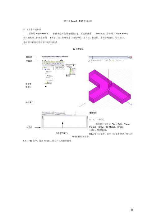
第三章Ansoft HFSS 使用介绍3. 1工作环境介绍要应用Ansoft HFSS软件来分析高频电磁场问题，首先要熟悉HFSS 的工作环境。

Ansoft HFSS软件的典型工作环境如图 1所示。

该工作环境窗口由菜单栏、工具栏、状态栏、工程管理窗口、特性窗口、进度窗口和信息管理窗口几部分组成。

3D 模型窗口进度窗口3. 1 . 1菜单栏菜单栏中包含了 File 、Edit 、View 、Project 、Draw 、3D Model 、HFSS 、Tools 、Windows 、Help 等下拉菜单，这些下拉菜单包含了所有的HFSS 操作和命令。

1.1.1 File 菜单：管理HFSS 工程文件以及打印操作。

菜单栏——_ 工具栏 ______工程管理窗口特性窗口ZaU E-L*- Ki-^- tri-j*ci ■■ 耳心址* T□ •打 ^ £ • >曲•鼻«hU-W P 曰卜T*r* ■ 1)4 4]HI iF审 l|!> MM*ri«life IHF^-L*i^. h A Sto dba ft S * * * ft< 9 n M iJ * bt0 it .0 rs > ari £]!*刖■lhai+ i*?idjEn>H-L状态栏信息管理窗口□世郎 Ctrl+HOpsn, . . Ctrl+0Close H SaveCtrl+5Save As.』_A E Tecbnoloigy FilePrint PreviewS Erird …. Ctrl+T1 E AKFSSpjt\Froject5. hfn2 E ： VWSSpj tVPatchkrray.3 K:\HFSSpj t\Fraj»t4. hfEE4 EAKFSSpjt\Projec-t3. h£*至 E:\HfSSpjt\Frojtct2. hf 宝& E 2 MffSSpj iVpatclL hfs sI E:\HFSSpjt\PIF^. hfss 3 I:Vsj^. hfn K M I t1.1.2 Edit 菜单：修正3D 模型及撤销和恢复等操作。

3 3207-100兆天线用户手册

3207型号天线系统设置和用户手册The World Leader inSubsurface Imaging™美国劳雷工业有限公司目录3207型天线 (3)3207P和3207AP操作注意事项 (4)1.理解电子单元 (4)2.操作模式 (6)2.1双体天线浅部探测模式 (6)2.2双体天线深部探测模式 (7)2.3单体天线（3207AP） (8)3仪器部件和连接装置图 (10)3.1部件列表 (10)3.2硬件连接图 (11)4距离测量选项 (12)5软件系统设置--标准设置 (14)5.1 3207AP单体天线参数设置 (14)5.2 3207P双体天线参数设置 (15)5.3 天线参数 (15)附图3207型天线3207型号天线用于深部探测，可有效对地下土壤和岩石结构成图。

3207型天线有2种组成方式。

单体方式：有单个天线3207盒子构成，包括一个769DA2发射/接收电子单元，即每个电子单元电路板上设置了发射和接收切换开关。

鉴于该天线仅仅有一个3207盒子，需要进行深部探测而场地范围又小的情况下，单体天线是一个理想选择。

这种形式天线定义为3207AP。

3207天线对，用于深部探测、共中心点CMP分析。

包括两个3207盒子，中间通过玻璃纤维竿子连接，或者采用不通的间距用于CMP 测量分析。

一个盒子用于发射天线，另外一个盒子用于接收天线。

接收天线采用769DA2型号电子单元，仅仅用于接收电磁波，通过out 输出端口连接至发射天线电子单元。

发射天线采用778型号高功率发射电子单元，通过一个电缆连接至769DA2。

无论记录长度大小，都可以使用3207天线对测量。

这种天线形式定义为3207P。

注意：570型号光缆发射连接器用于3207P天线对。

570型号光缆发射器用于取代同轴电缆。

利用570型号部件可以取得更好的探测效果。

建议单独购买570型号光缆。

3207型号天线中心频率为100MHz。

GSSI公司强烈建议在使用SIR-3000和100兆天线对时使用570型号光缆发射器。

hfss中文教程手册下载

创建项目目录
在使用 Ansoft HFSS 求解时，第一步就是要创建一个目录和项目，用于存储与问题相关的数据。一个项目目录包括用 Ansoft 软件来创建的某一系列的项目。你可以使用项目目录对项目进行任意分类。例如，你也许想在一个项目目录下存储与某一特定用途有关的所有项目，那么，你可以在缺省目录下建立一个项目目录。 Project manager 应该仍然在屏幕上显示，你可以为使用 getting started 向导为你创建的项目加 getstart 目录。注意：如果你已经通过另一 getting started 指南创建了项目目录，直接跳到“Creat a Project”这一步。 Ø 为这个例子加一个项目目录： 1．在窗口左上方的 Project Directory 中选择 Add。就会出现下图所示的窗
添加新项目
Ø 添加新项目： 1. 在菜单左上部的 Projects 块中选择 New。将出现如下图所示的窗口。
2. 在 Name 里输入 eigen。使用 Back Space 和 Delete 键来修改输入。 3. 选择创建项目的类型，单击列于 Type 中的软件包。会出现一个列有所
有可选 Ansoft 软件包的菜单。选中 Ansoft High Frequency Structure Simulator 7 作为项目类型。 4. 可选项，在 Created By 中输入你的名字。注意：如果你在工作站和使用 Microsoft Windows NT 的 PC 上运行软件的话，人名会以缺省的方式自动出现在系统中。 5．取消选定 Open project upon creation。当选定这项时，单击 OK 就会打开项目。但现在还不要打开项目。 6. 选择 OK 创建项目。刚刚输入的信息现在将在 Selected Project 块的相应地方显示出来。选中 Writable，表明你已经访问过这个项目。

采用电磁仿真软件HFSS数值仿真同轴连接器及其电磁场性能

课程设计报告设计题目：采用电磁仿真软件HFSS数值仿真同轴连接器及其电磁场性能分析学院：电子工程学院专业：电子信息工程班级： 0212XX学号： 0212XXXX姓名： XXX电子邮件：日期： 2016年01月成绩：指导教师：李 X西安电子科技大学电子工程学院课程设计任务书学生姓名指导教师职称学生学号 0212 专业电子信息工程题目采用电磁仿真软件HFSS 数值仿真同轴连接器及其电磁场性能分析任务与要求根据《电磁场与电磁波》和《微波技术基础》课程的理论学习，通过学习电磁仿真软件Ansys HFSS ，掌握其基本原理和使用方法，并采用HFSS 数值仿真——同轴连接器，分析其输入阻抗特性、网络参数特性、同轴线内部场分布和电流分布等传输线参数，以巩固所学习的电磁场传输问题。

要求：（1）学习Ansys HFSS 全波电磁仿真软件；（2）掌握HFSS 的使用方法，并能准确地进行数值仿真计算；（3）全波仿真同轴连接器，给出全波仿真同轴连接器的网络散射参数随频率的变化特性，同轴连接器中的电磁场分布图以及各端口的场特性。

开始日期 2016年 01月 06 日完成日期 2016年 01月20 日课程设计所在单位电子工程学院本表格由电子工程学院网络信息中心编辑录入 .…………………………装………………………………订………………………………线………………………………………………………………采用HFSS数值仿真同轴连接器及其电磁场性能分析XXX（西安电子科技大学电子工程学院，陕西西安 710071）摘要：本文首先简要介绍了同轴线及同轴连接器的概念，并利用HFSS电磁仿真软件对同轴弯头连接器进行了仿真，给出了同轴连接器的网络散射参数随频率的变化特性，同轴连接器中的电磁场分布图以及各端口的电磁场特性。

通过HFSS仿真软件将抽象的电磁场概念具体化，有助于对微波课程的进一步理解。

射频同轴连接器设计理论基础

射频传输线、连接元件和过渡元件简述第一节射频传输线射频同轴连接器的设计一、同轴传输线的特性阻抗1 同轴传输线的特性阻抗的一般公式射频同轴连接器由一段同轴传输线、连接机构绝缘支架组成。

所以，对同轴传输线的特性阻抗有一个比较全面的了解对射频同轴连接器的设计是非常重要的。

同轴传输线特性阻抗的一般公式：Cj G L j R Z ωω++='0 （1）上式中： Z o1—特性阻抗，欧姆R —每单位长度上导体的内部电阻，欧姆/米G —每单位长度上介质的电导，西门子/米L —每单位长度的电感，享/米C —每单位长度的电容，法/米ω=2πff —频率，赫当R=G=0时，公式（1）简化为：CL Z =0 (2) 在微波频率，导体的内部电感是很小的，每单位长度上的电感很接近于每单位长度上的外部电感：d D L ln 21πμ=（3）上式中：L —每单位长度的外部电感，享/米 μ?=μr μo — 介质的导磁率, 享/米 μr —介质的相对导磁率μo =4π×10-7—真空导磁率，享/米 D —外导体的内径 d —内导体的外径单位长度的电容可按下计算：dD C /ln 21πε=（4）上式中：C — 每单位长度电容，法/米ε1 =εr ε0—介质的介电常数，法/米 εr —— 介质的相对介电常数ε0 =1/C o 2μo —真空介电常数，法/米 C O —在真空中的光速 C O =（±）×108，米/秒将公式（3）和（4）代入（2），并只考虑非磁性介质的情况（μr =）,可得到：dDZ rln00006.095860.590ε±=(5) 请注意,真空光速:001με=C真空导磁率μo 被任意地规定为严格等于4π×10-7享/米。

根据精确地进行的实验我们知道光速为0±300米/秒，因此，εo 并不严格等于1/36π×10-9，根据公式计算，εo 应为1/π×10-9。

HFSS软件使用基础介绍课件(1)

2020/1/10
19
几何变换【Edit】【Arrange】/【Duplicate】平移Move：沿指定矢量线移动至新位置；旋转Rotate：沿指定坐标轴转动；镜像移动Mirror：移动物体至指定平面的镜像位置；沿线复制Along line：沿指定矢量线复制模型；绕轴复制Along Axis：沿指定坐标轴复制模型；镜像复制：沿指定镜面复制模型；
2020/1/10
23
（3）分配边界条件天线处在空气中，新建一个空气块包围住天线，作为求解电磁场的空间，在空气块表面设置“辐射边界条件”，模拟开放的自由空间，常用于天线分析。注：为保证计算准确度，辐射边界距离辐射体不小于1/4工作波长。
2020/1/10
24
2020/1/10
25
选中空气块：【HFSS】【Boundaries】【Assign】【Radiation】 Name项自己命名或者直接采用默认。
47
2020/1/10
48
2.2 HFSS使用介绍
2020/1/10
15
3.举例说明---通道机磁场分布
2020/1/10
16
1.启动软件，新建设计工程；注：“另存为”路径名不要带汉字
2020/1/10
17
2.选择求解类型；【HFSS】【Solution Type】 Driven ModalDriven Modal模式驱动求解类型：计算无源、高频结构的S参数时可选此项，如微带、波导、传输线结构；Driven Terminal终端驱动求解类型：计算多导体传输线端口的S参数，由终端电压和电流描述S矩阵；Eigemode本征模求解类型：主要用于谐振问题的设计，计算谐振结构的频率和场分布、谐振腔体的无载Q值。

1、下载文档前请自行甄别文档内容的完整性，平台不提供额外的编辑、内容补充、找答案等附加服务。
2、"仅部分预览"的文档,不可在线预览部分如存在完整性等问题,可反馈申请退款(可完整预览的文档不适用该条件!)。
3、如文档侵犯您的权益，请联系客服反馈,我们会尽快为您处理(人工客服工作时间：9:00-18:30)。

rf 微波|射频|仿真|通信|电子|EMC|天线|雷达|数值 ---- 专业微波工程师社区: HFSS FULL BOOK v10中文翻译版568页(原801页)(分节水印免费发布版)微波仿真论坛 --组织翻译有史以来最全最强的 HFSS 中文教程感谢所有参与翻译,校对,整理的会员版权申明: 此翻译稿版权为微波仿真论坛()所有. 分节版可以转载. 严禁转载568页完整版.推荐: EDA问题集合(收藏版) 之HFSS问题收藏集合 /hfss.htmlQ: 分节版内容有删减吗? A:没有,只是把完整版分开按章节发布,免费下载.带水印但不影响基本阅读.Q: 完整版有什么优势? A:完整版会不断更新,修正,并加上心得注解.无水印.阅读更方便.Q: 本书结构? A: 前200页为使用介绍.接下来为实例(天线,器件,EMC,SI等).最后100页为基础综述Q: 完整版在哪里下载? A: 微波仿真论坛( /read.php?tid=5454 )Q: 有纸质版吗? A:有.与完整版一样,喜欢纸质版的请联系站长邮寄rfeda@ 无特别需求请用电子版Q: 还有其它翻译吗?A:有专门协助团队之翻译小组.除HFSS外,还组织了ADS,FEKO的翻译.还有正在筹划中的任务! Q: 翻译工程量有多大?A:论坛40位热心会员,120天初译,60天校对.30天整理成稿.感谢他们的付出!Q: 只讨论仿真吗?A:以仿真为主.微波综合社区. 论坛正在高速发展.涉及面会越来越广! 现涉及微波|射频|仿真|通信|电子|EMC|天线|雷达|数值|高校|求职|招聘Q: 特色?A: 以技术交流为主,注重贴子质量,严禁灌水; 资料注重原创; 各个版块有专门协助团队快速解决会员问题; --- 等待你的加入RF rf---射频(Radio Frequency)微波|射频|仿真|通信|电子|EMC|天线|雷达|数值 ---- 专业微波工程师社区: http://bbs.eda .cn rfRF EDA .cnrf---射频(Radio Frequency )致谢名单及详细说明/read.php?tid=5454一个论坛繁荣离不开每一位会员的奉献多交流,力所能及帮助他人,少灌水,其实一点也不难打造国内最优秀的微波综合社区还等什么? 加入 RF EDA .CN 微波社区我们一直在努力微波仿真论坛第二节同轴连接器这个例子教你如何在HFSS设计环境下创建、仿真、分析一个同轴连接器。

微波仿真论坛组织翻译第226 页一.Ansoft HFSS 设计环境以下属性将应用到这一无源器件模型的创建中1．三维立体模型基本元件：柱体（Cylinders），折线（Polylines），圆（Circles）布尔（Boolean）操作：合并（Unite），删除（Subtract），扫频（Sweep）2．边界/激励端口：波端口（Wave Ports）和终端积分线（Terminal Lines）3．分析扫描: 快速频域扫描（Fast Frequency）4．结果笛卡尔直角坐标系绘图(Cartesian Plotting)5．场分布图三维场图绘制(3D field Plots)，场分布动画(Animation)，剪切平面(Cut-Planes)微波仿真论坛组织翻译第227 页二.开始一）启动Ansoft HFSS1．点击微软的开始按钮，选择程序，然后选择Ansoft，HFSS10程序组，点击HFSS10，进入Ansoft HFSS。

二）设置工具选项注意：为了按照本例中概述的步骤，应核实以下工具选项已设置：1．选择菜单中的工具（Tools）>选项（Options）>HFSS选项（HFSS Options）2．HFSS选项窗口：1）点击常规（General）标签a．建立新边界时，使用数据登记项的向导（Use Wizards for data entry when creating new boundaries）：勾上。

b．用几何形状复制边界（Duplicate boundaries with geometry）：勾上。

2）点击OK按钮。

3．选择菜单中的工具（Tools）>选项（Options）>3D模型选项（3D Modeler Options）4．3D模型选项（3D Modeler Options）窗口：1）点击操作（Operation）标签自动覆盖闭合的多段线（Automatically cover closed polylines）：勾上。

2）点击画图（Drawing）标签编辑新建原始结构的属性（Edit property of new primitives）：勾上。

3）点击OK按钮三）打开一个新工程1．在窗口，点击标准工具栏中的新建图标，或者选这菜单中文件（File）>新建（New）。

2．从工程（Project）菜单中选择插入HFSS设计（Insert HFSS Design）。

四）设置解决方案类型（Set Solution Type）1．选择菜单中的HFSS>解决方案类型（Solution Type）2．解决方案类型窗口：1）选择终端驱动（Driven Terminal）2）点击OK按钮。

微波仿真论坛组织翻译第228 页三.创建3D模型一) 设置模型单位（Units）1. 选择下拉菜单3D Modeler>Units2. 设置模型单位：1).选中单位：cm2). 点击“OK”按钮二) 设置默认材料（Default Material）1．使用三维建模材料工具条，选择“Select”2．“选择定义（Select Definition）”窗口：1). 在“按名称搜寻（Search by Name）”文本框中键入“pec”2). 点击“OK”按钮微波仿真论坛组织翻译第229 页三) 创建导体柱1 (Conductor1)A.创建导体柱1．选择下拉菜单Draw >Cylinder应用坐标输入框(coordinate entry fields)，输入圆柱体（cylinder）的位置2.1). X: 0.0, Y: 0.0, Z:0.0, 敲“回车(Enter)”键3．应用坐标输入框，输入圆柱体半径1).dX: 0.152, dY: 0.0, dZ: 0.0, 敲“回车(Enter)”键4．应用坐标输入框，输入圆柱体高度1).dX: 0.0, dY: 0.0, dZ: 1.448, 敲“回车(Enter)”键B.设置名称1．在“Properties”窗口，选择“Attribute”选项卡在“Name”项输入：Conductor12.3．点击“OK”按钮C.调整视图(to fit the view)选择下拉菜单View>Fit All>Active View, 或者按“Ctrl + D”键1.四) 创建平移（offset）坐标系统A.创建平移坐标系统1．选择下拉菜单：3D Modeler >Coordinate System>Create>RelativeCS>Offset2．应用坐标输入框，输入新坐标系原点1). X: 0.0, Y: 0.0, Z:1.448, 敲“回车(Enter)”键五) 创建横截面A.选取导体柱横截面1．选择下拉菜单：Edit>Select All Visible, 或按“CTRL+A”键2．选择下拉菜单：3D Modeler> Surface>Section3．“Section”窗口1). 截取平面：XY2). 点击“OK”按钮六) 横截面重命名A.设置名称1．选择下拉菜单：HFSS>List2．在Model选项卡，选中目标，名称为：Section13．点击属性“Properties”按钮微波仿真论坛组织翻译第230 页1). Name 项输入：Bend 2). 点击“OK ”按钮 4．点击“Done ”按钮七) 设定栅格平面(grid plane)1．选择下拉菜单：3D Modeler>Grid Plane>YZ 微波仿真论坛组织翻译第 231 页2．“选择对象（Select Object ）”对话框 eep>Along Path 九) 设定：3D Modeler>Grid Plane>XZ十) 平移坐标系单：3D Modeler >Coordinate System>Create>Relative CS>Offset r )”键 Draw >Cylinder ter )”键 (Enter )”键八) 创建弯导体 A. 创建导体弯头 1．选择下拉菜单：Draw>Arc >Center Point2．使用坐标输入框，输入圆心坐标 1). X: 0.0, Y: 0.4, Z:0.0, 敲“回车(Enter )”键 3．使用坐标输入框，输入顶点坐标 1). X: 0.0, Y: 0.0, Z:0.0, 敲“回车(Enter )”键4．使用坐标输入框，输入角度扫描长度 1). X: 0.0, Y: 0.4, Z:0.4, 敲“回车(Enter )”键5．点击鼠标右键，并选中功能菜单“Done ”项 6．当属性对话框出现时点击“OK ”按钮 B. 扫描（Sweep ）弯头1．选择下拉菜单：Edit>Select >By Name1).选择目标名称：Bend ，Polyline1 2). 点击“OK ” 按钮3．选择下拉菜单：Draw>Sw 4．“沿路径扫描（Sweep along path ）”窗口 1). Angle of twist 项输入：0 2). Draft Angle 项输入：03). Draft Type 项输入：Round 4). 点击“OK ” 按钮栅格平面1．选择下拉菜单 1．选择下拉菜 2．应用坐标输入框，输入新坐标系原点 1). X: 0.0, Y: 0.4, Z:0.4, 敲“回车(Ente 十一) 创建导体2 A. 创建导体柱1．选择下拉菜单2.应用坐标输入框，输入圆柱体位置 1). X: 0.0, Y: 0.0, Z:0.0, 敲“回车(En 3．应用坐标输入框，输入圆柱体半径 1).dX: 0.152, dY: 0.0, dZ: 0.0, 敲“回车 4．应用坐标输入框，输入圆柱体高度微波仿真论坛组织翻译第 232 页车(Enter )”键 B. 设置名称 ties ”窗口，选择“Attribute ”选项卡 C. 调整视图(to fit the view) ll>Active View 拉菜单：3D Modeler >Coordinate Syst 坐标系原点 nter )”键十三) 创建导体3 Draw >Cylinderter )”键(Enter )”键 (Enter )”键B. 设ties ”窗口，选择“Attribute ”选项卡C.w ) ll>Active ViewSelect All Visible ，或者按“CTRL ＋A ”键 B. 调整视图(to fit the view) All>Active View 1).dX: 0.0, dY: 0.436, dZ: 0.0, 敲“回1．在“Proper 2. 在“Name ”项输入：Conductor23．点击“OK ”按钮1. 选择下拉菜单 View>Fit A 十二) 平移坐标系 1．选择下em>Create>Relative CS>Offset2．应用坐标输入框，输入新 1). X: 0.0, Y: 0.436, Z:0.4, 敲“回车(EA. 创建导体柱1．选择下拉菜单2.应用坐标输入框，输入圆柱体位置 1). X: 0.0, Y: 0.0, Z:0.0, 敲“回车(En 3．应用坐标输入框，输入圆柱体半径 1).dX: 0.225, dY: 0.0, dZ: 0.0, 敲“回车 4．应用坐标输入框，输入圆柱体高度1).dX: 0.0, dY:1.3, dZ: 0.0, 敲“回车置名称 1．在“Proper 2. 在“Name ”项输入：Conductor33．点击“OK ”按钮调整视图(to fit the vie 1. 选择下拉菜单 View>Fit A 十四) 组合前述导体部件 A. 组合前述导体部件 1．选择下拉菜单 Edit > 2．选择下拉菜单：3D Modeler>Boolean>Unite1．选择下拉菜单 View>Fit十五) 设置默认材料工具条，选择“vacuum”1．使用三维建模材料微波仿真论坛组织翻译第233 页十六)创建“Female” 接头A.创建Female接头1．选择下拉菜单Draw >Cylinder应用坐标输入框，输入圆柱体位置2.1). X: 0.0, Y: 0.0, Z:0.0, 敲“回车(Enter)”键3．应用坐标输入框，输入圆柱体半径1).dX: 0.511, dY: 0.0, dZ: 0.0, 敲“回车(Enter)”键4．应用坐标输入框，输入圆柱体高度1).dX: 0.0, dY:1.3, dZ: 0.0, 敲“回车(Enter)”键B.设置名称1．在“Properties”窗口，选择“Attribute”选项卡在“Name”项输入：Female2.3．点击“OK”按钮C.调整视图(to fit the view)1. 选择下拉菜单View>Fit All>Active View十七) 创建“Female”弯头A.创建弯头1．选择下拉菜单Draw >Cylinder应用坐标输入框，输入圆柱体位置2.1). X: 0.0, Y: 0.0, Z: 0.0, 敲“回车(Enter)”键3．应用坐标输入框，输入圆柱体半径1).dX: 0.351, dY: 0.0, dZ: 0.0, 敲“回车(Enter)”键4．应用坐标输入框，输入圆柱体高度1).dX: 0.0, dY:-1.236, dZ: 0.0, 敲“回车(Enter)”键B.设置名称1．在“Properties”窗口，选择“Attribute”选项卡在“Name”项输入：FemaleBend2.3．点击“OK”按钮C.调整视图1. 选择下拉菜单View>Fit All>Active View微波仿真论坛组织翻译第234 页十八)选定工作坐标系1．选择下拉菜单：3D Modeler >Coordinate System>Set Working CS2．“Select Coordinate System”窗口1). 在文件列表中选中全局(Global)坐标系2). 点击“Select”按钮十九) 设定栅格平面1．选择主下拉菜单：3D Modeler>Grid Plane>XY二十) 创建“Male”端口A.创建弯头1．选择下拉菜单Draw >Cylinder应用坐标输入框，输入圆柱体位置2.1). X: 0.0, Y: 0.0, Z: 0.0, 敲“回车(Enter)”键3．应用坐标输入框，输入圆柱体半径1).dX: 0.351, dY: 0.0, dZ: 0.0, 敲“回车(Enter)”键4．应用坐标输入框，输入圆柱体高度1).dX: 0.0, dY:0.0, dZ:2.348, 敲“回车(Enter)”键B.设置名称1．在“Properties”窗口，选择“Attribute”选项卡在“Name”项输入：Male2.3．点击“OK”按钮C.调整视图1. 选择下拉菜单View>Fit All>Active View微波仿真论坛组织翻译第235 页二十一) 组合真空材料元部件 A. 组合元件Female, FemaleBend 和Male1．选择下拉菜单 Edit >Select >By Name2．“Select Object ”对话框1). 选中目标：Female, FemaleBend 和Male 元件2). 点击“OK ”按钮3．选择主菜单下拉指令：3D Modeler>Boolean>Unit B. 调整视图(to fit the view ) 1．选择下拉菜单 View>Fit All>Active View二十二) 添加新材料1．使用三维建模材料工具条，选择“Select ”2．在“Select Definition ”窗口，点击“添加(Add material )”按钮3．“View/Edit Material ”窗口1). 输入材料名称：My_Ring2). 输入相对介电常数值：33). 点击“OK ”按钮4．点击“OK ”按钮微波仿真论坛组织翻译第 236 页二十三) 创建圆环A. 创建弯头1．选择下拉菜单 Draw >Cylinder2.应用坐标输入框，输入圆柱体位置1). X: 0.0, Y: 0.0, Z: 0.736, 敲“回车(Enter)”键3．应用坐标输入框，输入圆柱体半径1).dX: 0.511, dY: 0.0, dZ: 0.0, 敲“回车(Enter)”键4．应用坐标输入框，输入圆柱体高度1).dX: 0.0, dY:0.0, dZ:0.236, 敲“回车(Enter)”键B.设置名称1．在“Properties”窗口，选择“Attribute”选项卡在“Name”项输入：Ring2.3．点击“OK”按钮C.调整视图1. 选择下拉菜单View>Fit All>Active二十四) 完成环的创建A.选中目标Ring和Male1．选择主菜单下拉指令选项：Edit>Select>By Name2．“Select Object”对话框选中目标名称：Ring，Female1).2).点击“OK”按钮B.完成环的创建1．选择主菜单下拉指令选项：3D Modeler>Boolean>Subtract2．“Subtract”窗口1). Blank Parts项选择：Ring2). Tool Parts项选择Female3). 选中可选项：clone tool objects before subtract4). 点击“OK”按钮微波仿真论坛组织翻译第237 页二十五)添加新材料1．使用三维建模材料工具条，选择“Select”2．在“Select Definition”窗口，点击“添加(Add material)”按钮3．“View/Edit Material”窗口1). 输入材料名称：My_Teflon2). 输入相对介电常数值：2.13). 点击“OK”按钮4．点击“OK”按钮二十六) 创建Male Teflon模块A.创建聚四氟乙烯（teflon）1．选择下拉菜单Draw >Cylinder应用坐标输入框，输入圆柱体位置2.1). X: 0.0, Y: 0.0, Z: 0.46, 敲“回车(Enter)”键3．应用坐标输入框，输入圆柱体半径1).dX: 0.511, dY: 0.0, dZ: 0.0, 敲“回车(Enter)”键4．应用坐标输入框，输入圆柱体高度1).dX: 0.0, dY:0.0, dZ:0.788, 敲“回车(Enter)”键B.设置名称1．在“Properties”窗口，选择“Attribute”选项卡在“Name”项输入：MaleTeflon2.3．点击“OK”按钮C.调整视图1. 选择下拉菜单View>Fit All>Active二十七) 创建激励端口1注：为了简化结构，创建一个二维几何形状来代表端口，这样做并不是必需的，选取几何体的表面来创建端口效果也一样A.用圆形来代表输入端口1．选择下拉菜单Draw>Circle2．应用坐标输入框，输入圆心坐标微波仿真论坛组织翻译第238 页1). X: 0.0, Y: 0.0, Z: 0.0, 敲“回车(Enter)”键3．应用坐标输入框，输入圆半径1).dX: 0.351, dY: 0.0, dZ: 0.0, 敲“回车(Enter)”键B.设置名称1．在“Properties”窗口，选择“Attribute”选项卡在“Name”项输入：p12.3．点击“OK”按钮C.选中端口11．选择下拉菜单：Edit>Select>By Name2．“Select Object”对话框1). 选择目标名称：p12). 点击“OK”按钮注：在Model Tree子窗口照样可以选中目标微波仿真论坛组织翻译第239 页二十八)创建激励端口1 (续)1．选择下拉菜单HFSS>Excitations>Assign>WavePort2．Wave Port: General窗口输入名称(Name)：p11).点击“Next”按钮2).3．Wave Port: Terminal窗口Number of Terminal: 11).对于T1，点击Undefined栏选中New Line项2).应用坐标输入框，输入矢量位置3).a. X: 0.351, Y: 0.0, Z: 0.0, 敲“回车(Enter)”键应用坐标输入框，输入矢量顶点4).a. dX: -0.199, Y: 0.0, Z: 0.0, 敲“回车(Enter)”键点击“Next”按钮5).4．Wave Port: Terminal窗口1). 点击“Next”按钮5．Wave Port: Post Processing窗口1). Full Port Impedance项输入：506．点击“Finish”按钮二十九) 设定工作坐标系1．选择下拉菜单：3D Modeler >Coordinate System>Set Working CS2．“Select Coordinate System”窗口1). 在文件列表中选中“RelativeCS3”坐标系2). 点击“Select”按钮三十) 设定栅格平面1．选择下拉菜单：3D Modeler>Grid Plane>XZ微波仿真论坛组织翻译第240 页三十一)创建激励端口2注：为了简化结构，创建一个二维几何形状来代表端口，这样做并不是必需的，选取几何体的表面来创建端口效果也一样A.用圆形来代表输入端口1．选择下拉菜单Draw>Circle2．应用坐标输入框，输入圆心坐标1). X: 0.0, Y: 1.3, Z: 0.0, 敲“回车(Enter)”键3．应用坐标输入框，输入圆半径1).dX: 0.511, dY: 0.0, dZ: 0.0, 敲“回车(Enter)”键B.设置名称1．在“Properties”窗口，选择“Attribute”选项卡在“Name”项输入：p22.3．点击“OK”按钮C.选中端口11．选择下拉菜单：Edit>Select>By Name2．“Select Object”对话框1). 选择目标名称：p22). 点击“OK”按钮三十二)创建激励端口2 (续)1．选择下拉菜单HFSS>Excitations>Assign>WavePort2．Wave Port: General窗口输入名称(Name)：p21).点击“Next”按钮2).3．Wave Port: Terminal窗口1).Number of Terminal: 1对于T1，点击Undefined栏选中New Line项2).3).应用坐标输入框，输入矢量位置a. X: 0.511, Y: 1.3, Z: 0.0,敲“回车(Enter)”键应用坐标输入框，输入矢量顶点4).a. dX: -0.286, Y: 0.0, Z: 0.0, 敲“回车(Enter)”键点击“Next”按钮5).4．Wave Port: Terminal窗口1). 点击“Next”按钮5．Wave Port: Post Processing窗口1). Full Port Impedance项输入：506．点击“Finish”按钮微波仿真论坛组织翻译第241 页三十三)创建Male Teflon模块A.创建teflon1．选择下拉菜单Draw >Cylinder应用坐标输入框，输入圆柱体位置2.1). X: 0.0, Y: 0.0, Z: 0.0, 敲“回车(Enter)”键3．应用坐标输入框，输入圆柱体半径1).dX: 0.511, dY: 0.0, dZ: 0.0, 敲“回车(Enter)”键4．应用坐标输入框，输入圆柱体高度1).dX: 0.0, dY:-0.236, dZ:0.0, 敲“回车(Enter)”键B.设置名称1．在“Properties”窗口，选择“Attribute”选项卡在“Name”项输入：FemaleTeflon2.3．点击“OK”按钮C.调整视图1. 选择下拉菜单View>Fit All>Active三十四) 完善真空元器件A.选中目标器件：Female, MaleTeflon, FemaleTeflon1．选择主菜单下拉指令选项：Edit>Select>By Name2．“Select Object”对话框1). 选中目标项：Female, MaleTeflon, FemaleTeflon2). 点击“OK”按钮B.完善真空器件1．选择主菜单下拉指令选项：3D Modeler >Boolean>Subtract2．“Subtract”窗口1). Blank Parts项选择：Female2). Tool Parts项选择: MaleTeflon, FemaleTeflon3). 选中可选项：clone tool objects before subtract4). 点击“OK”按钮三十五)完成模型构建1．选择主菜单下拉指令选项：Edit>Select>By Name2．“Select Object”对话框1). 选中目标项：Conductor1，Female, maleTeflon, FemaleTeflon2). 点击“OK”按钮3．选择主菜单下拉指令选项：3D Modeler >Boolean>Subtract4．“Subtract”窗口1). Blank Parts项选择：Female, maleTeflon, FemaleTeflon2). Tool Parts项选择: Conductor13). 选中可选项：clone tool objects before subtract4). 点击“OK”按钮三十六) 边界显示核实边界条件设置微波仿真论坛组织翻译第242 页1．选择主菜单下拉指令选项：HFSS>Boundary Display (Solver View)2．在“Solver View of Boundaries”窗口，通过点击可以切换显示需要显示的集合体边界背景材料为金属1).理想导体显示为Smetal边界2).选择主菜单下拉指令选项View>Visibility可以隐藏所有的几何体，这样更方便查看边3).界3．完成以上操作之后，点击“Close”按钮四.分析设置一) 创建分析设置1.选择主菜单下拉指令选项: HFSS>Analysis Setup>Add Solution Setup“Solution Setup”窗口：2.1). 点击“General”选项卡：a. Solution Frequency项：8.1GHzb. Maximum Number of Passes项：10c. Maximum Delta项：0.022). 点击“OK”按钮3). 单击“Options”选项卡：a. Minimum Converged Passes项输入：24). 点击“OK”按钮二) 添加频率扫描1．选择下拉菜单：HFSS>Analysis Setup>Add Sweep选中分析设置：Setup11).点击“OK”按钮2).2．“Edit Sweep”窗口：1).扫描类型(Sweep Type): 快速(Fast)微波仿真论坛组织翻译第243 页2).频率设置类型(Frequency Setup Type): Liner Counta. Start: 0.1GHzb. Stop: 8.1GHzc. Count: 801d. 选中可选项：Save Field3). 点击“OK”按钮微波仿真论坛组织翻译第244 页五.工程文件存盘一). 保存工程1．在Ansoft HFSS界面窗口中，选择主菜单下拉列表：File>Save As.2．在“Save As”窗口中，键入文件名：hfss_coax3．点击“Save”按钮六.分析计算一、建模报错分析1．选择下拉菜单：HFSS>Validation Check2．点击“Close”按钮提示: 可以使用消息管理器，查看模型错误或警告信息二、分析1．选择下拉菜单：HFSS>Analyze三、求解状态数据1．选择下拉菜单：HFSS>Result>Solution Data查看整体数据(Profile)1).点击“Profile”选项卡2).查看收敛性(Convergence)a. 点击“Convergence”选项卡注意：Convergence默认为表格形式，选择Plot比率选项查看Convergence数据的曲线形式3). 查看矩阵数据a. 点击“Matrix Data”选项卡注意：查看“Matrix Data”实时更新数据，请在Simulation中选择：Setup1，LastAdaptive2. 点击“Close”按钮微波仿真论坛组织翻译第245 页七.结果输出一、创建对自适应级的端口S参数图（Terminal S-Parameter vs. Adaptive Pass）.注: 如果本报告在求解分析进程之前创建，窗口将显示实时数据1．选择下拉菜单：HFSS>Result>Create Report2．“Create Report”窗口：Report Type: Terminal S Parameters1).2).显示类型(Display Type): Rectangle3).点击“OK”按钮3．“Traces”窗口:1).求解项（Solution）选择: Setup1:Adaptive12).点击X选项卡a. 取消可选项：Use PrimarySweepb. Category项选择：Variablesc. Quantity项选择：Pass3).点击Y选项卡a. Category: Terminal SParameterb. Quantity: St(p1,p1), St(p1,p2)c. Function: dBd. 点击“Add Trace”按钮微波仿真论坛组织翻译第246 页点击“Done”按钮4).二、创建端口S参数幅度曲线（Magnitude）1．选择下拉菜单：HFSS>Result>Create Report2．“Create Report”窗口：Report Type: Terminal S Parameters1).显示类型(Display Type): Rectangle2).点击“OK”按钮3).3．“Traces”窗口:Solution: Setup1:Sweep11).2).Domain: Sweep点击Y选项卡3).a. Category: Terminal S Parameterb. Quantity: St(p1,p1)，St(p1, p2)c. Function: dBd. 点击“Add Trace”按钮点击“Done”按钮4).微波仿真论坛组织翻译第247 页三、创建端口S参数相位曲线（Phase）1．选择下拉菜单：HFSS>Result>Create Report2．“Create Report”窗口：Report Type: Terminal S Parameters1).显示类型(Display Type): Rectangle2).点击“OK”按钮3).3．“Traces”窗口:Solution: Setup1:Sweep11).Domain: Sweep2).3).点击Y选项卡a. Category: Terminal S Parameterb. Quantity: St(p1,p1)，St(p1, p2)c. Function: ang_degd. 点击“Add Trace”按钮点击“Done”按钮4).四、创建场分布图一). 创建场图1．选中全局坐标系YZ平面应用模型树（Model Tree）管理窗口，打开“Planes”项1).2).选中Global:YZ面2．选择下拉菜单：HFSS>Fields>Plot Fields> Mag_E3．“Create Field Plo t”窗口设置如下：1).Solution项：S etup1: LastAdaptive微波仿真论坛组织翻译第248 页2). Quantity 项：Mag_E 3). In Volume 项：All 4). 点击“Done ”按钮二). 修改幅度场图1．选择下拉菜单：HFSS>Fields>Modify Plot Attributes2．“Select Plot Folder ”窗口：1). E Field2). 点击“OK ”按钮3．E-Field 窗口：1)．点击“Scale ”选项卡a. 选择 Use Limits 项b. Min 项输入：1.0c. Max 项输入：1000.0d. Scale 项输入：Log2). 点击“Close ”按钮五、编辑源属性一). 修改端口激励：微波仿真论坛组织翻译页第 249 1．选择下拉菜单：HFSS>Fields>Edit Sources2．在“Edit Sources ”窗口，选中p2:T11). 核对Terminated box3．点击“OK ”按钮二). 选中电场分布绘制图1．展开工程文件树窗口2．展开“场图(Field Overlays )”项3．点击“E Field ”或“Mag_E1”显示场分布图六、场动画绘制1．选择下拉菜单：View>Animate2．在“Swept Variable”选项卡，接受默认设置1). Swept variable: 相位（Phase）2). Start: 0deg3). Stop: 180deg4). Steps: 93．点击“Close”按钮微波仿真论坛组织翻译第250 页完整版目录版权申明: 此翻译稿版权为微波仿真论坛()所有. 分节版可以转载. 严禁转载568页完整版如需纸质完整版(586页),请联系rfeda@邮购。