abaqus中实体单元的内力提取方法汇总
ABAQUS实体单元弯矩输出-个人总结
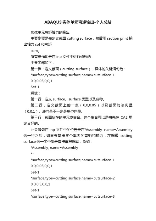
ABAQUS实体单元弯矩输出-个人总结实体单元弯矩轴力的输出主要步骤是先定义截面cutting surface,然后用section print输出轴力sof和弯矩som。
所有操作均是在inp文件中进行修改的主要步骤如下:第一步:定义截面(cutting surface),具体的关键语句为:*surface,type=cutting surface,name=cutsurface-10,0,0.05,0,0,1Set-1解读:第一行,定义surface、surface类型以及名称。
第二行,定义截面上的一点(0,0,0.05)以及截面的法向量(0,0,1)。
法向量不一定是单位向量。
第三行,截面所在的单元或集合。
这个集合可以是事先在CAE里定义好的。
此关键句在inp文件中的位置是在*Assembly, name=Assembly 这一行之后,如果要输出多个截面的弯矩和轴力,在编辑cutting surface这一步中就是直接重复编写,例如:*Assembly, name=Assembly***surface,type=cutting surface,name=cutsurface-10,0,0.05,0,0,1Set-1*surface,type=cutting surface,name=cutsurface-20,0,0.5,0,0,1Set-1*surface,type=cutting surface,name=cutsurface-30,0,1,0,0,1Set-1*surface,type=cutting surface,name=cutsurface-40,0,1.5,0,0,1Set-1*surface,type=cutting surface,name=cutsurface-50,0,1.95,0,0,1Set-1*Instance, name=Part-1-1, part=Part-1第二步:定义输出(section print),具体的关键语句为:*section print,name=forcemoment-1,surface=cutsurface-1,axes=local,frequency=1,update=yessof,som解读:第一行,定义输出的名称及截面。
abaqus提取计算结果
abaqus提取计算结果Abaqus提取计算结果Abaqus是一种广泛使用的有限元分析软件,可以用来模拟和解决各种工程问题。
在使用Abaqus进行分析后,我们需要提取计算结果以便进一步分析和解释。
本文将介绍如何使用Abaqus提取计算结果,并对一些常见的结果进行解释和分析。
一、结果文件的类型和格式在Abaqus中,计算结果以ODB(Output Database)文件的形式保存。
ODB文件是一种二进制文件,包含了计算中生成的各种结果数据,如位移、应力、应变等。
我们可以使用Abaqus提供的odb文件查看器进行结果的可视化和后处理操作。
二、提取计算结果的方法1. 使用Abaqus Python脚本提取结果Abaqus提供了Python脚本接口,可以通过编写脚本来提取计算结果。
以下是一个简单的示例脚本,用于提取位移结果:```pythonfrom abaqus import *from abaqusConstants import *# 打开ODB文件odb = openOdb('job.odb')# 获取位移结果displacementField = odb.steps['Step-1'].frames[-1].fieldOutputs['U']# 输出位移结果displacementField.printValues()```上述脚本首先打开ODB文件,然后获取最后一步的位移结果,并输出到控制台。
2. 使用Abaqus Viewer提取结果除了使用Python脚本,我们还可以使用Abaqus Viewer来手动提取结果。
在Abaqus Viewer中,我们可以选择需要查看和提取的结果类型,并进行相应的后处理操作。
例如,我们可以选择位移结果,并使用矢量图或动画来可视化位移场。
三、常见结果的解释和分析1. 位移结果位移是一种表示结构变形程度的物理量。
在Abaqus中,位移结果可以用箭头图、变形云图等方式进行可视化。
abaqus壳单元截面内力
abaqus壳单元截面内力abaqus是一款强大的有限元分析软件,其壳单元的应用范围广泛,涉及建筑、航空航天、汽车等多个领域。
本文将介绍abaqus壳单元的相关知识,包括壳单元的基本概念、内力分析方法以及在工程应用中的案例解析。
此外,还将探讨如何选择合适的壳单元参数,以提高分析的准确性和效率。
一、Abaqus壳单元简介Abaqus壳单元是基于厚度方向的线性弹性模型来描述壳体的力学行为。
根据壳单元的截面形状,可以分为矩形、圆形、三角形等多种类型。
在abaqus中,壳单元的类型通过关键字“ELAS”指定,如:“*ELAS”。
二、壳单元的内力分析方法在进行壳单元内力分析时,需要考虑壳体的几何参数、材料性能以及边界条件等因素。
abaqus提供了丰富的壳单元内力分析功能,包括线弹性分析、非线性分析等。
分析过程中,可以计算壳体的应力、应变、挠度等参数,为工程设计提供依据。
三、壳单元在工程应用中的案例解析1.飞机翼梁结构分析:利用abaqus壳单元对飞机翼梁进行内力分析,计算梁的弯曲应力、剪切应力以及挠度,评估翼梁结构的强度和刚度。
2.建筑结构分析:采用abaqus壳单元对建筑物的楼板、墙体等进行内力分析,评估建筑结构的稳定性和安全性。
3.汽车车身结构分析:运用abaqus壳单元对汽车车身结构进行碰撞模拟和强度分析,优化车身设计,提高安全性能。
四、如何选择合适的壳单元参数1.选择合适的壳单元类型:根据壳体的几何形状和受力特点,选择合适的壳单元类型,如矩形、圆形等。
2.设置材料性能:为壳单元指定合适的弹性模量、泊松比等材料性能参数。
3.设定边界条件:根据实际工程需求,合理设定壳体的边界条件,如固定边界、滑动边界等。
4.网格划分:合理设置网格密度,平衡计算精度和计算时间。
五、结论与展望abaqus壳单元在工程分析中具有广泛的应用价值。
通过掌握壳单元的分析方法和参数设置,可以有效提高分析结果的准确性和实用性。
abaqus壳单元截面内力
Abaqus壳单元截面内力简介Abaqus是一种强大的有限元分析软件,被广泛用于工程领域中的结构力学分析。
壳单元是Abaqus中常用的一种元素类型,用于模拟薄壳结构的行为。
在壳单元分析中,了解壳单元内力的分布和大小是非常重要的,可以帮助工程师评估结构的稳定性和强度。
本文将介绍如何使用Abaqus进行壳单元截面内力的计算,包括定义壳单元、施加荷载、设置分析步骤和查看结果。
将详细说明每个步骤的操作方法,并提供示例代码和图像来帮助读者更好地理解。
定义壳单元在Abaqus中,壳单元用于模拟薄壳结构的行为。
壳单元可以是平面应力、轴对称或三维应力类型。
在本文中,我们将介绍平面应力的壳单元。
首先,打开Abaqus软件并创建一个新模型。
然后,选择适当的工作平面,例如XY平面。
接下来,选择“Part”模块,并在工作平面上绘制一个封闭的曲线作为壳单元的边界。
确保曲线的方向是逆时针方向,以便正确定义壳单元的正面和背面。
然后,选择“Shell”工具栏中的壳单元类型,例如“Shell181”。
在模型中选择边界曲线,并定义壳单元的厚度和材料属性。
可以根据具体需求,设置不同的壳单元厚度和材料属性。
施加荷载在定义壳单元后,需要施加适当的荷载来模拟实际工况。
在Abaqus中,可以通过定义荷载步骤和荷载边界条件来实现。
首先,选择“Step”模块,并创建一个新的荷载步骤。
在步骤中,可以定义荷载的类型、大小和施加时间。
例如,可以选择静态荷载类型,并定义一个均匀分布的压力荷载。
然后,选择“Load”模块,并创建一个新的荷载边界条件。
在边界条件中,选择适当的载荷类型,例如“Pressure”。
根据实际情况,定义荷载的大小和施加位置。
可以选择在整个壳单元表面施加荷载,或者只在特定区域施加荷载。
设置分析步骤在定义壳单元和施加荷载后,需要设置适当的分析步骤来进行计算。
在Abaqus中,可以选择静态或动态分析步骤,具体取决于所研究问题的性质。
首先,选择“Step”模块,并创建一个新的分析步骤。
abaqus第二讲:ABAQUS中的实体单元解析
受弯矩M作用下完全积分、二次单元的变形
北京怡格明思工程技术有限公司
Innovating through simulation
只有当确信载荷只会在模型中产生很小的弯曲时,才可以采用完全 积分的线性单元。 如果对载荷产生的变形类型有所怀疑,则应采用不同类型的单元。 在复杂应力状态下,完全积分的二次单元也有可能发生自锁;因此, 如果在模型中应用这类单元,应细心地检查计算结果。 然而,对于模拟局部应力集中的区域,应用这类单元是非常有用的!
北京怡格明思工程技术有限公司
Innovating through simulation
ABAQUS中的单元
公式(又称数学描述)
• 用于描述单元行为的数学公式是用于单元分类的另一种方法。 • 不同单元公式的例子: 平面应变 平面应力 杂交单元 非协调元 小应变壳 有限应变壳 厚壳 薄壳
北京怡格明思工程技术有限公司
受弯矩M作用下材料的变形 线性单元的边不能弯曲;所以,如果应用单一单元来模拟这一小块材料, 其变形后的形状如图所示。
受弯矩M作用下完全积分、线性单元的变形
北京怡格明思工程技术有限公司
Innovating through simulation
为清楚起见,画出了通过积分点的虚线。显然,上部虚线的长度增加,说明1方向的 应力是拉伸的。类似地,下部虚线的长度缩短,说明是压缩的。竖直方向虚线的长 度没有改变(假设位移是很小的);所有这些都与受纯弯曲的小块材料应力的预期 状态是一致的。但是,在每一个积分点处,竖直线与水平线之间夹角开始时为90度, 变形后却改变了,说明这些点上的剪应力不为零。显然,这是不正确的:在纯弯曲 时,这一小块材料中的剪应力应该为零。 产生这种伪剪应力的原因是因为单元的边不能弯曲,它的出现意味着应变能正在产 生剪切变形,而不是产生所希望的弯曲变形,因此总的挠度变小:即单元是过于的 刚硬。 剪力自锁仅影响受弯曲载荷的完全积分的线性单元的行为。在受轴向或剪切载荷时, 这些单元的功能表现很好。而二次单元的边界可以弯曲,故它没有剪力自锁的问题。 二次单元预测的自由端位移接近于理论解答。
abaqus壳单元截面内力 -回复
abaqus壳单元截面内力-回复题目:Abaqus壳单元截面内力分析引言:Abaqus是一种广泛应用于工程领域的有限元软件,其在结构分析中具有广泛的应用。
对于壳单元来说,内力分析是其中一个重要的工作,它能够提供重要的结构设计和分析依据。
本文将一步一步介绍如何使用Abaqus 进行壳单元截面内力分析。
第一步:模型建立在Abaqus中,首先需要建立一个合适的模型。
在建模过程中,需要考虑结构的几何形状和材料特性等因素。
通过选择合适的壳单元类型、节点布置以及边界条件等,可以建立一个具有实际工程意义的模型。
第二步:设置截面属性在Abaqus中,壳单元的截面属性可以通过截面集(Section)进行定义。
通过选择合适的截面类型,可以指定壳单元的几何形状和截面特性等参数。
在定义截面属性时,可以根据实际需要选择材料类型、厚度、弹性模量、剪切模量等参数。
第三步:应用载荷和约束在实际工程中,结构往往会受到外部载荷的作用。
在Abaqus中,可以通过施加节点载荷、边界条件和约束等方式来模拟不同的工况。
在进行壳单元截面内力分析时,需要定义合适的载荷和边界条件。
例如,可以施加集中力、分布力、压力或者转矩等载荷,并通过边界条件限制结构的自由度。
第四步:网格划分和求解在完成模型的建立、截面属性的设置以及载荷与约束的施加后,需要进行网格划分和求解。
Abaqus使用有限元法进行问题求解,通过将结构划分为一些小的单元来近似描述结构的变形和应力分布。
通过合理选择网格划分的参数,可以获得合适的计算精度。
第五步:结果输出和分析在求解过程完成后,Abaqus会生成一系列关于结构的分析结果。
这些结果包括节点位移、应力、应变、内力等信息。
通过对这些结果进行后处理,可以得到结构的详细内力分布情况。
此外,Abaqus还提供了可视化的工具,可以将结果以图表形式进行展示和分析。
结论:本文基于Abaqus软件,详细介绍了壳单元截面内力分析的步骤。
通过模型建立、截面属性设置、载荷与约束施加、网格划分和求解,以及结果输出与分析等步骤,可以获得结构内力分布的详细信息。
abaqus壳单元截面内力

abaqus壳单元截面内力壳单元是ABAQUS软件中的一种元素类型,用于模拟薄壳结构的行为,包括板、膜、薄壳等结构。
在ABAQUS中,壳单元可以用来分析结构在载荷作用下的应力分布,以及在不同载荷下的变形情况。
截面内力是指壳单元在载荷作用下,各个截面上的应力分布情况。
在ABAQUS中,可以通过截面内力的计算来了解壳单元在不同点上的受力情况,并根据这些数据来进行结构的设计和优化。
壳单元的截面内力可以用多种方式来表示和计算,常见的有平均应力法和高斯积分法。
平均应力法是指通过将截面等分为若干个小矩形区域,然后在每个小矩形区域上计算应力,最后将这些应力求平均得到整个截面的平均应力。
高斯积分法是指通过在截面上选择一系列高斯积分点,然后在每个积分点上计算应力,最后将所有积分点上的应力进行加权求和得到整个截面的应力分布。
对于ABAQUS中的壳单元,通常可以选择线性弯曲、非线性弯曲和混合弯曲等不同的假设来进行计算。
线性弯曲是指假设壳单元在受载时产生的应力与由平衡方程和应变-位移关系所得到的应力具有线性关系,非线性弯曲是指考虑应变偏离线性范围时的非线性效应,混合弯曲则是综合考虑线性和非线性效应。
在ABAQUS中,可以通过定义截面属性来描述壳单元的截面特性,如截面厚度、截面形状等。
通过定义合适的截面属性,可以准确地模拟壳单元在载荷作用下的行为。
对于截面内力的计算,可以通过ABAQUS中提供的后处理工具来进行。
在后处理中,可以选择某个特定的截面,并查看该截面上的应力和应变分布。
通过分析这些数据,可以了解到壳单元在截面上的受力情况,进而进行后续的工程设计和分析。
总的来说,ABAQUS的壳单元截面内力计算是一种用于分析薄壳结构行为的有效方法。
通过合理地定义截面属性和选择适当的计算方法,可以得到准确的截面内力数据,为结构设计和优化提供重要依据。
ABAQUS常用技巧归纳图文并茂
ABAQUS常用技巧归纳图文并茂ABAQUS常用技巧归纳一、背景介绍ABAQUS是一款广泛应用于工程领域的有限元分析软件,具备强大的功能和丰富的工具包,被工程师广泛使用。
然而,在使用ABAQUS的过程中,我们经常会遇到一些技巧和问题,本文将针对一些常见的ABAQUS技巧进行归纳总结,帮助读者更好地应用ABAQUS进行工程分析。
二、常用技巧1. 单元类型选择在使用ABAQUS进行有限元分析时,选择合适的单元类型是非常重要的。
根据具体的分析对象和问题类型,可以选择不同的单元类型,如线性单元、非线性单元或复合单元。
合理的单元选择可以提高计算效率和分析精度。
2. 网格划分优化合理的网格划分对计算结果的准确性和计算效率至关重要。
在ABAQUS中,提供了多个网格划分工具和算法,可以帮助用户进行网格优化。
例如,使用网格生成工具可以自动生成符合几何形状和尺寸要求的网格,使用网格划分工具可以调整网格的密度和精度。
3. 材料模型选择在ABAQUS中,提供了多种材料模型,用于描述材料的力学行为。
根据具体的分析对象和材料性质,可以选择合适的材料模型,如线性弹性模型、塑性模型或粘弹性模型。
合理的材料模型选择可以更好地模拟材料的本构行为。
4. 边界条件设置在有限元分析中,正确设置边界条件是保证结果准确性的关键。
在ABAQUS中,可以通过节点约束、荷载施加和接触定义等方式来设置边界条件。
应根据具体的分析问题和工况设置合理的边界条件,以确保计算结果的可靠性。
5. 后处理及结果分析ABAQUS提供了强大的后处理和结果分析功能,可以帮助用户深入理解计算结果。
通过后处理工具,可以对计算结果进行可视化分析、曲线绘制和云图展示等,帮助用户对结果进行全面的评估和解读。
6. 自定义脚本开发除了使用ABAQUS内置的工具和功能,用户还可以通过编写脚本来定制化分析过程。
ABAQUS支持Python脚本的开发和调用,用户可以利用脚本进行批处理、参数化分析和复杂算法实现等。
- 1、下载文档前请自行甄别文档内容的完整性,平台不提供额外的编辑、内容补充、找答案等附加服务。
- 2、"仅部分预览"的文档,不可在线预览部分如存在完整性等问题,可反馈申请退款(可完整预览的文档不适用该条件!)。
- 3、如文档侵犯您的权益,请联系客服反馈,我们会尽快为您处理(人工客服工作时间:9:00-18:30)。
实体单元建的模型,要提取截面的内力有什么好方法呢?我看过别人的一个帖:对于一般的实体单元结构可以定义surface 然后用section file 输出其中,这个surface可以在cae中定义,也可以在inp中定义,但是由于涉及到边的编号问题,所以在inp中容易出错。
section file 的结果直接在dat中可见。
需要编制小程序将其数据提取。
一定要编个程序才可以提取吗在dat文件里没有找到什么section file是输出在*.fil文件中。
要直接得到截面的total force,moment,heat flux可以在inp中添加:*SECTION PRINT,name=*,surface=**SOF,SOM在dat文件中可以找到总内力和弯矩我做钢筋混凝土的问题,模型分为两个part,分别是钢筋和混凝土,然后Assembe在一起,将钢筋embeded到混凝土内。
我在keywords编辑器End assemble前定义*surface, type=cutting surface,name=surface_1-21.5,0,0,1,0,0怎么也不成,总说定义的截面没有相交(坐标计算没有错误)。
第三行空着(帮助文档说表示截断整个模型)也不行,写上钢筋或混凝土的单元组名(没有另建组,直接用的keywords编辑器中钢筋或混凝土生成单元的组名)也不行。
请问是怎么回事?哪位有相关的例子给我一个,我的QQ:40735053。
还望不吝赐教,谢谢。
Displaying a free body cutYou can define a free body cut to view the resultant forces and moments transmitted across a selected surface of a model. Force vectors are displayed with a single arrowhead and moment vectors with a double arrowhead.To create a free body cut:1. To display the entire model in the viewport, select Tools Display Group Plot All fromthe main menu bar.2. From the main menu bar, select Tools Free Body Cut Manager.3. Click Create in the Free Body Cut Manager.4. From the dialog box that appears, select 3D element faces as the Selection method andclick Continue.5. In the Free Body Cross-Section dialog box, select Surfaces as the Item and Pick fromviewport as the Method.6. In the prompt area, set the selection method to by angle and accept the default angle.7. Select the surface, highlighted in Figure 4–33, to define the free body cut cross-section.a. From the Selection toolbar, toggle off the Select the Entity Closest to theScreen tool and ensure that the Select From All Entities tool is selected.b. As you move the cursor in the viewport, Abaqus/CAE highlights all of the potentialselections and adds ellipsis marks (...) next to the cursor arrow to indicate an ambiguousselection. Position the cursor so that one of the faces of the desired surface ishighlighted, and click to display the first surface selection.Figure 4–33 Selected faces for the free body cross-section.c. Use the Next and Previous buttons to cycle through the possible selections until theappropriate vertical surface is highlighted, and click OK.8. Click Done in the prompt area to indicate your selection is complete. Click OK in the FreeBody Cross-Section dialog box.9. In the Edit Free Body Cut dialog box, accept the default settings for the SummationPoint and the Component Resolution. Click OK to close the dialog box.10. Click Options in the Free Body Cut Manager.11. From the Free Body Plot Options dialog box, select the Force tab in the Color &Style tabbed page. Click the resultant color sample to change the color of the resultant force arrow.12. Once you have selected a new color for the resultant force arrow, click OK in the Free BodyPlot Options dialog box and click Dismiss in the Free Body Cut Manager.The free body cut is displayed in the viewport, as shown in Figure 4–34.Figure 4–34 Free body cut displayed on the connecting lug.Generating tabular data reports for subsets of the modelTabular output data were generated earlier for this model using printed output requests. However, for complicated models it is convenient to write these data for selected regions of the model using Abaqus/Viewer. This is achieved using display groups in conjunction with the report generation feature. For the connecting lug problem we will generate the following tabular data reports: •Stresses in the elements at the built-in end of the lug (to determine the maximum stress in the lug)•Reaction forces at the built-in end of the lug (to check that the reaction forces at the constraints balance the applied loads)•Vertical displacements at the bottom of the hole (to determine the deflection of the lug when the load is applied)Each of these reports will be generated using display groups whose contents are selected in the viewport. Thus, begin by creating and saving display groups for each region of interest.To create and save a display group containing the elements at the built-in end:1. In the Results Tree, double-click Display Groups.2. Choose Elements from the Item list and Pick from viewport as the selection method.3. Restore the option to select entities closest to the screen.4. In the prompt area, set the selection method to by angle; and click the built-in face of the lug.Click Done when all the elements at the built-in face of the lug are highlighted in the viewport.In the Create Display Group dialog box, click Replace followed by Save As. Save thedisplay group as built-in elements.To create and save a display group containing the nodes at the built-in end:1. In the Create Display Group dialog box, choose Nodes from the Item list and Pick fromviewport as the selection method.2. In the prompt area, set the selection method to by angle; and click the built-in face of the lug.Click Done when all the nodes on the built-in face of the lug are highlighted in the viewport. In the Create Display Group dialog box, click Replace followed by Save As. Save thedisplay group as built-in nodes.To create and save a display group containing the nodes at the bottom of the hole:1. In the Create Display Group dialog box, select All from the item list, and click Replace toreset the active display group to include the entire model.2. In the Create Display Group dialog box, choose Nodes from the Item list and Pick fromviewport as the selection method.3. In the prompt area, set the selection method to individually; and select the nodes at thebottom of the hole in the lug, as indicated in Figure 4–35. Click Done when all the nodes on the bottom of the hole are highlighted in the viewport. In the Create Display Group dialog box,click Replace followed by Save As. Save the display group as nodes at hole bottom.Figure 4–35 Nodes in display group nodes at hole bottom.Now generate the reports.To generate field data reports:1. In the Results Tree, click mouse button 3 on built-in elements underneath the DisplayGroups container. In the menu that appears, select Plot to make it the current display group.2. From the main menu bar, select Report Field Output.3. In the Variable tabbed page of the Report Field Output dialog box, accept the default positionlabeled Integration Point. Click the triangle next to S: Stress components to expand the list of available variables. From this list, select Mises and the six individual stresscomponents: S11, S22, S33, S12, S13, and S23.4. In the Setup tabbed page, name the report Lug.rpt. In the Data region at the bottom of thepage, toggle off Column totals.5. Click Apply.6. In the Results Tree, click mouse button 3 on built-in nodes underneath the DisplayGroups container. In the menu that appears, select Plot to make it the current display group.(To see the nodes, toggle on Show node symbols in the Common Plot Options dialog box.)7. In the Variable tabbed page of the Report Field Output dialog box, change the positionto Unique Nodal. Toggle off S: Stress components, and select RF1, RF2, and RF3 from the list of available RF: Reaction force variables.8. In the Data region at the bottom of the Setup tabbed page, toggle on Column totals.9. Click Apply.10. In the Results Tree, click mouse button 3 on nodes at hole bottom underneath the DisplayGroups container. In the menu that appears, select Plot to make it the current display group.11. In the Variable tabbed page of the Report Field Output dialog box, toggle off RF: Reactionforce, and select U2 from the list of available U: Spatial displacement variables.12. In the Data region at the bottom of the Setup tabbed page, toggle off Column totals.13. Click OK.Open the file Lug.rpt in a text editor. A portion of the table of element stresses is shown below. The element data are given at the element integration points. The integration point associated with a given element is noted under the column labeled Int Pt. The bottom of the table contains information on the maximum and minimum stress values in this group of elements. The results indicate that the maximum Mises stress at the built-in end is approximately 330 MPa. Your results may differ slightly if your mesh is not identical to the one used here.*SECTION PRINTDefine print requests of accumulated quantities on user-defined surface sections.This option is used to provide tabular output of accumulated quantities associated with a user-defined section. Depending on the analysis type the output may include one or several of the following: the total force, the total moment, the total heat flux, the total current, the total mass flow, or the total pore fluid volume flux associated with the section. This option is not available for eigenfrequency extraction, eigenvalue buckling prediction, complex eigenfrequency extraction, or linear dynamics procedures.Product: Abaqus/StandardType: History dataLevel: StepReferences:•“Output to the data and results files,”Section 4.1.2 of the Abaqus Analysis User's Manual •“Abaqus/Standard output variable identifiers,”Section 4.2.1 of the Abaqus Analysis User's ManualRequired parameters:NAMESet this parameter equal to a label that will be used to identify the output for the section. Section names in the same input file must be unique.SURFACESet this parameter equal to the name used in the *SURFACE option to define the surface.Optional parameters:AXESFREQUENCYSet this parameter equal to the output frequency, in increments. The output will always be printed at the last increment of each step unlessFREQUENCY=0. The default is FREQUENCY=1.Set FREQUENCY=0 to suppress the output.UPDATESet UPDATE=NO if output is desired in the original local system of coordinates.Set UPDATE=YES (default) to output quantities in a local system of coordinates that rotates with the average rigid body motion of the surface section. This parameter is relevant only ifAXES=LOCAL and the NLGEOM parameter is active in the step.Optional data lines:First line:1. Node number of the anchor point (blank if coordinates given).2. First coordinate of the anchor point (ignored if node number given).3. Second coordinate of the anchor point (ignored if node number given).4. Third coordinate of the anchor point (for three-dimensional cases only; ignored if node numbergiven).Leave this line blank to allow Abaqus to define the anchor point.Second line:1. Node number used to specify point a in Figure 18.5–1 (blank if coordinates given).2. First coordinate of point a (ignored if node number given).3. Second coordinate of point a (ignored if node number given).The remaining data items are relevant only for three-dimensional cases.4. Third coordinate of point a (ignored if node number given).5. Node number used to specify point b (blank if coordinates given)6. First coordinate of point b (ignored if node number given).7. Second coordinate of point b (ignored if node number given).8. Third coordinate of point b (ignored if node number given).Leave this line blank to allow Abaqus to define the axes.Third line:Figure 18.5–1 User-defined local coordinate system.SOFTotal force in the section..dat: yes .fil: yes .odb Field: no .odb History: noSOMTotal moment in the section..dat: yes .fil: yes .odb Field: no .odb History: noSOCFCenter of the total force in the section..dat: yes .fil: yes .odb Field: no .odb History: no24.4实体单元的截面力/弯矩/转角[url=/forum/viewthread.php?tid=724857]/forum/viewthread.php tid=724857[/url]问:求助:请问abaqus里面怎样看一个构件截面(如:钢骨混凝土压弯柱)的内力啊请问:SRC柱模拟后,如何提取截面内力:如某一截面处的轴力、弯矩、剪力等内容,谢谢。