MATLAB与控制系统仿真及实验 2016 (二)
MATLAB语言与控制系统仿真实验

MATLAB语言与控制系统仿真实验报告册姓名:班级:学号:日期:实验一 MATLAB/Simulink 仿真基础一、 实验目的1、 掌握MATLAB/Simulink 仿真的基本知识;2、能在Simulink 中实现简单模型的搭建。
二、 实验工具电脑、MATLAB 软件三、 实验内容1、绘制衰减曲线)3sin(.3t e y t -=及其包络30t e y -±=,其中]4,0[π∈t 。
2、用MATLAB 实现运算5ln 573sin 3+++=e y3、用simulink 建立subsystem 并封装,内容为正弦波发生器)sin(ϕω+=t A y ,要求幅值、频率和初相任意可调。
4、用simulink 实现下列程序语句: Int C=0;If 0≥-B A ; C++; Else C--。
四、实验过程1t=0:pi/50:4*pi;y=exp(-t/3).*sin(3*t); y0=exp(-t/3);plot(t,y,'c',t,y0,'b:',t,-y0,'b:'); axis([0 4*pi -1 1]); title('函数图形'); xlabel('时间/t') ylabel('幅值');legend('衰减曲线','包络线');2 y=sin(3)+sqrt(7)+5*exp(3)+log(5)y =104.82403五、实验结论1衰减曲线包络线值幅时间/t2 y = 104.824034实验二控制系统模型的MATLAB实现四、实验目的3、掌握MATLAB/Simulink仿真的基本知识;4、熟练应用MATLAB软件建立控制系统模型。
五、实验工具电脑、MATLAB软件六、实验内容已知单位负反馈控制系统开环传递函数为)1)(5()(++=As s s Bs G ,其中,A表示自己学号最后一位数(可以是零),B 表示自己学号的最后两位数。
《Matlab与控制系统仿真》实验指导书

机械与汽车工程学院《Matlab控制系统仿真》实验指导书学院班级姓名学号浙江科技学院机械与汽车工程学院制实验一 MATLAB语言基本命令1 实验目的1. 掌握科学计算的有关方法,熟悉MA TLAB语言及其在科学计算中的运用;2. 掌握MATLAB的命令运行方式和M文件运行方式;3. 掌握矩阵在MA TLAB中的运用。
2 实验器材计算机WinXP、Matlab7.0软件3 实验内容(1). 输入A=[7 1 5;2 5 6;3 1 5],B=[1 1 1; 2 2 2;3 3 3],在命令窗口中执行下列表达式,掌握其含义:A(2, 3) A(:,2) A(3,:) A(:,1:2:3)A(:,3).*B(:,2) A(:,3)*B(2,:) A*B A.*BA^2 A.^2 B/A B./A(2).输入C=1:2:20,则C(i)表示什么?其中i=1,2,3, (10)(3).查找已创建变量的信息,删除无用的变量;(4). 试用help命令理解下面程序各指令的含义:cleart =0:0.001:2*pi;subplot(2,2,1);polar(t, 1+cos(t))subplot(2,2,2);plot(cos(t).^3,sin(t).^3)subplot(2,2,3);polar(t,abs(sin(t).*cos(t)))subplot(2,2,4);polar(t,(cos(2*t)).^0.5)4 实验步骤:打开MA TLAB程序,将实验内容中的题目依次输入MATLAB中,运行得到并记录结果,最后再对所得结果进行验证。
5 实验报告要求记录实验数据,理解其含义实验二 MATLAB语言程序设计1 实验目的(1)掌握Matlab程序的编制环境和运行环境。
(2)掌握Matlab程序的编写方法。
(3)能编写基本的数据处理Matlab程序。
(4)能编写基本的数据可视化Matlab程序。
2 实验器材计算机WinXP、Matlab7.0软件3 实验内容(1) Matlab脚本文件编写和执行(2) Matlab 函数文件的编写和调用(3) nargm和nargout函数使用方法(4) 局部变量与全局变量使用4 实验步骤1、Matlab命令文件编写(1) 建立自己工作目录,如/Mywork。
MATLAB与控制系统仿真实验书

实验总要求1、封面必须注明实验名称、实验时间和实验地点,实验人员班级、学号(全号)和姓名等。
2、内容方面:注明实验所用设备、仪器及实验步骤方法;记录清楚实验所得的原始数据和图像,并按实验要求绘制相关图表、曲线或计算相关数据;认真分析所得实验结果,得出明确实验结论。
3、图形可以打印出来并剪贴上去,文字必须用标准试验纸手写。
实验一MATLAB绘图基础一、实验目的了解MATLAB常用命令和常见的内建函数使用。
熟悉矩阵基本运算以及点运算。
掌握MATLAB绘图的基本操作:向量初始化、向量基本运算、绘图命令plot,plot3,mesh,surf 使用、绘制多个图形的方法。
二、实验内容建立并执行M文件multi_plot.m,使之画出如图的曲线。
三、实验方法(参考程序)024681012Plot of y=sin(2x) and its derivative四、实验要求1. 分析给出的MA TLAB 参考程序,理解MA TLAB 程序设计的思维方法及其结构。
2. 添加或更改程序中的指令和参数,预想其效果并验证,并对各语句做出详细注释。
对不熟悉的指令可通过HELP 查看帮助文件了解其使用方法。
达到熟悉MA TLAB 画图操作的目的。
3. 总结MATLAB 中常用指令的作用及其调用格式。
五、实验思考1、实现同时画出多图还有其它方法,请思考怎样实现,并给出一种实现方法。
(参考程序如下)t=0:pi/100:4*pi;y1=sin(2*t);y2=2*cos(2*t);plot(t,y1,'-b');hold on; %保持原图plot(t,y2,'-g');grid onaxis([0 4*pi -2 2])title('Plot of y=sin(2x) and its derivative')Plot of y=sin(2x) and its deriv ativ e024681012024681012-2-1012xyPlot of y=sin(2x)024681012-2-1012xyPlot derivative of y=sin(2x);y=2cos(2x)t=0:pi/100:4*pi; y1=sin(2*t); y2=2*cos(2*t);024681012-2-1.5-1-0.500.511.52Plot of y=sin(2x) and its deriv ativ et=0:pi/100:4*pi; y1=sin(2*t); y2=2*cos(2*t); plot(t,y1,'r--'); hold on ;plot(t,y2,'-b'); grid onaxis([0 4*pi -2 2])title('Plot of y=sin(2x) and its derivative')2468101214Plot of y=sin(2x)xyPlot of y=sin(2x) and its deriv ativ exyt=0:pi/100:4*pi; y1=sin(2*t); y2=2*cos(2*t); plot(t,y1,'r--');title('Plot of y=sin(2x)'); xlabel('x'),ylabel('y'); figure(2) plot(t,y2,'-b');title('Plot of y=sin(2x) and its derivative') xlabel('x'),ylabel('y'); grid onaxis([0 4*pi -2 2])2、思考三维曲线(plot3)与曲面(mesh, surf)的用法,(1)绘制参数方程233,)3cos(,)3sin()(t z e t t y e t t t x t t ===--的三维曲线;t=0:pi/30:10*pi;plot3(t.^3.*sin(3.*t).*exp(-t),t.^3.*cos(3.*t).*exp(-t),t.^2);2(2)绘制二元函数xyy xe x x y xf z ----==22)2(),(2,在XOY 平面内选择一个区域(-3:0.1:3,-2:0.1:2),然后绘制出其三维表面图形。
《MATLAB与控制系统仿真》实验报告
《MATLAB与控制系统仿真》实验报告一、实验目的本实验旨在通过MATLAB软件进行控制系统的仿真,并通过仿真结果分析控制系统的性能。
二、实验器材1.计算机2.MATLAB软件三、实验内容1.搭建控制系统模型在MATLAB软件中,通过使用控制系统工具箱,我们可以搭建不同类型的控制系统模型。
本实验中我们选择了一个简单的比例控制系统模型。
2.设定输入信号我们需要为控制系统提供输入信号进行仿真。
在MATLAB中,我们可以使用信号工具箱来产生不同类型的信号。
本实验中,我们选择了一个阶跃信号作为输入信号。
3.运行仿真通过设置模型参数、输入信号以及仿真时间等相关参数后,我们可以运行仿真。
MATLAB会根据系统模型和输入信号产生输出信号,并显示在仿真界面上。
4.分析控制系统性能根据仿真结果,我们可以对控制系统的性能进行分析。
常见的性能指标包括系统的稳态误差、超调量、响应时间等。
四、实验步骤1. 打开MATLAB软件,并在命令窗口中输入“controlSystemDesigner”命令,打开控制系统工具箱。
2.在控制系统工具箱中选择比例控制器模型,并设置相应的增益参数。
3.在信号工具箱中选择阶跃信号,并设置相应的幅值和起始时间。
4.在仿真界面中设置仿真时间,并点击运行按钮,开始仿真。
5.根据仿真结果,分析控制系统的性能指标,并记录下相应的数值,并根据数值进行分析和讨论。
五、实验结果与分析根据运行仿真获得的结果,我们可以得到控制系统的输出信号曲线。
通过观察输出信号的稳态值、超调量、响应时间等性能指标,我们可以对控制系统的性能进行分析和评价。
六、实验总结通过本次实验,我们学习了如何使用MATLAB软件进行控制系统仿真,并提取控制系统的性能指标。
通过实验,我们可以更加直观地理解控制系统的工作原理,为控制系统设计和分析提供了重要的工具和思路。
七、实验心得通过本次实验,我深刻理解了控制系统仿真的重要性和必要性。
MATLAB软件提供了强大的仿真工具和功能,能够帮助我们更好地理解和分析控制系统的性能。
MATLAB仿真实验实验内容(2016)_32457
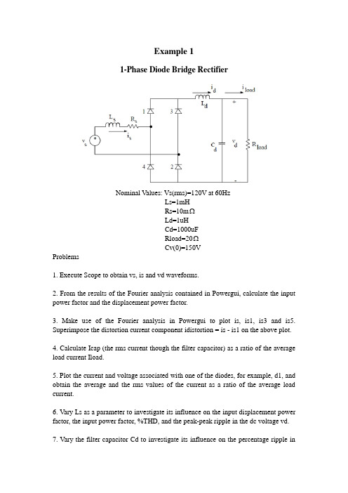
Example 11-Phase Diode Bridge RectifierNominal Values: Vs(rms)=120V at 60HzLs=1mHRs=10mΩLd=1uHCd=1000uFRload=20ΩCv(0)=150VProblems1. Execute Scope to obtain vs, is and vd waveforms.2. From the results of the Fourier analysis contained in Powergui, calculate the input power factor and the displacement power factor.3. Make use of the Fourier analysis in Powergui to plot is, is1, is3 and is5. Superimpose the distortion current component idistortion = is - is1 on the above plot.4. Calculate Icap (the rms current though the filter capacitor) as a ratio of the average load current Iload.5. Plot the current and voltage associated with one of the diodes, for example, d1, and obtain the average and the rms values of the current as a ratio of the average load current.6. Vary Ls as a parameter to investigate its influence on the input displacement power factor, the input power factor, %THD, and the peak-peak ripple in the dc voltage vd.7. Vary the filter capacitor Cd to investigate its influence on the percentage ripple invd, input displacement power factor and %THD. Plot the percentage ΔVd (peak-to-peak) / Vd (average) as a function of Cd.8. Vary the load power to investigate its influence on the average dc voltage.9. Obtain the vs, is and vd waveforms during the startup transient when the filter capacitor is initially not charged. Obtain the peak inrush current as a ratio of the peak current in steady state. Vary the switching instant by simply varying the phase angle θof the source vs. (Hint: change Cv(0)=150V to Cv(0)=0V)10. Replace the dc side of the diode bridge by a current source I d=10A, corresponding to a very large Ld . Make Ls almost equal to zero. Obtain Vd(average).11.Make Ls=3 mH in Problem 9 and obtain Vd (average), displacement power factor, power factor, %THD.Example 23-Phase Diode Bridge RectifierNominal Values: V LL(rms)=208V at 60HzLs=0.1mHRs=1mΩLd=0.5mHRd=5mΩCd=500uFRload=16.5ΩProblems:1. (a)Obtain v ab, v d and i d waveforms.(b)Obtain v a and i a waveforms2. By means of Fourier analysis of ia, calculate its harmonic components as a ratio of Ia1.3. Calculate Ia, Ia1, Idis, %THD in the input current, input displacement power factor and the input power factor. How do the results compare with the 1-phase diode-bridge rectifier of Example 1.4. Calculate Icap(the rms current through the filter capacitor) as a ratio of the average load current Iload. Compare the results with that in Example 1.5. Investigate the influence of Ld on the input displacement power factor, the input power factor and the average dc voltage Vd. Suggested range of Ld: 0.1 mH to 10 mH.6. Investigate the influence of Cd on the percent ripple in vd. Plot the percentage ΔVd(peak-to-peak)/Vd(average) as a function of Cd. Suggested range of Cd: 100uF and 2,000uF.7. Investigate the influence of Cd on the input displacement power factor and the input power factor. Suggested range of Cd: 100μF to 2,000μF.8. Plot the average dc voltage as a function of load. Suggested range of R load: 50Ω to 8Ω.Example 53-Phase Thyristor Rectifier BridgeNominal Values: V LL (rms)=208V at 60HzLs1=0.2mHLs2=1mHLd=16mHRload=16.5Ωdelay angle=45°Problems1. (a) Obtain va, vd and id waveforms using Scope.(b) Obtain va and ia waveforms.(c) Obtain (va)pcc, (vab)pcc and ia waveforms.2. From the plots, obtain the commutation interval u and id at the start of the commutation. Verify the following commutation equation:2cos()cos 2s d LL L u I V ωαα+=−where Ls = Ls1 + Ls2. For Id, use the average value of id or its value at the start of the commutation.3. By means of Fourier analysis of is, calculate its harmonic components as a ratio of Is1.4. Calculate Is, %THD in the input current, the input displacement power factor and the input power factor.5. Verify the following equation:Displacement power factor cos cos()cos()22uu ααα++≅+≅6. At the point of common coupling, obtain the following from the voltage v pccwaveform:(a) Line-notch depth ρ(%)(b) Line-notch area and,(c) voltage THD%.7. Obtain the average dc voltage Vd. Verify that31.35cos sd LL d L V V I ωαπ=−For Id, use the average value of id or its value at the start of the commutation.3-Phase Thyristor InverterNominal Values: V LL(rms)=480V at 60HzLs=0.1mHLd=16mHRd=1ΩE=480Vdelay angle α=160°Problems:1. (a) Obtain va , vd and id waveforms using scope.(b) Obtain va and ia waveforms2. Calculate Is, %THD in the input current, the input displacement power factor and the input power factor.3. Study the startup of the inverter operation. Increase the delay angle to a value close to 180° and look at the va, vd and id waveforms. Repeat the above procedure by reducing αslowly to its nominal value of 160°. Plot the average dc current Id versus α.Step-down (BUCK) dc-dc ConverterNominal Values: V d =8V(dc)L=5uHrL=10m ΩC=100uFRload=0.5Ωfs=100kHzswitch duty ratio D=0.75Problems1. In steady state, obtain the following waveforms using Scope:(a) vL and iL waveforms.(b) vo, iL and ic waveforms2. Obtain voi waveform and by means of Fourier analysis, obtain its harmonic components as a ratio of its average value V o.3. Increase the load resistance to 10Ω. Obtain vL and iL waveforms in the discontinuous conduction mode [Hint: use V(0)=5.8V and I L (0)=0]. Check if the results agree with the following equation:22,max 1()4o o d LB V D I V D I =+ Where ,max 8d LB sV I Lf = . 4. Obtain the peak-to-peak ripple in the output voltage and check to see if the results agree with the analytical calculations.5. Calculate the rms value of the current through the output capacitor as a ratio of theaverage load current Io.6. Calculate the peak-to-peak ripple in the output voltage in the presence of the output capacitor Equivalent Series Resistance (ESR)[Suggested ESR=100mΩ]. Plot the ripple across C, ESR and the total ripple in vo.Example 10Full-Bridge, Bipolar-Switching dc-dc ConverterNominal Values: V d=200VV EMF=79.5VRa=0.37ΩLa=1.5mHIo(avg)=10Afs=20kHzswitch duty ratio D1 of T A1 and T B2=0.708(so v control=0.416V with Vtri=1.0V)Problems:1. Obtain the following waveforms using Scope:(a) vo, io and po(t) = vo*io(b) vo and id2. Calculate peak-to-peak ripple in io.3. By means of Fourier analysis, calculate the average value and the harmonic components in vo. Obtain the rms value of the ripple in vo and check it with theanalytical calculations.4. By means of Fourier analysis, calculate the average value of id and the rms value ofthe ripple.5. With V EMF=0 and Ia(avg)=0, V o(avg)=0V. Therefore, Vcontrol=0. Calculate thefollowing [Hint: use Io(0)=-1.67A]:(a) vo, ioand po(t) waveforms.(b) peak-to-peak ripple in io. Compare it with its analytical value, and that in Problem 2.(c) In part (a), label the intervals during which various devices are conducting.6. In the regenerative mode, the power flows from the load to the dc-bus at Vd. Let V EMF =79.5V , Ia(avg)=10A in the reverse direction, and V o(avg)=79.5-0.37×10=75.8V . Therefore,75.8 1.00.379200control V =×= Calculate parts (a) through (c) of Problem 5 [Hint: use Io(0)=-11.67 A].Example 121-Phase, Bipolar-Voltage Switching InverterNominal Values: Frequency f1=40Hz, V o1(rms)=153.33V, V o1(peak)=216.8V.R TH=2Ω, L TH=10mH. Io1(rms)=10A at a 0.866 pf (lagging)Therefore, V TH(rms)=124.1 5.39∠−°Vand v TH=175.5sin(2π*40t-5.39°).Inverter and Controller for Sinusoidal PWM:Switching frequency fs=1kHz,Frequency modulation ratio m f=1000/40=25;Amplitude modulation ratio m a=0.8.Therefore, Vd=Vo1, peak/m a=271 V and,v control=0.8sin(2π*40t).Problems:1. Obtain the following waveforms using Scope:(a) vo and io.(b) vo and id.(c) vo, io and po.2. Obtain vo1 by means of Fourier analysis of the vo waveform. Compare vo1 with its precalculated nominal value.3. Using the results of Problem 2, obtain the ripple component v,ripple waveform in the output voltage.4. Obtain io1 by means of Fourier analysis of the io waveform. Compare io1 with its precalculated nominal value.5. Using the results of Problem 4, obtain the ripple component i,ripple in the output current.6. Obtain Id(avg) and id2 (the component at the 2nd harmonic frequency) by means of the Fourier analysis of the id waveform. Compare them with their precalculated nominal values.ing the results of Problem 6, obtain the high frequency ripple componentid,ripple in the input dc current. Calculate its rms value.Based on Io1(rms)=1030∠o A, the initial value Io(0)=-7A.-Example 16Three-Phase PWM InverterNominal Values:Load: A 230V ,60Hz, 3-phase motor is operating at a frequency f 1=47.619Hz. Therefore,147.619230182.54V 60rms LL V =×= 11105.39V=105.3903rms LL rmsAn V V ==∠°110A rms A I =at a lagging power factor of 0.8661030A =∠−° Rs=2Ω, Ls=10mH,Xs=3247.61910103π−×××=Ω(V TH ,A )1=74.7612.36V(rms)∠−°Inverter and Controller for Sinusoidal PWM:Switching frequency fs=1kHz,Amplitude modulation ratio m a =0.95. 1313.97V 0.612rms LL d aV V m ==.With Vtri=1.0V v control, A =0.95cos(2πf 1t-90°)V .Problems :1. Obtain the following waveforms using :(a) v AN and i A .(b) v an and i A .(c) v AN and id.2. Obtain vAn1 by means of Fourier analysis of the vAn waveform. Compare vAn1 with its precalculated nominal value.3. Using the results of Problem 2, obtain the ripple component v,ripple waveform in the output voltage.4. Obtain iA1 by means of Fourier analysis of iA waveform. Compare iA1 with its precalculated nominal value.5. Using the results of Problem 4, obtain the ripple component i,ripple in the output current.6. Obtain Id(avg) by means of Fourier analysis and obtain the high frequency ripple id,ripple = id - Id(avg) in the input current.7. Obtain the load neutral voltage with respect to the mid-point of the dc input voltage.Based on IA1(rms)=1030-∠o A, the initial value IA1(0)=-7.07A.。
MATLABSimulink和控制系统仿真实验报告
MATLAB/Simulink与控制系统仿真实验报告姓名:喻彬彬学号:K031541725实验1、MATLAB/Simulink 仿真基础及控制系统模型的建立一、实验目的1、掌握MATLAB/Simulink 仿真的基本知识;2、熟练应用MATLAB 软件建立控制系统模型。
二、实验设备电脑一台;MATLAB 仿真软件一个三、实验内容1、熟悉MATLAB/Smulink 仿真软件。
2、一个单位负反馈二阶系统,其开环传递函数为210()3G s s s =+。
用Simulink 建立该控制系统模型,用示波器观察模型的阶跃响应曲线,并将阶跃响应曲线导入到MATLAB 的工作空间中,在命令窗口绘制该模型的阶跃响应曲线。
3、某控制系统的传递函数为()()()1()Y s G s X s G s =+,其中250()23s G s s s+=+。
用Simulink 建立该控制系统模型,用示波器观察模型的阶跃响应曲线,并将阶跃响应曲线导入到MATLAB 的工作空间中,在命令窗口绘制该模型的阶跃响应曲线。
4、一闭环系统结构如图所示,其中系统前向通道的传递函数为320.520()0.11220s G s s s s s+=+++,而且前向通道有一个[-0.2,0.5]的限幅环节,图中用N 表示,反馈通道的增益为1.5,系统为负反馈,阶跃输入经1.5倍的增益作用到系统。
用Simulink 建立该控制系统模型,用示波器观察模型的阶跃响应曲线,并将阶跃响应曲线导入到MATLAB 的工作空间中,在命令窗口绘制该模型的阶跃响应曲线。
四、实验报告要求实验报告撰写应包括实验名称、实验内容、实验要求、实验步骤、实验结果及分析和实验体会。
五、实验思考题总结仿真模型构建及调试过程中的心得体会。
题1、(1)利用Simulink的Library窗口中的【File】→【New】,打开一个新的模型窗口。
(2)分别从信号源库(Sourse)、输出方式库(Sink)、数学运算库(Math)、连续系统库(Continuous)中,用鼠标把阶跃信号发生器(Step)、示波器(Scope)、传递函数(Transfern Fcn)和相加器(Sum)4个标准功能模块选中,并将其拖至模型窗口。
2016仿真实验任务书详解
兰州理工大学《自动控制原理》MATLAB分析与设计仿真实验报告院系:电气工程与信息工程学院班级: 14级自动化4班姓名:贺振祥学号: 1405220427时间: 2016 年 11 月 23 日电气工程与信息工程学院《自动控制原理》MATLAB 分析与设计仿真实验任务书(2016)一、仿真实验内容及要求1.MATLAB 软件要求学生通过课余时间自学掌握MA TLAB 软件的基本数值运算、基本符号运算、基本程序设计方法及常用的图形命令操作;熟悉MA TLAB 仿真集成环境Simulink 的使用。
2.各章节实验内容及要求1)第三章 线性系统的时域分析法∙ 对教材第三章习题3-5系统进行动态性能仿真,并与忽略闭环零点的系统动态性能进行比较,分析仿真结果;∙ 对教材第三章习题3-9系统的动态性能及稳态性能通过仿真进行分析,说明不同控制器的作用;∙ 在MATLAB 环境下选择完成教材第三章习题3-30,并对结果进行分析; ∙ 在MATLAB 环境下完成英文讲义P153.E3.3;∙ 对英文讲义中的循序渐进实例“Disk Drive Read System”,在100=a K 时,试采用微分反馈控制方法,并通过控制器参数的优化,使系统性能满足%5%,σ<3250,510s ss t ms d -≤<⨯等指标。
2)第四章 线性系统的根轨迹法∙ 在MATLAB 环境下完成英文讲义P157.E4.5; ∙ 利用MA TLAB 绘制教材第四章习题4-5;∙ 在MATLAB 环境下选择完成教材第四章习题4-10及4-17,并对结果进行分析; ∙ 在MATLAB 环境下选择完成教材第四章习题4-23,并对结果进行分析。
3)第五章 线性系统的频域分析法∙ 利用MA TLAB 绘制本章作业中任意2个习题的频域特性曲线;4)第六章 线性系统的校正∙ 利用MATLAB 选择设计本章作业中至少2个习题的控制器,并利用系统的单位阶跃响应说明所设计控制器的功能;∙ 利用MA TLAB 完成教材第六章习题6-22控制器的设计及验证;∙ 对英文讲义中的循序渐进实例“Disk Drive Read System”,试采用PD 控制并优化控制器参数,使系统性能满足给定的设计指标ms t s 150%,5%<<σ。
MATLAB与控制系统仿真实验书-学生

实验总要求1、封面必须注明实验名称、实验时间和实验地点,实验人员班级、学号(全号)和姓名等。
2、内容方面:注明实验所用设备、仪器及实验步骤方法;记录清楚实验所得的原始数据和图像,并按实验要求绘制相关图表、曲线或计算相关数据;认真分析所得实验结果,得出明确实验结论。
3、图形可以打印出来并剪贴上去,文字必须用标准试验纸手写。
实验一MATLAB绘图基础一、实验目的了解MATLAB常用命令和常见的内建函数使用。
熟悉矩阵基本运算以及点运算。
掌握MATLAB绘图的基本操作:向量初始化、向量基本运算、绘图命令plot,plot3,mesh,surf 使用、绘制多个图形的方法。
二、实验内容建立并执行M文件multi_plot.m,使之画出如图的曲线。
三、实验方法(参考程序)四、实验要求1.分析给出的MA TLAB参考程序,理解MA TLAB程序设计的思维方法及其结构。
2.添加或更改程序中的指令和参数,预想其效果并验证,并对各语句做出详细注释。
对不熟悉的指令可通过HELP查看帮助文件了解其使用方法。
达到熟悉MA TLAB画图操作的目的。
3.总结MATLAB中常用指令的作用及其调用格式。
五、实验思考1、实现同时画出多图还有其它方法,请思考怎样实现,并给出一种实现方法。
(参考程序如下)%hold on;hold off命令2、思考三维曲线(plot3)与曲面(mesh, surf)的用法,(1)绘制参数方程233,)3cos(,)3sin()(t z e t t y e t t t x t t ===--的三维曲线;(2)绘制二元函数xyy x ex x y x f z ----==22)2(),(2,在XOY 平面内选择一个区域(-3:0.1:3,-2:0.1:2),然后绘制出其三维表面图形。
(以下给出PLOT3和SURF 的示例)实验二:基于Simulink的控制系统仿真实验目的1.掌握MATLAB软件的Simulink平台的基本操作;2.能够利用Simulink平台研究PID控制器对系统的影响;3.掌握建立子系统的方法。
- 1、下载文档前请自行甄别文档内容的完整性,平台不提供额外的编辑、内容补充、找答案等附加服务。
- 2、"仅部分预览"的文档,不可在线预览部分如存在完整性等问题,可反馈申请退款(可完整预览的文档不适用该条件!)。
- 3、如文档侵犯您的权益,请联系客服反馈,我们会尽快为您处理(人工客服工作时间:9:00-18:30)。
MATLAB与控制系统仿真及实验实验报告(二)2015- 2016 学年第 2 学期专业:班级:学号:姓名:20 年月日实验二 MATLAB的图形绘制一、实验目的1.学习MATLAB图形绘制的基本方法2.熟悉和了解MATLAB图形绘制程序编辑的基本指令3.熟悉掌握利用MATLAB图形编辑窗口编辑和修改图形界面,添加图形的标注4.掌握plot、subplot的指令格式和语法二、实验设备及条件计算机一台(包含MATLAB 软件环境)。
三、实验内容1.生成1×10 维的随机数向量a,分别用红、黄、蓝、绿色绘出其连线图、杆图、阶梯图和条形图,并分别标出标题“连线图”、“杆图”、“阶梯图”、“条形图”。
(1. Generate random vector of dimension 1×10, and use different functions plot, stem, stairs and bars to draw figures with different colors, such as red, yellow, blue and green. Then title the figures with "Plot", "Stem", "Stem", "Bars" respectively.)a=rand(1,10);subplot(2,2,1);plot(a,'r');title('连线图');subplot(2,2,2);stem(a,'y');title('杆图');subplot(2,2,3);stairs(a,'b');title('阶梯图');subplot(2,2,4);bar(a,'g');title('条形图');2. 绘制函数曲线,要求写出程序代码。
(2. Plot the curves and write down the code.)(1) 在区间[0:2π]均匀的取50个点,构成向量tt=linspace(0,2*pi,50)t =Columns 1 through 50 0.1282 0.2565 0.3847 0.5129Columns 6 through 100.6411 0.7694 0.8976 1.0258 1.1541(2) 在同一窗口绘制曲线y1=sin(2*t-0.3); y2=3cos(t+0.5);要求y1曲线为红色实线,标记点为圆圈;y2为蓝色虚线,标记点为加号。
t=linspace(0,2*pi,50);y1=sin(2*t-0.3);y2=3*cos(t+0.5);plot(t,y1,'ro',t,y2,'b--+')(2. Plot the curves and write down the code.(1) Obtain vector t by uniformly selecting 50points in the range [0:2π])(2) In one figure, plot y1=sin(2*t-0.3) andy2=3cos(t+0.5), where y1 is red solid line with circle marker and y2 is blue dashed line with plus sign.)3.在一个图形窗口中以子图形式同时绘制正弦、余弦、正切、余切曲线。
(3. Use function subplot to plot sine, cosine, tangent and arctangent functions in one figure. )t=linspace(0,2*pi,300); subplot(2,2,1);y1=sin(t);plot(t,y1);title('正弦图');axis([0,2*pi,-1,1]); subplot(2,2,2);y2=cos(t);plot(t,y2);title('余弦图');axis([0,2*pi,-1,1]); subplot(2,2,3);y3=y1./y2;y3=plot(t,y3);title('正切图');axis([0,2*pi,-50,50]); subplot(2,2,4);y4=y2./(y1+eps); plot(t,y4)title('余切图');axis([0,2*pi,-50,50]);4.用mesh 或surf 函数,绘制下面方程所表示的三维空间曲面,x 和y 的取值范围设为[-3,3]。
101022y x z +-= (4. Use function mesh and surf to plot three dimensional figures, x and y in range [-3,3].)x=-3:0.1:3; y=x;[X,Y]=meshgrid(x,y); Z=-X.^2/10+Y .^2/10; mesh(Z)5.用imread 命令读入一幅RGB 图像(如:lena.jpg ),分别运用rgb2gray 命令和im2bw 命令将其变换为灰度图像和二值图像,并用imadjust 命令进行图像调整(如imadjust(Img,[0.2 0.8],[]); Img 为读入的图像)在同一个窗口内分成四个子窗口来分别显示RGB 图像、灰度图像,二值图像和调整后的图像,注上文字标题。
a=imread('C:\Users\Administrator\Desktop/lena.jpg') a=imread('C:\Users\Administrator\Desktop/lena.jpg'); i = rgb2gray(a) I = im2bw(a,0.5)c=imadjust(lena,[0.2 0.8],[]);subplot(2,2,1);imshow(a);title('原图像')subplot(2,2,2);imshow(i);title('灰度图像')subplot(2,2,3);imshow(I);title('二值图像')subplot(2,2,4);imshow(c);title('调整后图像')(5. Use function imread to read in an image, and then use rgb2gray, im2bw and imadjust(i.e. imadjust(Img,[0.2 0.8],[]), where Img is the image in workspace) respectively to obtain the processed images. Show the processed images in one figure and title them.)6.综合实验: 阅读以下关于通过绘制二阶系统阶跃响应综合演示图形标识的示例,理解示例中所有图形标识指令的作用,掌握各个图形标识指令的运用方法,并在原指令上改动以实现以下功能:(1)把横坐标范围改为0至5pi,纵坐标范围改为0至2;把程序中axis([-inf,6*pi,0.6,inf])改为axis([0,5*pi,0,2])(2)把图中的α改为σ。
把程序title('\it y = 1 - e^{ -\alpha}改为text(13.5,1.2,'\fontsize{12}{\sigma}=0.3');【附】二阶系统阶跃响应综合演示图形标识的示例代码clf;t=6*pi*(0:100)/100;y=1-exp(-0.3*t).*cos(0.7*t);tt=t(find(abs(y-1)>0.05));ts=max(tt);plot(t,y,'r-','LineWidth',3);axis([-inf,6*pi,0.6,inf]);set(gca,'Xtick',[2*pi,4*pi,6*pi],'Ytick',[0.95,1,1.05,max(y)]);grid on;title('\it y = 1 - e^{ -\alpha}cos{\omegat}');text(13.5,1.2,'\fontsize{12}{\alpha}=0.3');text(13.5,1.1,'\fontsize{12}{\omega}=0.7');hold on;plot(ts,0.95,'bo','MarkerSize',10);hold off;xlabel('\fontsize{14} \bft \rightarrow');ylabel('\fontsize{14} \bfy \rightarrow');(6. Read the following codes and try to figure out what the meaning of the codes, especially the codes for plotting. Change the codes according to the following requirements:(1) Setting scaling for the x-axis in [0,5pi] and y-axis in [0,2] on the current plot;(2) Changing αtoσ)五、心得体会通过本次实验,学习了MATLAB图形绘制的基本方法,熟悉和了解了MATLAB 图形绘制程序编辑的基本指令,熟悉掌握利用MATLAB图形编辑窗口编辑和修改图形界面,添加图形的标注,掌握了plot、subplot的指令格式和语法的使用。
实验中对imread指令的使用存在一些问题,但在help环境下成功了解指令用法。