计量经济学第三次作业
计量经济学第三章练习题及参考全部解答

计量经济学第三章练习题及参考全部解答第三章练习题及参考解答3.1为研究中国各地区入境旅游状况,建立了各省市旅游外汇收入(Y ,百万美元)、旅行社职工人数(X1,人)、国际旅游人数(X2,万人次)的模型,用某年31个省市的截面数据估计结果如下:ii i X X Y 215452.11179.00263.151?++-= t=(-3.066806)(6.652983) (3.378064)R 2=0.934331 92964.02=R F=191.1894 n=31 1)从经济意义上考察估计模型的合理性。
2)在5%显著性水平上,分别检验参数21,ββ的显著性。
3)在5%显著性水平上,检验模型的整体显著性。
练习题3.1参考解答:(1)由模型估计结果可看出:从经济意义上说明,旅行社职工人数和国际旅游人数均与旅游外汇收入正相关。
平均说来,旅行社职工人数增加1人,旅游外汇收入将增加0.1179百万美元;国际旅游人数增加1万人次,旅游外汇收入增加1.5452百万美元。
这与经济理论及经验符合,是合理的。
(2)取05.0=α,查表得048.2)331(025.0=-t 因为3个参数t 统计量的绝对值均大于048.2)331(025.0=-t ,说明经t 检验3个参数均显著不为0,即旅行社职工人数和国际旅游人数分别对旅游外汇收入都有显著影响。
(3)取05.0=α,查表得34.3)28,2(05.0=F ,由于34.3)28,2(1894.19905.0=>=F F ,说明旅行社职工人数和国际旅游人数联合起来对旅游外汇收入有显著影响,线性回归方程显著成立。
3.2 表3.6给出了有两个解释变量2X 和.3X 的回归模型方差分析的部分结果:表3.6 方差分析表1)回归模型估计结果的样本容量n 、残差平方和RSS 、回归平方和ESS 与残差平方和RSS 的自由度各为多少?2)此模型的可决系数和调整的可决系数为多少? 3)利用此结果能对模型的检验得出什么结论?能否确定两个解释变量2X 和.3X 各自对Y 都有显著影响?练习题3.2参考解答:(1) 因为总变差的自由度为14=n-1,所以样本容量:n=14+1=15 因为TSS=RSS+ESS 残差平方和RSS=TSS-ESS=66042-65965=77 回归平方和的自由度为:k-1=3-1=2 残差平方和RSS 的自由度为:n-k=15-3=12(2)可决系数为:2659650.99883466042ES R TSS S === 修正的可决系数:222115177110.998615366042i i e n R n k y --=-=-?=--∑∑(3)这说明两个解释变量2X 和.3X 联合起来对被解释变量有很显著的影响,但是还不能确定两个解释变量2X 和.3X 各自对Y 都有显著影响。
EVIEWS心得

计量经济学作业(3)eviews软件学习心得姓名:林君泓班级:1008106 学号:1100800130 学院:机电工程学院(二学位)eviews软件学习心得实验中,我完成模型的参数估计,模型的统计检验,建立了一元线性回归模型和多元线性回归模型的经济计量模型,并对模型进行了异方差和自相关性检验以及对模型的修正,使得模型更加的合理。
实验过程使我对经济计量建模过程有一个直观感性的认识,并比较熟悉了现代计量经济分析软件的实际操作流程。
在整个操作过程中,我们体会和获取到用eviews软件对经济原理进行验证的乐趣与经验,通过eviews软件的应用,免去了大量的运算过程,使得我们分析问题更加的方便快捷,而且比自己计算时更加准确。
虽然在实验过程中,由于对软件不熟悉,上机操作时不可避免的遇到一些问题,但这些经验却锤炼了我发现问题的眼光,丰富了我们分析问题的思路。
而且在老师和同学的帮助下,我能够顺利的运用eviews软件对一些经济数据进行分析。
实验中,老师结合案例,现场的演示,细心的对我们进行指导,使我对eviews软件有了更深层的了解,学会了对软件进行简单的操作,对实际的经济问题进行分析与检验。
使原本枯燥、繁琐、难懂的课本知识变得简洁化,跨越理论和实践的鸿沟。
当然,在使用软件的同时虽然有时会遇到步骤和结果不同的情况,但我们可以对模型进行检验和修正,使之更能准确的分析经济问题。
通过本次实验,我也深刻体会到,eviews是一门十分实用的软件,对以后的学习有着很大的作用。
而如何正确和合理的使用便是当前最重要的任务。
实习中,我们能够直观而充分地体会到老师课堂讲授内容的精华之所在,这提高了手动操作软件、数量化分析与解决问题的能力,还可以培养我在处理实验经济问题的严谨的科学的态度,并且避免了课堂知识与实际应用的脱节。
本次实验的收获、体会、经验、问题和教训,使我初步投身于计量经济学,通过利用eviews软件将所学到的计量知识进行实践,让我加深了对理论的理解和掌握,直观而充分地体会到老师课堂讲授内容的精华之所在。
CCER 计量经济学 第三次作业和答案
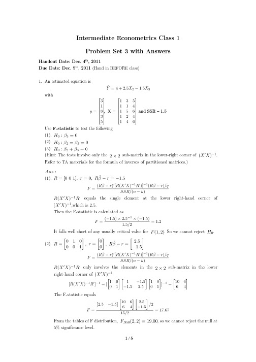
Intermediate Econometrics Class 1Problem Set 3 with AnswersHandout Date: Dec. 4th, 2011Due Date: Dec. 9th, 2011 (Hand in BEFORE class)1.An estimated equation iswith, and SSR = 1.5Use F-statistic to test the following(1).(2).(3).(Hint: The tests involve only the sub-matrix in the lower-right corner of .Refer to TA materials for the formula of inverses of partitioned matrices.)(1).equals the single element at the lower right-hand corner of,which is 2.5.Then the F-statistic is calculated asIt falls well short of any usually critical value for . So we cannot reject .(2).only involves the elements in the sub-matrix in the lowerright-hand corner ofThe F-statistic equalsFrom the tables of F distribution, , so we cannot reject the null at5% significance level.(3).Thus the test statistic becomesAgain, the test statistic falls well short of any usually critical value for . So wecannot reject .2. A four-variable regression using quarter data from 1958 to 1976 inclusive gave an estimatedequationThe explained sum of squares was 109.6, and the residual sum of squares, 18.48.(1).When the equation was re-estimated with three seasonal dummies added to thespecification, the explained sum of squares rose to 114.8. Test for the presence of seasonality.To test for the presence of seasonality we test the joint significance of the three seasonal dummy variables. The restricted is 18.48, while the unrestricted isThe rule-of-thumb F-statistic is calculated asThe 5% critical value is (is usually not given in statistic tables,so here we use the instead). We can reject the hypothesis of no seasonality at 5%significance level.(2).Two further regressions based on the original specification were run for the sub-periods1958.1 to 1968.4 and 1969.1 to 1976.4, yielding residual sums of squares of 9.32 and 7.46, respectively. Test for the constancy of the relationship over the two sub-periods.To test the parameter consistency over the two sub-samples, consider the Chow test,The 5% critical value is . Hence we cannot reject the hypothesis ofparameter constancy at 5% significance level.3.Survey records for a large sample of families show the following weekly consumptionexpenditure (Y) and weekly income (X):Y 70 76 91 …… 120 146 135 X 80 95 105 …… 155 165 175* * *Families with an asterisk (*) reported that their income is higher than in the previous year.(1).To examine the impact of weekly income on weekly consumptions, one sets up thefollowing modelHe is concerned that the error terms may have heterogeneous variance. Derive the robust standard error of .Under HSK, the large sample distribution of isThe sample estimate of iswhereThe robust standard error of is the 2nd diagonal element of the estimated covariancematrix of(2).If he wants to estimate directly the elasticity of consumption with respect of income, howshould he modify the model in (1).(3).If he wants to test whether the event of an increase in income, holding the level of incomeunchanged, helps to explain the consumption behavior, how should he extend the model in (1)?(4).If he wants to test whether the marginal propensity to consume (the slope coefficient) offamilies experiencing an increase in income is different from that of families who did not experience an increase, how should he extend the model in (3)?4.Consider the equationwhere is the cumulative college grade point average, is size of high schoolgraduating class, in hundreds, is academic percentile in graduating class, iscombined SAT score, is a dummy gender variable, and is a dummy variablewhich is one for student-athletes.(1).What are your expected signs for the coefficients in this equation? Explain.Holding all other variables constant, the expected sign for high school size should be negative, but at a diminishing rate, because larger high schools tend to have lower teacher-to-student ratios, and the effect becomes less important as the size increase. The higher sat should be positively related to GPA. So should hsperc and female (why should this be the case might be controversial; either because female students tend to study harder to overcome gender discrimination in society, or they tend to take classes where they excel more). I suppose the coefficient for athlete might be negative. However, this might just be my own prejudice.(This answer is provided by the solution manual of Introductory Econometrics: A Modern Approach. It is only for your reference. You’ll receive full credit so long your arguments make sense.)(2).To allow the effect of being an athlete to differ by gender, how should you extend themodel? Write out the null hypothesis if you want to test whether there is no ceteris paribus difference between women athletes and women nonalthletes.Adding to the model we have:In this setup, the intercepts for 4 different categories are:Male non-athleteMale athleteFemale non-athleteFemale athleteSo the test between female athletes and female non-athletes is the test of5.One application of ADL models is the Adaptive Expectation Model:⁄(5.1)⁄(5.2)wheredemand for moneyinterest rate (observables)equilibrium, optimum, or expected long-run interest rate (unobservable)the coefficient of expectation (,)Rewrite Eq.(5.2)⁄(5.3)Substitute Eq. (5.3) into Eq. (5.2)⁄(5.4)(1).Lag Eq. (5.1) one period, then substitute it into Eq. (5.4). You should be able to show thatthe short-run demand is in essence an ADL process of the observables. Write outthe model, and calculate the long-run impact multiplier of .The ADL model isUse lag operator to rewrite the modelThe long-run impact multiplier of isNote the long-run impact multiplier of in the short-rum model is essentially the coefficientof in Eq. (5.1), the equilibrium/long-run model.(2).Now consider another application that incorporates the partial adjustment of into theAdoptive Expectations Model:where are defined as in (1), and:actual capital stock (observable)desired level of capital (unobservable)the coefficient of adjustmentShow that the observed short-run demand is in essence an ADL process. (Hint: Ifyou derive the model correctly, you will find the error terms are serially correlated.)The ADL model is。
以往《计量经济学》作业答案(2)
以往计量经济学作业答案第一次作业:1-2. 计量经济学旳研究旳对象和内容是什么?计量经济学模型研究旳经济关系有哪两个基本特性?答:计量经济学旳研究对象是经济现象,是研究经济现象中旳具体数量规律(或者说,计量经济学是运用数学措施,根据记录测定旳经济数据,对反映经济现象本质旳经济数量关系进行研究)。
计量经济学旳内容大体涉及两个方面:一是措施论,即计量经济学措施或理论计量经济学;二是应用,即应用计量经济学;无论是理论计量经济学还是应用计量经济学,都涉及理论、措施和数据三种要素。
计量经济学模型研究旳经济关系有两个基本特性:一是随机关系;二是因果关系。
1-4.建立与应用计量经济学模型旳重要环节有哪些?答:建立与应用计量经济学模型旳重要环节如下:(1)设定理论模型,涉及选择模型所涉及旳变量,拟定变量之间旳数学关系和拟定模型中待估参数旳数值范畴;(2)收集样本数据,要考虑样本数据旳完整性、精确性、可比性和一致性;(3)估计模型参数;(4)模型检查,涉及经济意义检查、记录检查、计量经济学检查和模型预测检查。
1-6.模型旳检查涉及几种方面?其具体含义是什么?答:模型旳检查重要涉及:经济意义检查、记录检查、计量经济学检查、模型预测检查。
在经济意义检查中,需要检查模型与否符合经济意义,检查求得旳参数估计值旳符号与大小与否与根据人们旳经验和经济理论所拟订旳盼望值相符合;在记录检查中,需要检查模型参数估计值旳可靠性,即检查模型旳记录学性质;在计量经济学检查中,需要检查模型旳计量经济学性质,涉及随机扰动项旳序列有关检查、异方差性检查、解释变量旳多重共线性检查等;模型预测检查重要检查模型参数估计量旳稳定性以及对样本容量变化时旳敏捷度,以拟定所建立旳模型与否可以用于样本观测值以外旳范畴。
第二次作业:2-1答:P27 6条2-3 线性回归模型有哪些基本假设?违背基本假设旳计量经济学模型与否就不可估计?答:(1)略(2)违背基本假设旳计量经济学模型还是可以估计旳,只是不能使用一般最小二乘法进行估计。
计量经济学第3章习题作业
A n ≥ k +1 B n ≤ k +1 C n ≥ 30 D n ≥ 3(k +1)
6. 对于 Yi =βˆ0 + βˆ1Xi +ei ,以σˆ 表示估计标准误差,r 表示相关系数,则有( ) A σˆ=0时,r=1
B σˆ=0时,r=-1
C σˆ=0时,r=0
7. 简述变量显著性检验的步骤。 8. 简述样本相关系数的性质。 9. 试述判定系数的性质。
五、综合题
1. 为了研究深圳市地方预算内财政收入与国内生产总值的关系,得到以下数据:
年份
地方预算内财政收入 Y
国内生产总值(GDP)X
(亿元)
(亿元)
1990
21.7037
171.6665
1991
27.3291
184.7908
1436.0267
2000
225.0212
1665.4652
2001
265.6532
1954.6539
要求:
(1)建立深圳地方预算内财政收入对 GDP 的回归模型;
(2)估计所建立模型的参数,解释斜率系数的经济意义;
(3)对回归结果进行检验;
(4)若是 2005 年的国内生产总值为 3600 亿元,确定 2005 年财政收入的预测值和预
)
A 可靠性
B 合理性
C 线性
D 无偏性
E 有效性
5. 剩余变差是指(
)
A 随机因素影响所引起的被解释变量的变差
B 解释变量变动所引起的被解释变量的变差
C 被解释变量的变差中,回归方程不能做出解释的部分
D 被解释变量的总变差与回归平方和之差
计量经济学-课后作业-全部

第一次作业1.下列假想模型是否属于揭示因果关系的计量经济学模型?为什么?⑴ 其中为第年农村居民储蓄增加额(亿元)、为第年城镇S R t t =+1120012..S t t R t t 居民可支配收入总额(亿元)。
⑵其中为第()年底农村居民储蓄余额(亿元)、S R t t -=+144320030..S t -11-t 为第年农村居民纯收入总额(亿元)。
R t t 2.指出下列假想模型中的错误,并说明理由: (1)RS RI IV t t t =-+83000024112...其中,为第年社会消费品零售总额(亿元),为第年居民收入总额(亿元)(城RS t t RI t t 镇居民可支配收入总额与农村居民纯收入总额之和),为第年全社会固定资产投资总IV t t 额(亿元)。
(2)tt Y C 2.1180+=其中, 、分别是城镇居民消费支出和可支配收入。
C Y (3)tt t L K Y ln 28.0ln 62.115.1ln -+=其中,、、分别是工业总产值、工业生产资金和职工人数。
Y K L 3.下列假想的计量经济模型是否合理,为什么? (1)εβα++=∑i GDP GDP i其中,是第产业的国内生产总值。
)3,2,1(GDP i =i i (2)εβα++=21S S 其中, 、分别为农村居民和城镇居民年末储蓄存款余额。
1S 2S (3)εββα+++=t t t L I Y 21其中,、、分别为建筑业产值、建筑业固定资产投资和职工人数。
Y I L(4)εβα++=t t P Y 其中,、分别为居民耐用消费品支出和耐用消费品物价指数。
Y P (5)ε+=)(财政支出财政收入f (6)ε+=),,,(21X X K L f 煤炭产量其中,、分别为煤炭工业职工人数和固定资产值,、分别为发电量和钢铁产量。
L K 1X 2X 第二次作业学软件(建议使用Eviews6.0)完成建立计量经济学模型的全过程,通过练习,能够熟练应用计量经济学软件Eviews6.0中的最小二乘法(上机操作)。
金融计量经济学第三次作业

金融计量经济学第三次作业陈实 12000158011、 解答:在模型两边同时除以inc 可得,01234//////inc Beer inc inc price inc educ inc femal inc βββββε=+++++在这个式子中,误差项/u inc ε= 的方差为22[u |inc,price,educ,femal]Var()/inc Var εσ== ,即为同方差的。
2、 解答:如果模型中缺少了一个重要的自变量,WLS 不一定优于OLS 。
因为WLS 所解决的问题是异方差的问题。
而模型中缺少了一个重要的自变量则是模型设定不当的问题,WLS 并不能解决这一问题,所以也就不一定由于OLS 。
3、 解答: (1)同方差假设给出的标准差是在假设干扰项方差相同的情况下给出的,异方差稳健的标准差是在假设干扰项的方差不同的情况下给出的。
在这个例子中异方差稳健的标准差相比于同方差假设的标准差中,只有age 前的系数的标准差下降了20%,其余的标准差变化都在4%以内。
所以,在这个例子中,大多数的异方差稳健的标准差与同方差假设的标准差相近。
(2)在其他条件不变时,增加4年的教育退投资股票的概率的影响是增大:0.02940.11611.6%⨯== 的概率。
(3)·0.0200.00052Stockage age∂=-∂ ,所以当这个值小于0时,age 大于38.46,所以在39岁(含)以后,投资股票的概率会随年龄的增加而下降。
(4)虚拟变量city 的系数0.101代表的是,在其他条件相同的情况下,居住在城市的人比不居住在城市的人投资股票的概率,在期望的情况下大10.1%. (5)这个人投资股票的概率的期望值为20.6560.0069*log(2800)0.012*log(8500)0.029*160.020*470.00026*470.101*10.026*1 1.724Stock =++++-+-=这个概率大于1,在现实中是不可能的。
计量经济学课后答案——张龙版

计量经济学第一次作业第二章P858.用SPSS软件对10名同学的成绩数据进行录入,分析得r=,这说明学生的课堂练习和期终考试有密切的关系,一般平时练习成绩较高者,期终成绩也高。
9.(1)一元线性回归模型如下:Y i=ß0+ß1X i+u i其中,Yi 表示财政收入,Xi表示国民生产总值,ui为随机扰动项,ß0 ß1为待估参数。
由Eviews软件得散点图如下图:(2)Ýi=+SÊ:t:R2=0.958316 F= df=28斜率ß1=表示国民生产总值每增加1亿元,财政收入增加亿元。
(3)可决系数R2=表示在财政收入Y的总变差中由模型作出的解释部分占%,即有%由国民生产总值来解释,同时说明样本回归模型对样本数据的拟合程度较高。
R2=ESS/(ESS+RSS)ESS=RSS*R2/(1-R2)=+08)*=+08F=(n-2)ESS/RSS,ESS=F*RSS/(n-2)=*E09(4)SÊ(ß0)= SÊ(ß1)=ß1的95%的置信区间是:[ß(28)S Ê(ß1),ß1+(28)S Ê(ß1)] 代入数值得: [即:[,]同理可得,ß0的95%置信区间为[,] (5)①原假设H 0:ß0=0 备择假设:H 1:ß0≠0则ß0的t 值为:t 0=当ɑ=时t ɑ/2(28)=|t 0|=>t ɑ/2(28)= 故拒绝原假设H 0,表明模型应保留截距项。
②原假设H 0:ß1=0 备择假设:H 1:ß1≠0当ɑ=时t ɑ/2(28)= 因为|t 1|=>t ɑ/2(28)=故拒绝原假设H 0表明国民生产总值的变动对国家财政收入有显著影响.计量经济学第二次作业第二章9.(10) 、建立X 与t 的趋势模型,其回归分析结果如下:Dependent Variable: X Method: Least Squares Date: 04/19/10 Time: 22:03 Sample: 1978 2008Included observations: 31Dependent Variable: Y Method: Least Squares Date: 04/10/10 Time: 17:31 Sample: 1978 2007Included observations: 30VariableCoefficien t Std. Error t-StatisticProb.C XR-squaredMean dependent var Adjusted R-squared . dependent var . of regression Akaike info criterionSum squared resid +08 Schwarz criterionLog likelihood F-statistic Durbin-Watson statProb(F-statistic)VariableCoefficien t Std. Error t-StatisticProb.T CR-squaredMean dependent var Adjusted R-squared . dependent var . of regression Akaike info criterionSum squared resid +10 Schwarz criterionLog likelihood F-statistic Durbin-Watson statProb(F-statistic)令t=2008,其预测结果X=再根据X 对Y 进行预测,其预测结果为Y= X 2008= Y 2008=(S Ê(e 0))2—(S Ê(Y0))2=ó2 所以S Ê(e 0)= 在95%的置信度下,Y 2008的预测区间为: [Y 0-t α/2S Ê(e 0),Y 0+t α/2S Ê(e 0)]=[,]第三章P124,6. 该家庭在衣着用品方面的开支(Y )对总开支(X 1)以及衣着用品价格(X 2)的最小二乘估计结果如下:Dependent Variable: Y Method: Least Squares Date: 04/20/10 Time: 09:24 Sample: 1991 2000Included observations: 10VariableCoefficien t Std. Error t-StatisticProb.C X1 X2R-squaredMean dependent var Adjusted R-squared . dependent var . of regression Akaike info criterionSum squared resid Schwarz criterion Log likelihoodF-statisticDurbin-Watson stat Prob(F-statistic)12- 3.755455 + 0.183866 + 0.301746 i i i Y X X = :SE (2.679575) (0.028973) (0.167644) :t (-1.401511) (6.346071) (1.799923) :P (0.2038) (0.0004) (0.1149) 20.960616R = 2 0.949364R = :F (85.36888) ():(0.000012)P F :(2.725104)DW 7df =在=5%α的显著性水平下,对解释变量的估计参数1ˆβ、2ˆβ进行检验: 0111:0,:0H H ββ=≠,1{ 6.346071}0.0004<=0.05P t t α>==,1t 落入拒绝域,接受备择假设1H ,1ˆβ不显著为0,即就单独而言,总开支(X 1)对衣着用品方面的开支(Y )影响显著。
- 1、下载文档前请自行甄别文档内容的完整性,平台不提供额外的编辑、内容补充、找答案等附加服务。
- 2、"仅部分预览"的文档,不可在线预览部分如存在完整性等问题,可反馈申请退款(可完整预览的文档不适用该条件!)。
- 3、如文档侵犯您的权益,请联系客服反馈,我们会尽快为您处理(人工客服工作时间:9:00-18:30)。
点击主界面菜单Quick\Estimate Equation,在弹出的对话框中输入Y、C、X,操作如下图:
(2) a.生成残差序列。
在工作文件中点击Object'Generate Series ,在
弹出的窗口中,在主窗口键入命令如下“e1=resid A2 ”得到残差平方和序
列e10如下图:
b.绘制el与x的散点图。
按住Ctrl键,同时选择变量X与e2以组对象方式打幵,进入数据列表,再点击View\Graph\Scatter\Simple Scatter , 可得散点图。
如上图:
(3)a.设定一元线性回归模型为:
点击主界面菜单Quick'Estimate Equatio n ,在弹出的对话框中输入Iog(e1)、C X,得出结果如下图:
b.在工作文件中点击Object'Generate Series ,在弹出的窗口中,在主窗口键入命令如下”w=1/sqr(exp+*x)) ”得出权数W.
c.点击主界面菜单Quick'Estimate Equation,在弹出的Specification 对话框中输入Y、C、X,在Options中的Weight series中填入权数w.如下图:
(1)结果
Depe ndent Variable: Y
Method: Least Squares
Date: 12/5/16 Time: 19:57
Sample: 1 20
In cluded observatio ns: 20
Coeffici Std. t-Statist
Variable ent Error ic Prob.
F=
估计结果显示,即使在10%的显着性水平下,都不拒绝常数项为零的假设。
(2) 由b 的图可知,残差平方e1与x 大致存在递增关系,即存在单调增型 异方差。
(3) 通过加权得出的方程结果如下:
Method: Least Squares
Date: 12/5/16 Time: 20:01 Sample: 1 20
X
R-squared Adjusted R-squared
.of regressi on Sum squared resid
Log likelihood F-statistic Prob(F-statisti c)
得到模型的估计结果为:
Mean depe ndent var
.dependent var Akaike info
criterio n
Schwarz criteri on Hannan-Qu inn
criter.
Durb in-Wats on stat
In eluded observatio ns: 20
Weight ing series: W
Weight type: Stan dard deviatio n (average scali ng) HAC sta ndard errors & covaria nee (Bartlett kernel, Newey-West fixed
ban dwidth =
Hannan-Qu inn
Log likelihood criter.
F-statistic Durb in-Wats on stat Prob(F-statisti
c) Weighted mean dep. Wald Prob(Wald
F-statistic F-statistic)
Un weighted
Statistics
R-squared Mean depe ndent var Adjusted
R-squared .dependent var
.of regressi on Sum squared resid Durbi n-Wats on
stat
得到模型的估计结果为:
F=。