曲线拟合——最小二乘法算法
第六章_曲线拟合的最小二乘法

25
24
o
1 2 3 4 5 6 7 8
t
(0 , 0 ) (0 , 1 ) a0 (0 , f ) ( , ) ( , ) a ( , f ) 1 1 1 1 1 0
计算系数
(0 , 0 ) 1 8
bt y
则矛盾方程组为:
1 1 1 1 1 0.669131 0.370370 0.390731 0.500000 a 0.621118 0.121869 b 0.309017 0.833333 0.980392 0.587785
例1. 对彗星1968Tentax的移动在某极坐标系下有如 下表所示的观察数据,假设忽略来自行星的干扰,坐 r 标应满足: 1 e p 其中:p为参数,e为偏心率, cos
试用最小二乘法拟合p和e。
r
2.70 480
2.00 670
1.61 830
1.20 1080
1.02 1260
得正则方程组为:
5.0 0.284929 0.284929 a 3.305214 b 0.314887 1.056242
解得: a 0.688617
b 0.483880
1 则: p 1.452186 e bp 0.702684 a 1.452186 则拟合方程为: r 1 0.702684 cos
第六章 曲线拟合的最小二乘法
§6.1 引言
§6.2 线性代数方程组的最小二乘解
§6.3 曲线最小二乘拟合
§1 引言
如果实际问题要求解在[a,b]区间的每一点都 “很好地” 逼近f(x)的话,运用插值函数有时就要 失败。另外,插值所需的数据往往来源于观察测量, 本身有一定的误差。要求插值曲线通过这些本身有误 差的点,势必使插值结果更加不准确。 如果由试验提供的数据量比较大,又必然使得插 值多项式的次数过高而效果不理想。 从给定的一组试验数据出发,寻求函数的一个近 似表达式y=(x),要求近似表达式能够反映数据的基 本趋势而又不一定过全部的点(xi,yi),这就是曲线拟 合问题,函数的近似表达式y=(x)称为拟合曲线。本 章介绍用最小二乘法求拟合曲线。
计算方法 第三章曲线拟合的最小二乘法20191103

§2 多项式拟合函数
例3.1 根据如下离散数据拟合曲线并估计误差
x 1 23 4 6 7 8 y 2 36 7 5 3 2
解: step1: 描点
7
*
step2: 从图形可以看出拟
6 5
*
合曲线为一条抛物线:
4
y c0 c1 x c2 x2
3 2 1
* *
* * *
step3: 根据基函数给出法
法
18
定理 法方程的解是存在且唯一的。
证: 法方程组的系数矩阵为
(0 ,0 ) (1 ,0 )
G
(0
,1
)
(1 ,1 )
(0 ,n ) (1 ,n )
(n ,0 )
(
n
,
1
)
(n ,n )
因为0( x),1( x), ...,n( x)在[a, b]上线性无关,
所以 G 0,故法方程 GC F 的解存在且唯一。
第三章 曲线拟合的最小二乘法
2
最小二乘拟合曲线
第三章 曲线拟合的最小二乘
2021/6/21
法
3
三次样条函数插值曲线
第三章 曲线拟合的最小二乘
2021/6/21
法
4
Lagrange插值曲线
第三章 曲线拟合的最小二乘
2021/6/21
法
5
一、数据拟合的最小二乘法的思想
已知离散数据: ( xi , yi ), i=0,1,2,…,m ,假设我们用函
便得到最小二乘拟合曲线
n
* ( x) a*j j ( x) j0
为了便于求解,我们再对法方程组的导出作进一步分析。
第三章 曲线拟合的最小二乘
曲线拟合的最小二乘法实验
Lab04.曲线拟合的最小二乘法实验【实验目的和要求】1.让学生体验曲线拟合的最小二乘法,加深对曲线拟合的最小二乘法的理解;2.掌握函数ployfit和函数lsqcurvefit功能和使用方法,分别用这两个函数进行多项式拟合和非多项式拟合。
【实验内容】1.在Matlab命令窗口,用help命令查询函数polyfit和函数lsqcurvefit 功能和使用方法。
2.用多项式y=x3-6x2+5x-3,产生一组数据(xi,yi)(i=1,2,…,n),再在yi上添加随机干扰(可用rand产生(0,1)均匀分布随机数,或用randn产生N(0,1)均匀分布随机数),然后对xi和添加了随机干扰的yi用Matlab提供的函数ployfit用3次多项式拟合,将结果与原系数比较。
再作2或4次多项式拟合,分析所得结果。
3.用电压V=10伏的电池给电容器充电,电容器上t时刻的电压为,其中V0是电容器的初始电压,τ是充电常数。
对于下面的一组t,v数据,用Matlab提供的函数lsqcurvefit确定V0和τ。
t(秒) 0.5 1 2 3 4 5 7 9v(伏) 6.36 6.48 7.26 8.22 8.66 8.99 9.43 9.63 【实验仪器与软件】1.CPU主频在1GHz以上,内存在128Mb以上的PC;2.Matlab 6.0及以上版本。
实验讲评:实验成绩:评阅教师:200 年月日问题及算法分析:1、利用help命令,在MATLAB中查找polyfit和lsqcurvefit函数的用法。
2、在一组数据(xi,yi)(i=1,2,…,n)上,对yi上添加随机干扰,运用多项式拟合函数,对数据进行拟合(分别用2次,3次,4次拟合),分析拟合的效果。
3、根据t和V的关系画散点图,再根据给定的函数运用最小二乘拟合函数,确定其相应参数。
第一题:(1)>> help polyfitPOLYFIT Fit polynomial to data.P = POLYFIT(X,Y,N) finds the coefficients of a polynomial P(X) ofdegree N that fits the data Y best in a least-squares sense. P is arow vector of length N+1 containing the polynomial coefficients indescending powers, P(1)*X^N + P(2)*X^(N-1) +...+ P(N)*X + P(N+1).[P,S] = POLYFIT(X,Y,N) returns the polynomial coefficients P and astructure S for use with POLYVAL to obtain error estimates forpredictions. S contains fields for the triangular factor (R) from a QRdecomposition of the Vandermonde matrix of X, the degrees of freedom(df), and the norm of the residuals (normr). If the data Y are random,an estimate of the covariance matrix of P is(Rinv*Rinv')*normr^2/df,where Rinv is the inverse of R.[P,S,MU] = POLYFIT(X,Y,N) finds the coefficients of a polynomial inXHAT = (X-MU(1))/MU(2) where MU(1) = MEAN(X) and MU(2) = STD(X). Thiscentering and scaling transformation improves the numerical propertiesof both the polynomial and the fitting algorithm.Warning messages result if N is >= length(X), if X has repeated, ornearly repeated, points, or if X might need centering and scaling.Class support for inputs X,Y:float: double, singleSee also poly, polyval, roots.Reference page in Help browserdoc polyfit>>(2)>> help lsqcurvefitLSQCURVEFIT solves non-linear least squares problems.LSQCURVEFIT attempts to solve problems of the form:min sum {(FUN(X,XDATA)-YDATA).^2} where X, XDATA, YDATA and the valuesX returned by FUN can be vectors ormatrices.X=LSQCURVEFIT(FUN,X0,XDATA,YDATA) starts at X0 and finds coefficients Xto best fit the nonlinear functions in FUN to the data YDATA (in theleast-squares sense). FUN accepts inputs X and XDATA and returns avector (or matrix) of function values F, where F is the same size asYDATA, evaluated at X and XDATA. NOTE: FUN should returnFUN(X,XDATA)and not the sum-of-squares sum((FUN(X,XDATA)-YDATA).^2).((FUN(X,XDATA)-YDATA) is squared and summed implicitly in thealgorithm.)X=LSQCURVEFIT(FUN,X0,XDATA,YDATA,LB,UB) defines a set of lower andupper bounds on the design variables, X, so that the solution is in therange LB <= X <= UB. Use empty matrices for LB and UB if no boundsexist. Set LB(i) = -Inf if X(i) is unbounded below; set UB(i) = Inf ifX(i) is unbounded above.X=LSQCURVEFIT(FUN,X0,XDATA,YDATA,LB,UB,OPTIONS) minimizes with thedefault parameters replaced by values in the structure OPTIONS, anargument created with the OPTIMSET function. See OPTIMSET for details.Used options are Display, TolX, TolFun, DerivativeCheck, Diagnostics,FunValCheck, Jacobian, JacobMult, JacobPattern, LineSearchType,LevenbergMarquardt, MaxFunEvals, MaxIter, DiffMinChange andDiffMaxChange, LargeScale, MaxPCGIter, PrecondBandWidth, TolPCG,OutputFcn, and TypicalX. Use the Jacobian option to specify that FUNalso returns a second output argument J that is the Jacobian matrix atthe point X. If FUN returns a vector F of m components when X has length n, then J is an m-by-n matrix where J(i,j) is the partialderivative of F(i) with respect to x(j). (Note that the Jacobian J isthe transpose of the gradient of F.)[X,RESNORM]=LSQCURVEFIT(FUN,X0,XDATA,YDATA,...) returns the valueof thesquared 2-norm of the residual at X: sum {(FUN(X,XDATA)-YDATA).^2}.[X,RESNORM,RESIDUAL]=LSQCURVEFIT(FUN,X0,...) returns the value of residual,FUN(X,XDATA)-YDATA, at the solution X.[X,RESNORM,RESIDUAL,EXITFLAG]=LSQCURVEFIT(FUN,X0,XDATA,YDATA,...) returnsan EXITFLAG that describes the exit condition of LSQCURVEFIT. Possiblevalues of EXITFLAG and the corresponding exit conditions are1 LSQCURVEFIT converged to a solution X.2 Change in X smaller than the specified tolerance.3 Change in the residual smaller than the specified tolerance.4 Magnitude of search direction smaller than the specified tolerance.0 Maximum number of function evaluations or of iterations reached.-1 Algorithm terminated by the output function.-2 Bounds are inconsistent.-4 Line search cannot sufficiently decrease the residual alongthecurrent search direction.[X,RESNORM,RESIDUAL,EXITFLAG,OUTPUT]=LSQCURVEFIT(FUN,X0,XDATA,YDATA ,...)returns a structure OUTPUT with the number of iterations taken inOUTPUT.iterations, the number of function evaluations inOUTPUT.funcCount,the algorithm used in OUTPUT.algorithm, the number of CG iterations (ifused) in OUTPUT.cgiterations, the first-order optimality (if used)inOUTPUT.firstorderopt, and the exit message in OUTPUT.message.[X,RESNORM,RESIDUAL,EXITFLAG,OUTPUT,LAMBDA]=LSQCURVEFIT(FUN,X0,XDAT A,YDATA,...)returns the set of Lagrangian multipliers, LAMBDA, at the solution:LAMBDA.lower for LB and LAMBDA.upper for UB.[X,RESNORM,RESIDUAL,EXITFLAG,OUTPUT,LAMBDA,JACOBIAN]=LSQCURVEFIT(FU N,X0,XDATA,YDATA,...)returns the Jacobian of FUN at X.ExamplesFUN can be specified using @:xdata = [5;4;6]; % example xdataydata = 3*sin([5;4;6])+6; % example ydatax = lsqcurvefit(@myfun, [2 7], xdata, ydata)where myfun is a MATLAB function such as:function F = myfun(x,xdata)F = x(1)*sin(xdata)+x(2);FUN can also be an anonymous function:x = lsqcurvefit(@(x,xdata) x(1)*sin(xdata)+x(2),[2 7],xdata,ydata)If FUN is parameterized, you can use anonymous functions to capture theproblem-dependent parameters. Suppose you want to solve the curve-fittingproblem given in the function myfun, which is parameterized by its secondargument c. Here myfun is an M-file function such asfunction F = myfun(x,xdata,c)F = x(1)*exp(c*xdata)+x(2);To solve the curve-fitting problem for a specific value of c, first assignthe value to c. Then create a two-argument anonymous function that capturesthat value of c and calls myfun with three arguments. Finally, pass thisanonymous function to LSQCURVEFIT:xdata = [3; 1; 4]; % example xdataydata = 6*exp(-1.5*xdata)+3; % example ydatac = -1.5; % define parameterx = lsqcurvefit(@(x,xdata) myfun(x,xdata,c),[5;1],xdata,ydata) See also optimset, lsqnonlin, fsolve, @, inline.Reference page in Help browserdoc lsqcurvefit>>第二题:1 三次线性拟合clear allx=0:0.5:5;y=x.^3-6*x.^2+5*x-3;y1=y;for i=1:length(y)y1(i)=y1(i)+rand;enda=polyfit(x,y1,3);b=polyval(a,x);plot(x,y,'*',x,b),aa =1.0121 -6.1033 5.1933 -2.4782② 二次线性拟合clear allx=0:0.5:20;y=x.^3-6*x.^2+5*x-3;y1=y;for i=1:length(y)y1(i)=y1(i)+rand;enda=polyfit(x,y1,2);b=polyval(a,x);plot(x,y,'*',x,b),aa =23.9982 -232.0179 367.9756③ 四次线性拟合clear allx=0:0.5:20;y=x.^3-6*x.^2+5*x-3;y1=y;for j=1:length(y)y1(j)=y1(j)+rand;enda=polyfit(x,y1,4);b=polyval(a,x);plot(x,y,'*',x,b),aa =-0.0001 1.0038 -6.0561 5.2890 -2.8249 >>第三题:1 拟合曲线为:f(x)=定义函数:function f=fun(a,x)f=a(1)-(a(1)-a(2))*exp(-a(3)*x);主程序:clear allclcx=[0.5 1 2 3 4 5 7 9];y=[6.36 6.48 7.26 8.22 8.66 8.99 9.43 9.63];a0=[1 1 1];a=lsqcurvefit('fun',a0,x,y);y1=a(1)-(a(1)-a(2))*exp(-a(3)*x);plot(x,y,'r*',x,y1,'b')V1=a(2)tei=1/a(3)Optimization terminated: relative function value changing by less than OPTIONS.TolFun.。
计算方法(3)-曲线拟合的最小二乘法

m
m
使 Wi [ * (xi ) i 1
yi ]2
min ( x)
Wi [ (xi )
i 1
yi ]2
其 中 (x) a0 0 (x) a11 (x) an n (x)是
中 任 一 函 数;Wi (i 1, , m)是 一 列 正 数, 称 为 权.
第三章 曲线拟合的最小二乘法
§1 引言 §2 最小二乘法 §3 最小二乘法的求法 §4 加权最小二乘法
*§5 利用正交函数作最小二乘拟合
1
§1 引言
一.曲线拟合问题
从一组实验数据(xi , yi )(i 1,2, , m)出发,
寻求函数y (x)的一个近似表达式
m
xin
i1
m
xi
i 1 m
xi2
i 1
m
x n1 i
i 1
m
xin
i 1 m
xn1 i
i 1
m
xi2n
a0 a1 an
m
WI xin
i 1
m
Wi xin1
i 1
m
Wi xi2n
a0 a1 an
m
Wi yi
i 1 m
Wi xi yi
i 1
m
Wi xin yi
是中 任 一 函 数
5
§3 最小二乘解的求法
一.法方程组
最小二乘解 * (x) a0* 0 (x) a1*1 (x) an* n (x)
曲线拟合的最小二乘法

由 ln y ln a bx ,可以先做 y* a* bx
可以先做出 ln y 的一次线性拟合
例2 设一发射源强度公式为
观测数据如下
I
I
eat
0
ti 0.2 0.3 0.4 0.5 0.6 0.7 0.8 Ii 3.16 2.38 1.75 1.34 1.00 0.74 0.56
2.9611
a b
2.31254 0.0870912
(1)、y ax2 b
解:函数空间的基
x2 ,1 ,然后列出法方程
x2, x2 D 1, x2 D
1, x2 D
1,1D
a b
f
, f
x2 D
,1D
370
34
34
5
a b
3.5a1 1.9891 2.03a1 0.1858
aa1012.7.839
ea0 =5.64 a=-2.89
则 I=5.64e-2.89t
3.2.3 最小二乘法一般形式
span{0,1,n} 0 ,1,n 为线性无关的基函数
(x) a00 (x) ann (x)
i 1
n
( y, j ) ik xi j xi j=0,1,2,…,m i 1
则法方程组可写成以下形式
0 1
,0 ,0
m ,0
0 ,1 1,1
m ,1
第5章-1 曲线拟合(线性最小二乘法)讲解
求所需系数,得到方程: 29.139a+17.9b=29.7076 17.9a+11b=18.25
通过全选主元高斯消去求得:
a=0.912605
b=0.174034
所以线性拟合曲线函数为: y=0.912605x+0.174034
练习2
根据下列数据求拟合曲线函数: y=ax2+b
x 19 25 31 38 44 y 19.0 32.3 49.0 73.3 97.8
∑xi4 a + ∑xi2 b = ∑xi 2yi
∑xi2 a + n b = ∑yi
7277699a+5327b=369321.5 5327a+5b=271.4
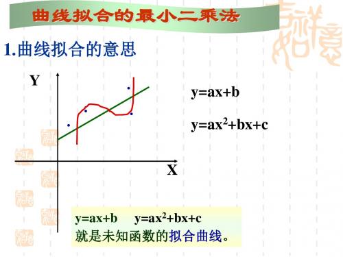
曲线拟合的最小二乘法
1.曲线拟合的意思
Y
.
.
.
.
y=ax+b y=ax2+bx+c
X
y=ax+b y=ax2+bx+c 就是未知函数的拟合曲线。
2最小二乘法原理
观测值与拟合曲线值误差的平方和为最小。
yi y0 y1 y2 y3 y4…… 观测值 y^i y^0 y^1 y^2 y^3 y^4…… 拟合曲线值
拟合曲线为: y=(-11x2-117x+56)/84
x
yHale Waihona Puke 1.61 1.641.63 1.66
1.6 1.63
1.67 1.7
1.64 1.67
1.63 1.66
1.61 1.64
1.66 1.69
1.59 1.62
曲线拟合的最小二乘法
§7 曲线拟合的最小二乘法7-1 一般的最小二乘逼近(曲线拟合的最小二乘法)最小二乘法的一般提法是:对给定的一组数据(,)(0,1,,)i i x y i m =L ,要求在函数类01{,,,}n ϕϕϕϕ=L 中找一个函数*()y S x =,使误差平方和22*222()001[()]min [()]m m m i i i i iS x i i i S x y S x y ϕδδ∈=====−=−∑∑∑其中 0011()()()()()n n S x a x a x a x n m ϕϕϕ=+++<L 带权的最小二乘法: 2220()[()()]mi i i i x S x f x δω==−∑其中()0x ω≥是[a,b ]上的权函数。
用最小二乘法求曲线拟合的问题,就是在()S x 中求一函数*()y S x =,使22δ取的最小。
它转化为求多元函数20100(,,,)()[()()]m n n i j j i i i j I a a a x a x f x ωϕ===−∑∑L 的极小点***01(,,,)n a a a L 问题。
由求多元函数极值的必要条件,有002()[()()]()0m n i j j i i k i i j k I x a x f x x a ωϕϕ==∂=−=∂∑∑ ),,1,0(n k L =若记 0(,)()()()m j k ij i k i i x x x ϕϕωϕϕ==∑ 0(,)()()()mk i i k i k i f x f x x d ϕωϕ==≡∑ ),,1,0(n k L = 则上式可改写为0(,)n kj j k j a d ϕϕ==∑ ),,1,0(n k L =这个方程称为法方程,矩阵形式.Ga d =其中 0101(,,,),(,,,)T T n n a a a a d d d d ==L L ,0001010111011(,)(,)(,)(,)(,)(,)(,)(,)(,)n n n n n n G ϕϕϕϕϕϕϕϕϕϕϕϕϕϕϕϕϕϕ− = LL L L L L L 由于01,,,n ϕϕϕL 线性无关,故0G ≠,方程组存在唯一解*(0,1,,),k k a a k n ==L从而得到函数()f x 的最小二乘解为****0011()()()()n n S x a x a x a x ϕϕϕ=+++L 可证 *2200()[()()]()[()()]m mii i i i i i i x S x f x x S x f x ωω==−≤−∑∑ 故*()S x 使所求最小二乘解。
数值分析论文--曲线拟合的最小二乘法
---------------------------------------------------------------最新资料推荐------------------------------------------------------ 数值分析论文--曲线拟合的最小二乘法曲线拟合的最小二乘法姓名:徐志超学号:2019730059 专业:材料工程学院:材料科学与工程学院科目:数值分析曲线拟合的最小二乘法一、目的和意义在物理实验中经常要观测两个有函数关系的物理量。
根据两个量的许多组观测数据来确定它们的函数曲线,这就是实验数据处理中的曲线拟合问题。
这类问题通常有两种情况:一种是两个观测量 x 与 y 之间的函数形式已知,但一些参数未知,需要确定未知参数的最佳估计值;另一种是 x 与 y 之间的函数形式还不知道,需要找出它们之间的经验公式。
后一种情况常假设 x 与 y 之间的关系是一个待定的多项式,多项式系数就是待定的未知参数,从而可采用类似于前一种情况的处理方法。
在两个观测量中,往往总有一个量精度比另一个高得多,为简单起见把精度较高的观测量看作没有误差,并把这个观测量选作x,而把所有的误差只认为是y 的误差。
设 x 和 y 的函数关系由理论公式 y=f(x; c1, c2, cm)1 / 13(0-0-1)给出,其中 c1, c2, cm 是 m 个要通过实验确定的参数。
对于每组观测数据(xi, yi) i=1, 2,, N。
都对应于 xy 平面上一个点。
若不存在测量误差,则这些数据点都准确落在理论曲线上。
只要选取m 组测量值代入式(0-0-1),便得到方程组yi=f (x;c1,c2,cm)(0-0-2)式中 i=1,2,, m.求 m 个方程的联立解即得 m 个参数的数值。
显然Nm 时,参数不能确定。
在 Nm 的情况下,式(0-0-2)成为矛盾方程组,不能直接用解方程的方法求得 m 个参数值,只能用曲线拟合的方法来处理。
excel拟合曲线用的最小二乘法
Excel拟合曲线用的最小二乘法1. 介绍Excel作为一款常用的办公软件,被广泛应用于数据分析和处理,而拟合曲线是数据分析中常用的方法之一。
拟合曲线用的最小二乘法是一种常见的拟合方法,通过最小化数据点与拟合曲线之间的距离来找到最佳拟合曲线,从而对数据进行预测和分析。
在本文中,我将从深度和广度的角度来探讨Excel拟合曲线用的最小二乘法,带你深入探索这一主题。
2. 最小二乘法的原理在Excel中进行曲线拟合时,最小二乘法是一种常用的拟合方法。
其原理是通过最小化残差平方和来找到最佳拟合曲线。
残差是指每个数据点到拟合曲线的垂直距离,最小二乘法通过调整拟合曲线的参数,使得残差平方和最小化,从而得到最佳拟合曲线。
在Excel中,可以利用内置函数或插件来实现最小二乘法的曲线拟合,对于不同类型的曲线拟合,可以选择不同的拟合函数进行拟合。
3. Excel中的拟合曲线在Excel中进行拟合曲线时,首先需要将数据导入Excel,然后利用内置的数据分析工具或者插件来进行曲线拟合。
通过选择拟合函数、调整参数等操作,可以得到拟合曲线的相关信息,如拟合优度、参数估计值等。
可以根据拟合曲线的结果来对数据进行预测和分析,从而得到对应的结论和见解。
4. 个人观点与理解对于Excel拟合曲线用的最小二乘法,我认为这是一种简单而有效的数据分析方法。
它能够快速对数据进行拟合,并得到拟合曲线的相关信息,对于数据的预测和分析具有一定的帮助。
然而,也需要注意到拟合曲线并不一定能够准确描述数据的真实情况,需要结合实际背景和专业知识进行分析和判断。
在使用最小二乘法进行曲线拟合时,需要注意数据的可靠性和拟合结果的可信度,以避免出现不准确的结论和偏差的情况。
5. 总结通过本文的探讨,我们对Excel拟合曲线用的最小二乘法有了更深入的了解。
最小二乘法的原理、Excel中的实际操作以及个人观点与理解都得到了充分的展示和探讨。
在实际应用中,需要结合具体情况和专业知识来灵活运用最小二乘法进行曲线拟合,从而得到准确的分析和预测结果。
曲线最小二乘法拟合
最小二乘法拟合曲线算法1、概述给定数据点P(x i ,y i ),其中i=1,2,…,n 。
求近似曲线y= φ(x)。
并且使得近似曲线与y=f(x)的偏差最小。
近似曲线在点pi 处的偏差δi = φ(x i )-y ,i=1,2,...,n 。
按偏差平方和最小的原则选取拟合曲线,这种方法为最小二乘法,偏差平方和公式为:min σ2 = (φ(x i −y i ))2ni =1n i =12、推导过程1)设拟合多项式为:y = a 0+ a 1x +⋯+a k x k2)各点到这条曲线的距离之和,即偏差平方如下:R 2= [y i −(a 0+ a 1x +⋯+a k x k )]2ni =13)多项式系数为学习对象,为了求得符合条件的系数值,对上面等式的a i 分别求导,得:−2 y i − a 0+ a 1x +⋯+a k x k =0ni=1−2 y i − a 0+ a 1x +⋯+a k x k x =0ni=1……−2 y i − a 0+ a 1x +⋯+a k x k x k =0ni=14)将等式移项化简,得:a 0+ a 1x +⋯+a k x k = y i ni =1n i =1a 0+ a 1x +⋯+a k x k x = y i x ni =1n i =1……a 0+ a 1x +⋯+a k x k x k = y i x k ni =1n i =15)依上式得矩阵为:x i0 ni=1⋯x i kni=1⋮⋱⋮x i k ni=1⋯x i2kni=1a0⋮a k=y i x i0ni=1⋮y i x i kni=1上边等式左边为1+K阶对称矩阵,解此矩阵方程即可得到曲线系数a k6)对于AX=B,A为对称矩阵,对称矩阵可以分解为一个下三角矩阵、一个上三角矩阵(下三角矩阵的转置)和一个对角线矩阵相乘。
即A=LDL T所以AX=LDL T X=B,令DL T X=Y -> LY=B,其中L为下三角矩阵,且已知,可求出Y。
- 1、下载文档前请自行甄别文档内容的完整性,平台不提供额外的编辑、内容补充、找答案等附加服务。
- 2、"仅部分预览"的文档,不可在线预览部分如存在完整性等问题,可反馈申请退款(可完整预览的文档不适用该条件!)。
- 3、如文档侵犯您的权益,请联系客服反馈,我们会尽快为您处理(人工客服工作时间:9:00-18:30)。
曲线拟合——最小二乘法算法
一、目的和要求
1)了解最小二乘法的基本原理,熟悉最小二乘算法;
2)掌握最小二乘进行曲线拟合的编程,通过程序解决实际问题。
二、实习内容
1)最小二乘进行多项式拟合的编程实现。
2)用完成的程序解决实际问题。
三、算法
1)输入数据节点数n ,拟合的多项式次数m ,循环输入各节点的数据x j , y j (j=0,1,…,n-1)
2)由x j 求S ;由x j ,y j 求T :
S k =
∑-=10n j k j x ( k=0,1,2, … 2*m ) T k = ∑-=1
0n j k j j x y ( k=0,1,2,… m )
3)由S 形成系数矩阵数组c i,j :c[i][j]=S[i+j] (i=0,1,2,…m, j=0,1,2,…,m);由T 形成系数矩阵增广部分c i,m+1:c[i][m+1]=T[i] (i=0,1,2,…m)
4)对线性方程组CA=T[或A C ],用列主元高斯消去法求解系数矩阵A=(a 0,a 1,…,a m )T
四、实验步骤
1)完成最小二乘法进行曲线拟合的程序设计及录入、编辑;
2)完成程序的编译和链接,并进行修改;
3)用书上P105例2的例子对程序进行验证,并进行修改;
4)用完成的程序求解下面的实际问题。
5)完成实验报告。
五、实验结果
1. 经编译、链接及例子验证结果正确的源程序:
#include<stdio.h>
#include<math.h>
#define Q 100
float CF(int,float);
main()
{
int i,j,n1,n,p,k,q;
float x[Q],y[Q],s[Q]={0},t[Q]={0},a[Q][Q]={0},l,sum=0;
/*以下是最小二乘的程序*/
printf("input 数据组数n");
scanf("%d",&n);
printf("input 拟合次数n1");
scanf("%d",&n1);
for(i=0;i<n;i++)
{
printf("x[%d]=",i);
scanf("%f",&x[i]);
printf("y[%d]=",i);
scanf("%f",&y[i]);
}
for(i=0;i<=2*n1;i++)
for(j=0;j<n;j++)
{
s[i]=s[i]+CF(i,x[j]);
if(i<=n1)
t[i]=t[i]+y[j]*CF(i,x[j]);
}
for(i=0;i<n1+1;i++)
for(j=0;j<n1+2;j++)
{
a[i][j]=s[i+j];
if(j==n1+1)
a[i][j]=t[i];
}
for(i=0;i<n1+1;i++)
for(j=0;j<n1+2;j++)
printf("a[%d][%d]=%f",i,j,a[i][j]); /*以下的是削去法的程序*/
for(j=0;j<=n1-1;j++)
{p=j;
for(i=j+1;i<=n1;i++)
{
if(fabs(a[j][j])<fabs(a[i][j]))
p=i;
}
if(p!=j)
for(i=j;i<=n1+1;i++)
{l=a[p][i];
a[p][i]=a[j][i];
a[j][i]=l;
}
for(k=j+1;k<=n1;k++)
{l=a[k][j]/a[j][j];
for(q=j;q<=n1+1;q++)
a[k][q]=a[k][q]-l*a[j][q];
}
}
for(i=0;i<n1+1;i++)
{for(j=0;j<n1+2;j++)
printf("a[%d][%d]=%f\n",i,j,a[i][j]);
printf("\n");}
x[n1]=a[n1][n1+1]/a[n1][n1];
for(i=n1-1;i>=0;i--)
{for(j=i+1;j<=n1;j++)
sum=a[i][j]*x[j]+sum;
x[i]=(a[i][n1+1]-sum)/a[i][i];
sum=0;
}
for(i=0;i<=n1;i++)
printf("x[%d]=%f\n",i,x[i]);
}
float CF(int i,float v)
{float a=1.0;
while(i--)a*=v;
return a;
}
2. 实例验证结果:
1)输入初始参数:
n=9,m=2
X:1 3 4 5 6 7 8 9 10
Y:10 5 4 2 1 1 2 3 4
2)结果输出:
1.实际应用
问题:
作物体运动的观测实验,得出以下实验测量数据,用最小二乘拟合求物体的运动方程。
时间t(秒) 0 0.9 1.9 3.0 3.9 5.0 距离s(cm) 0 10 30 50 80 110
解题步骤:
1)画草图
2)确定拟合方程次数为1:
用完成的程序输入数据,求取拟合方程中的未知数,得出方程:
S=-7.855.58+22.253763T
计算误差:
3)确定拟合方程次数为2:
用完成的程序输入数据,求取拟合方程中的未知数,得出方程:
S=-0.583370+11.081389T+2.248811T*T
计算误差:
六、分析和讨论
结合实际问题,进行拟合次数的分析和讨论:
七、心得(*可选)
①调试过程中遇到的问题和解决对策;②经验体会等。
以上都是我业余所写,程序肯定有很多不足之处希望大家多多指教。