桁架单元例子MATLAB 1

合集下载

桁架优化matlab算法

桁架优化matlab算法桁架优化Matlab 算法【引言】桁架是一种常见的结构体系，它由连接节点的杆件构成。

桁架通常在工程设计中用于支撑、加固或分散载荷。

优化桁架结构对于减少材料使用、提高结构强度和降低成本非常重要。

Matlab 是一种功能强大的计算软件，它提供了许多优化算法和工具。

本文将介绍如何使用Matlab 进行桁架优化的算法实现。

【第一步- 建立力学模型】桁架的力学模型是优化过程的基础。

在Matlab 中，可以使用矩阵表示力学模型。

首先，我们需要定义桁架的节点和杆件。

节点用坐标表示，杆件用节点之间的连接关系表示。

根据节点和杆件的定义，可以构建节点坐标矩阵和链接关系矩阵。

【第二步- 约束条件和目标函数】在进行桁架优化时，通常会遇到一些约束条件和目标函数。

典型的约束条件可能包括杆件的最大和最小尺寸限制、节点的最大和最小高度限制等。

目标函数可以是桁架的重量、刚度或模态频率等。

根据具体问题，我们需要定义合适的约束条件和目标函数。

【第三步- 优化算法】Matlab 提供了许多优化算法，如遗传算法、粒子群优化算法等。

我们需要选择合适的算法来解决桁架优化问题。

对于离散变量的优化，可以使用遗传算法。

对于连续变量的优化，可以使用粒子群优化算法。

选择合适的算法后，可以将约束条件和目标函数输入优化算法，得到优化结果。

【第四步- 结果分析】优化算法完成后，我们需要对结果进行分析。

可以通过绘制优化后的桁架结构来比较与原始结构的差异。

此外，还可以从目标函数的值来评估优化结果。

如果目标函数的值较小，则说明优化结果较优。

【第五步- 进一步优化】根据结果的分析，我们可以进一步优化桁架结构。

可以尝试使用不同的约束条件和目标函数，或者尝试其他优化算法。

通过多次迭代优化，逐步优化桁架结构，以得到更好的结果。

【第六步- 结论】通过以上的一步一步的回答，我们可以得出结论，桁架优化的Matlab 算法是一个有效的方法。

通过建立力学模型、定义约束条件和目标函数、选择合适的优化算法，我们可以获得优化后的桁架结构。

matlab桁架结构有限元计算

matlab桁架结构有限元计算摘要：一、引言- 介绍MATLAB在桁架结构有限元计算中的应用- 说明本文的主要内容和结构二、有限元计算原理- 有限元方法的背景和基本原理- 有限元方法在桁架结构分析中的应用三、MATLAB实现桁架结构有限元计算- MATLAB的基本操作和编程基础- 使用MATLAB进行桁架结构有限元计算的步骤和示例四、MATLAB桁架结构有限元计算的应用- 分析不同桁架结构的特点和计算结果- 探讨MATLAB在桁架结构有限元计算中的优势和局限五、结论- 总结MATLAB在桁架结构有限元计算中的应用和优势- 展望MATLAB在桁架结构分析中的未来发展方向正文：一、引言随着计算机技术的不断发展，有限元方法已经成为工程界解决复杂问题的重要手段。

MATLAB作为一款功能强大的数学软件，可以方便地实现桁架结构的有限元计算。

本文将介绍MATLAB在桁架结构有限元计算中的应用，并详细阐述其操作方法和计算原理。

二、有限元计算原理1.有限元方法的背景和基本原理有限元法是一种数值分析方法，通过将连续的求解域离散为离散的单元，将复杂的问题转化为求解单元的线性或非线性方程组。

有限元方法具有适应性强、精度高、计算效率高等优点，广泛应用于固体力学、流体力学、传热等领域。

2.有限元方法在桁架结构分析中的应用桁架结构是一种由杆件组成的结构，其节点只有三个自由度。

有限元方法可以有效地分析桁架结构的强度、刚度和稳定性，为工程设计提供理论依据。

三、MATLAB实现桁架结构有限元计算1.MATLAB的基本操作和编程基础MATLAB是一种功能强大的数学软件，可以进行矩阵运算、绘制图形、编写程序等操作。

在MATLAB中，用户可以通过编写脚本文件或使用图形界面进行各种计算和分析。

2.使用MATLAB进行桁架结构有限元计算的步骤和示例(1) 建立桁架结构模型：根据实际结构绘制桁架的节点和杆件，确定各节点的三自由度。

(2) 离散化：将桁架结构离散为有限个单元，每个单元包含若干个节点。

平面桁架结构matlab

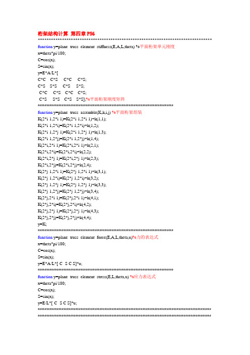
桁架结构计算第四章P56******************************************************************************* function y=plane_truss_element_stiffness(E,A,L,theta) %平面桁架单元刚度x=theta*pi/180;C=cos(x);S=sin(x);y=E*A/L*[C*C C*S -C*C -C*S;C*S S*S -C*S -S*S;-C*C -C*S C*C C*S;-C*S -S*S C*S S*S];%平面桁架刚度矩阵*******************************************************************************function y=plane_truss_assemble(K,k,i,j) %平面桁架组装K(2*i-1,2*i-1)=K(2*i-1,2*i-1)+k(1,1);K(2*i-1,2*i)=K(2*i-1,2*i)+k(1,2);K(2*i-1,2*j-1)=K(2*i-1,2*j-1)+k(1,3);K(2*i-1,2*j)=K(2*i-1,2*j)+k(1,4);K(2*i,2*i-1)=K(2*i,2*i-1)+k(2,1);K(2*i,2*i)=K(2*i,2*i)+k(2,2);K(2*i,2*j-1)=K(2*i,2*j-1)+k(2,3);K(2*i,2*j)=K(2*i,2*j)+k(2,4);K(2*j-1,2*i-1)=K(2*j-1,2*i-1)+k(3,1);K(2*j-1,2*i)=K(2*j-1,2*i)+k(3,2);K(2*j-1,2*j-1)=K(2*j-1,2*j-1)+k(3,3);K(2*j-1,2*j)=K(2*j-1,2*j)+k(3,4);K(2*j,2*i-1)=K(2*j,2*i-1)+k(4,1);K(2*j,2*i)=K(2*j,2*i)+k(4,2);K(2*j,2*j-1)=K(2*j,2*j-1)+k(4,3);K(2*j,2*j)=K(2*j,2*j)+k(4,4);y=K;*******************************************************************************function y=plane_truss_element_force(E,A,L,theta,u)%力的表达式x=theta*pi/180;C=cos(x);S=sin(x);y=E*A/L*[-C -S C S]*u;*******************************************************************************function y=plane_truss_element_stress(E,L,theta,u) %应力表达式x=theta*pi/180;C=cos(x);S=sin(x);y=E/L*[-C -S C S]*u;***************************************************************************************************** *****************************************************************************************************clear;clc;E= ;A= ;L1= ;%杆长度L2= ;L3= ;L4= ;%杆长度L5= ;L6= ;L7= ;L8= ;t1= ;%杆角度t2= ;t3= ;t4= ;%杆角度t5= ;t6= ;t7= ;t8= ;k1=plane_truss_element_stiffness(E,A,L1,t1) % 单位刚度矩阵k2=plane_truss_element_stiffness(E,A,L2,t2)k3=plane_truss_element_stiffness(E,A,L3,t3)k4=plane_truss_element_stiffness(E,A,L4,t4);% 单位刚度矩阵k5=plane_truss_element_stiffness(E,A,L5,t5); % 单位刚度矩阵k6=plane_truss_element_stiffness(E,A,L6,t6)k7=plane_truss_element_stiffness(E,A,L7,t7)k8=plane_truss_element_stiffness(E,A,L8,t8) % 单位刚度矩阵K=zeros( );%组装矩阵大小,节点位移个数Q，节点数乘以2K=plane_truss_assemble(K,k1, , ); %刚度矩阵的组装K=plane_truss_assemble(K,k2, , ); %后边为单元连接关系图中杆的指向顺序K=plane_truss_assemble(K,k3, , );K=plane_truss_assemble(K,k4, , );K=plane_truss_assemble(K,k5, , ); %刚度矩阵的组装K=plane_truss_assemble(K,k6, , ); %后边为单元连接关系图中杆的指向顺序K=plane_truss_assemble(K,k7, , );K=plane_truss_assemble(K,k8, , ) %注意( )中的数字参数B=K([ , , , , , , , ,],:) ; %取特定的行5 6 7 8 9 10 11 12k=B(:,[ , , , , , , , ]) %取特定的列5 6 7 8 9 10 11 12%得到k矩阵f=[ ]';u=k\f***************************************************************************** ***************************************************************************** 求得位移列矩阵为：u = [0 0 0 0 0.2133 0.4083 -0.1600 0.4617 0.4267 1.5008 -0.0533 1.6608]’;以下为求各个杆的应力大小：u1=[u( );u( );u( );u( )];%后边为单元连接关系图中杆的指向顺序sigma1=plane_truss_element_stress(E,L1,t1,u1) %element stress，u1是Q列向量u2=[u( );u( );u( );u( )];sigma2=plane_truss_element_stress(E,L2,t2,u2)u3=[u( );u( );u( );u( )];sigma3=plane_truss_element_stress(E,L3,t3,u3) %element stress，u1是Q列向量u4=[u( );u( );u( );u( )];sigma4=plane_truss_element_stress(E,L4,t4,u4)u5=[u( );u( );u( );u( )];sigma5=plane_truss_element_stress(E,L5,t5,u5) %element stress，u1是Q列向量u6=[u( );u( );u( );u( )];sigma6=plane_truss_element_stress(E,L6,t6,u6)u7=[u( );u( );u( );u( )];sigma7=plane_truss_element_stress(E,L7,t7,u7) %element stress，u1是Q列向量u8=[u( );u( );u( );u( )];sigma8=plane_truss_element_stress(E,L8,t8,u8)*******************************************************************************R=K*u; %求得支反力，从中选取支反力处的值R=[R( );R( );R( );R( )] %填入位置坐标。

MATLAB平面桁架算例

陈继乐专业：工程力学学号：1120150528SummaryIn this term, I have learned professional English class of Mr. Sun. There are five students in this class. Each of us would make a presentation in class. I have learned a lot. Here is the main content of my presentations.1. The Introduction of mechanics of materialsThe research object of mechanics of materials is structure member. Structure members include bar,rod,plate,shell and clump body. Bar and rod are the main objects of mechanic of material. The task of mechanics of materials is as following. Under the request that the strength, rigidity, stability is satisfied, offering the necessary theoretical foundation and calculation method for determining reasonable shapes and dimensions, choosing proper materials for the components at the most economic price. There are four assumptions of the solid deformable bodies including continuity, homogeneity, isotropy and small deformations. Basic types of the deformation of rods are axial tension, shear, torsion and bending.2.Statically determinate problemsIf forces act on a body, the lines of action of these forces are in the same place, which called coplanar forces system. To a general coplanar force system, there are three independent equations which can determine 3 unknown quantities. That are 0=∑X , 0=∑Y , ∑=0)(F m o , whichmean the total force in x axis and y axis are equal to zero and the total moment of point O is equal to zero. When the number of equations is larger than or equal to the number of unknown quantities, it is a statically determinate problem. When the number of equations is less than to the number of unknown quantities, it is a statically indeterminate problem. And statically indeterminate problems can be solved by the conditions of compatibility.3.Plane trussesA truss is a structure that is made of straight, slender bars that are joined together to form a pattern of triangles. There are three assumptions of plane trusses. 1. the weights of the members are negligible.2 . all joints are pin. 3 .the applied forces act at joints.According to three assumptions, we can get conclusion that each member of a truss is a two-force body. And there are two methods of calculation of the forces in the members ofa truss,1. Method of joint. 2 .Method of section.positive Motion of a ParticleIn practice, we often observe the motion with respect to a moving body. There may exist relationship between two different objects.There are two coordinate systems. A coordinate system fixed to the earth ground is called static coordinate system (SCS). A coordinate system fixed to a moving object relative to the earth ground is called moving coordinate system (MCS). There are three kinds of motion andtheir velocities. The motion of the moving point relative to the SCS is called absolute motion. The motion of the moving point relative to the MCS is called relative motion. The motion of the MCS relative to the SCS is called converted motion. The velocity and acceleration of the moving point in its absolute motion are called absolute velocity. The velocity of the convected point in its absolute motion is called convected velocity. The velocity of the moving point in its relative motion is called relative velocity.There exists relationship among the three velocities. At any instant of time, the absolute velocity of a moving point equals the geometric sum of its relative velocity and convected velocity. This is the theorem of composition of velocities of a particle.Those are the main contents of my presentations.I have learned a lot from the professional English class. When I do my first presentation, I was nervous and I didn’t do well. But I made progress in the following class. After each presentation, Mr. Sun would tell me how I should do to do better. I find many shortcoming of mine. And I have learned the advantages of my classmates. I will study harder and I hope I can do better in the future.总结在本学期，我学习了孙老师的专业英语这门课程。

基于MATLAB的三维桁架有限元分析

Ｃｙ。ＣｙＣＺ
ｃｘＺｍ
ＣｙＣＹＣＺ
ＣＺＣＺ
ＣＸＣｙ
ＣＸＣＺ
ＣＣＺ
ＣＺ６６ ×
—
ＣＸＣＺ
一
一
其中，足］为二力杆单元轴向刚度矩阵，［愚
ＥＡ
Ｌ。
２编程思路
２１工程实例．
如图２所示，一机架由空间桁架杆组成，其杆件单元的横截面积为１ｍ。由钢制成（５ｃ，Ｅ一２０ＧＰ）试０ａ，
Ｃ０ＯＳｙ
＿—
—
［卅尼］
—
ＣｘＣＳＯＯＳＯＯｚ
—
ＣＳ０ｏ０Ｏｙｃｓｚ
。— —
ＣＳｚＯＯ
—
—
ＣＳ０ＣＳＯ — ＯＳ０ＯＳＯＯｘＯｚ —ＣｙＣｚ
ＣＳｘＯ０ＣｘＣｒＯＳ０ＯＳＯＣＳ０ＯＯｘＣＳ
ＣＳ０ＯｚＯｘＣＳ０
ＣｙＯｚＯＳ０ＣＳＯ
—
一
ＣＳｘＯＯ
。ＯｘＣｙ — —ＣＳＯＯＳ０
—
・—
—
ＣＳＯＯｚＯｘＣＳＯＣＳ０ＣＳＯＯｙＯｚ
—
ＣＳｅＯｙＯｘＣＳ０
—
—
ＣＸｚ
一
ＣＸ，ＣＹ
ＣＸＣＺＩ
ＣＸＣＹｍ
ＣＸＣＺＣＸ。
一
ＣＣＺ
ＣＺ
ＣＺ
。
［。ｒＫ］＝－］ｋ
一

有限元方法与MATLAB程序设计第3章桁架和刚架

Fe keUe
Ue TUe
结构坐标系下的单元刚度方程
9
结构坐标系下单元刚度矩阵 ke T TkeT
c cos s sin
y
Fe keUe
y
i (xi , yi )
(xj, yj ) x j
x
结构坐标系
cos sin 0
0 1 0 1 0 e cos sin 0
0
ke
EA sin
Fyi
Fxj Fyj
EA l
0
1
0
0 0 0
0 1 0
0
vi
0 0
u v
j j
单元坐标系下的 1 0 1 0
单元刚度矩阵
ke
EA l
0
1
0 0
0 1
0 0
0
0
0
0
7
§3.1.3 整体坐标系下的单元刚度方程
Fxi Fxi cos Fyi sin Fyi Fxi sin Fyi cos Fxj Fxj cos Fyj sin
是结构坐标系x轴正方向至单元坐标轴x 的角度
y
x
y Fxi i
Fxi Fyi Fyi
x
结构（整体）坐标系
Fyj Fxj sin Fyj cos
Fxi Fyi
Fxj
Fyj
e
cos
sin
0
0
sin cos
0 0
0 0
cos sin
0
e
Fxi
e0Fyi源自sin cosFxj
Fyj
Fe TFe Ue TUe
cos
T sin
0
0
sin cos

1D truss单元理论公式

基于MATLAB和ANSYS的有限元分析一维Truss桁架单元理论公式案例代码5.一维Truss桁架单元：公式5.1. 桁架单元?5.2.形函数5.3.应变位移矩阵5.4.单元刚度矩阵5.5.全局刚度矩阵1221N 1N 25.1. 什么是桁架单元?销接头（自由旋转）N 2N 1•只能承受张力或压力•内力始终与桁架平行•只有平移自由度（u ，v ，w ），没有旋转自由度N1ξ=121−ξ;N2ξ=12(1+ξ)ξ=0ξ=1/2+Atξ=0,N1=N2=12uξ=0=12u1+12u2=12(u1+u2)+Atξ=12,N1=14,N2=34uξ=1/2=14u1+34u2=14(u1+3u2)5.2. 形函数x=全局坐标ξ=自然坐标:−1≤ξ≤11D中, 我们假设:ξ≡x示例：位于两个节点之间的轴向位移扇形点可以计算为u=N1ξu1+N2ξu2其中N1和N2是可定义的函数B=1detJN′=1detJðN1ðξðN2ðξx=Jξ=L2ξ, with J=L2⇒detJ=L2N1ξ=121−ξ;N2ξ=121+ξ⇒ðN1ðξ=−12,ðN2ðξ=12B=2L−1212=1L−11应变-位移矩阵可以定义为：e=B u 其中e单元应变,u为节点位移的矢量.应变-位移矩阵,B, 可以计算为:J=雅可比矩阵，可以定义为注：detJ的出现是由于坐标系（从全局坐标系到自然坐标系）的变换。

5.3. 应变位移矩阵: Bk e=A i න−11BiT C (B (i))detJ dξdetJ =L i2,B (i)=1L i−11,k e=A i න−111L i −11E i 1L i −11L i 2dξ=න−11E i A i 2L i 1−1−11dξC =E i (弹性模量)*L i = i tℎ单元长度通过detJ ,B ,C , 我们得到单元刚度矩阵为其中k e=න−11E i A i 2L i 1−1−11dξI =න−11f(ξ)dξ=෍i=1nωi f(ξi )I =෍i=11ω1f(ξ1=0)=2f ξ1=0⇒k e=2E i A i 2L i 1−1−11=E i A i L i 1−1−11ቚ−11−1/3+ቚE i A i 2L i1−1−111/3.If E i Ai 2L =const ⇒k e =2E i A i2L 1−1=E i A i L1−1Points , ξiWeights, ωi122±1/31−11ξ1=0−11ξ1=−13ξ2=13单元刚度矩阵高斯求积：+ 一高斯点积分:1个高斯点：2个高斯点：高斯点数，n+ 两个高斯点积分：I =σi=21ωi f(ξi )=1f −1/3+1f 1/3⇒k e=E i A i 12L i−11st element2nd element3rd elementN th elementK =෍i=1Nk (i)e k e=E i A i L i 1−1−11注：右侧的整体刚度矩阵是针对均匀网格尺寸获得的 (L 1=L 2=⋯=L N ), 均匀截面面积 (A 1=A 2=⋯=A N ), 均匀材料特性 (E 1=E 2=⋯=E N ).K =E1A1L1−E1A1L100−E1A1L1E1A1L1+E2A2L2−E2A2L2...0 0−E2A2L2E2A2L2+E3A3L3...0 ............ ........... ...........E N−1A N−1L N−1+E N A NL N−E N A NL N00............−E N A NL NE N A NL N一般情况下的刚度矩阵K:L = 1mE = 2e11 N/m 2, A = 1 m 2F = 1e8 Nk (i)e =A i න−11BiT C(B (i))detJdξwheredetJ =L i 2,C =E i ,B (i)=1detJ ðN 1ðξðN 2ðξ=1L i −11K =෍Nk (i)e N 1ξ=121−ξ;N 2ξ=12(1+ξ)F EAx 应力：σ=F A=1081=108N/m 2应变：e =FEA=1082×1011×1=5×10−4k (i)e =න−11E i A i 2L i 1−1−11dξ6-8.一维桁架(Truss)单元：示例1解析解:位移:U =116-8. 2345 MATLAB 和 ANSYS 有限元分析1节点1固定.一维Truss 单元：示例1function d isp = solution(nDof,fixedDof,K,force)%%%%% This function is to solve: K*U=F to obtain U activeDof =s etdiff((1:nDof)',fixedDof);U = K(activeDof,activeDof)\force(activeDof);disp = zeros(nDof,1);disp(activeDof) = U;endMatlab 代码+ 我们有5个节点，每个节点有1个自由度=> 自动度总数:n Dof =5×1=5+ 我们固定了节点1。

桁架矩阵位移法matlab计算程序

%% Yjj 211908214006clear all;clc;jd=input('请输入节点数量');free=input('请输入自由度');gj=input('请输入杆件数量');P=zeros(free,1);P=input('请输入外荷载矩阵（[x;y;z]）');d=zeros(free,1);member=zeros(1,4,gj);K=zeros(4,4,gj);for i=1:1:gjangle(i)=input(sprintf('请输入第%d杆件角度（角度制）',i));E(i)=input(sprintf('请输入第%d杆件弹性模量（N/mm2）',i));A(i)=input(sprintf('请输入第%d杆件截面面积（mm2）',i));L(i)=input(sprintf('请输入第%d杆件长度（mm）',i));member(:,:,i)=input(sprintf('请输入第%d杆件定位向量([1 2 3 4])',i));endfor i=1:1:gjK(:,:,i)=[cosd(angle(i))*cosd(angle(i)) cosd(angle(i))*sind(angle(i)) -cosd(angle(i))*cosd(angle(i)) -cosd(angle(i))*sind(angle(i));cosd(angle(i))*sind(angle(i)) sind(angle(i))*sind(angle(i)) cosd(angle(i))*sind(angle(i)) -sind(angle(i))*sind(angle(i));-cosd(angle(i))*cosd(angle(i)) -cosd(angle(i))*sind(angle(i)) cosd(angle(i))*cosd(angle(i)) cosd(angle(i))*sind(angle(i));-cosd(angle(i))*sind(angle(i)) -sind(angle(i))*sind(angle(i)) cosd(angle(i))*sind(angle(i)) sind(angle(i))*sind(angle(i))]*E(i)*A(i)/L(i);endSs=zeros(free);S=zeros(free);for i=1:1:gjfor n=1:1:4for j=1:1:4if (member(1,n,i)<=free && member(1,j,i)<=free)Ss(member(1,n,i),member(1,j,i))=K(n,j,i);endendendS=S+Ss ;endd=S\Pv=zeros(4,1,gj);for i=1:1:gjc=1;for j=1:1:4if(member(1,j,i)<free+1)v(j,1,i)=d(c,1);c=c+1;endendendT=zeros(4,4,gj);for i=1:1:gjT(:,:,i)=[cosd(angle(i)) sind(angle(i)) 0 0;-sind(angle(i)) cosd(angle(i)) 0 0;0 0 cosd(angle(i)) sind(angle(i));0 0 -sind(angle(i)) cosd(angle(i))]; endu=zeros(4,1,gj)for i=1:1:gju(:,:,i)=T(:,:,i)*v(:,:,i);endk=zeros(4,4,gj);for i=1:1:gjk(:,:,i)=[1 0 -1 0;0 0 0 0;-1 0 1 0;0 0 0 0]*E(i)*A(i)/L(i); endQ=zeros(4,1,gj);for i=1:1:gjQ(:,:,i)=k(:,:,i)*u(:,:,i)endF=zeros(4,1,gj);for i=1:1:gjF(:,:,i)=T(:,:,i)'*Q(:,:,i);endzfl=jd*2;r=zeros(zfl,1);for i=1:1:gjfor j=1:1:4r(member(1,j,i),1)=F(j,1,i);endendzfl=zfl-free;R=r(free+1:end)。

1、下载文档前请自行甄别文档内容的完整性，平台不提供额外的编辑、内容补充、找答案等附加服务。
2、"仅部分预览"的文档,不可在线预览部分如存在完整性等问题,可反馈申请退款(可完整预览的文档不适用该条件!)。
3、如文档侵犯您的权益，请联系客服反馈,我们会尽快为您处理(人工客服工作时间：9:00-18:30)。

The deflection for the 1st element of the beam can be written in terms of the shape functions as,
‫ݒ = )ݏ(ݒ‬ଵܰଵ(‫ )ݏ‬+ ߠଵܰଶ(‫ )ݏ‬+ ‫ݒ‬ଶܰଷ(‫ )ݏ‬+ ߠଶܰସ(‫ )ݏ‬െ െ െ െ െ െ െ െ െ (2.1) The deflection for the 2nd element of the beam can be written in terms of the shape functions as,
0
=
0.5
െ
െ
െ
െ
െ
െ
െ
െ
െ
െ
െ
െ
െ
െ
െ
െ(4)
‫(ݒ‬0.5) = ‫ݒ‬ଵܰଵ(0.5) + ߠଵܰଶ(0.5) + ‫ݒ‬ଶܰଷ(0.5) + ߠଶܰସ(0.5) = 0.01ܰଷ(0.5) = 0.0417(3 × 0.5ଶ െ 2 × 0.5ଷ) = 0.021݉
From (3.1),
ߠ(0.5)
‫ݏ‬
=
‫ ݔ‬െ ‫ݔ‬ଶ ‫(ܮ‬ଶ)
=
‫ݔ‬
‫ݒ‬ଶ = 0.0417 ݉ ܽ݊݀ ߠଶ = 0 ‫݀ܽݎ‬, which are the deflection and slope at the midpoint of the beam, that is at x=1m.
The deflections and slopes at points in between nodes can be interpolated using the shape functions.
Solution:
Element 1
Element 2
(a) Given, ‫(ܮ‬ଵ) = ‫(ܮ‬ଶ) = ‫ = ܮ‬1݉; ‫ = ܫܧ‬1000ܰ݉; ‫ =of length L, the structural stiffness matrix is defined as,
=
1 ‫(ܮ‬ଶ)
(‫ݒ‬ଶ
݀ܰଵ ݀‫ݏ‬
+
ߠଶ
݀ܰଶ ݀‫ݏ‬
+
‫ݒ‬ଷ
݀ܰଷ ݀‫ݏ‬
+ ߠଷ ݀݀ܰ‫ݏ‬ସ)
െ െ െ െ(3.2)
The point x=0.5m is in the 1st element.
From (2.1),
‫ݏ‬
=
‫ ݔ‬െ ‫ݔ‬ଵ ‫(ܮ‬ଵ)
=
0.5 െ 1
ܰଶ(‫(ܮ = )ݏ‬ଵ)(‫ ݏ‬െ 2‫ݏ‬ଶ + ‫ݏ‬ଷ) െ െ െ െ(ܾ) ܰସ(‫(ܮ = )ݏ‬ଵ)(െ‫ݏ‬ଶ + ‫ݏ‬ଷ) െ െ െ െ െ (݀)
݀‫ ݏ݀ )ݏ(ݒ݀ )ݏ(ݒ‬1 ݀‫)ݏ(ݒ‬ ߠ(‫(ܮ = ݔ݀ ݏ݀ = ݔ݀ = )ݏ‬ଵ) ݀‫ݏ‬
=
1 ‫(ܮ‬ଵ)
(‫ݒ‬ଵ
݀ܰଵ ݀‫ݏ‬
+
ߠଵ
݀ܰଶ ݀‫ݏ‬
+
‫ݒ‬ଶ
݀ܰଷ ݀‫ݏ‬
+ ߠଶ ݀݀ܰ‫ݏ‬ସ)
െെ
െ െ(3.1)
The slope for 2nd element of a beam is,
Deflection and slope at x=0.5m:
݀‫ ݏ݀ )ݏ(ݒ݀ )ݏ(ݒ‬1 ݀‫)ݏ(ݒ‬ ߠ(‫(ܮ = ݔ݀ ݏ݀ = ݔ݀ = )ݏ‬ଶ) ݀‫ݏ‬
=
1 ‫(ܮ‬ଵ)
݀‫(ݒ‬0.5) ݀‫ݏ‬
=
1 ‫(ܮ‬ଵ)
(‫ݒ‬ଵ
݀ܰଵ(0.5) ݀‫ݏ‬
+
ߠଵ
݀ܰଶ(0.5) ݀‫ݏ‬
+
‫ݒ‬ଶ
݀ܰଷ(0.5) ݀‫ݏ‬
+
ߠଶ
݀ܰସ(0.5) ݀‫ݏ‬
=
1 ‫(ܮ‬ଵ)
(‫ݒ‬ଶ
݀ܰଷ݀(‫ݏ‬0.5))
=
1
×
0.0417
×
(6
×
0.5
െ
6
×
0.5ଶ)
×
(െ6
×
0.5
+
6
×
0.5ଶ)
=
െ0.063
‫݀ܽݎ‬
(a) Deflection and slopes ‫ = ݔ ݐܣ‬0.5݉ ‫(ݒ‬0.5) = 0.021݉ ߠ(0.5) = 0.063 ‫݀ܽݎ‬
‫ = ݔ ݐܣ‬1݉ ‫(ݒ‬1) = 0.0417 ݉
ߠ(1) = 0 ‫݀ܽݎ‬
‫ = ݔ ݐܣ‬1.5݉ ‫(ݒ‬1.5) = 0.021݉ ߠ(1.5) = −0.063 ‫݀ܽݎ‬
=
‫ܫܧ‬ ሾ‫(ܮ‬ଶ)ሿଷ
൦െ612
4 െ6
െ6 12
െ26൪ = 1000 ൦െ612
4 െ6
െ6 12
െ26൪
6 2 െ6 4
6 2 െ6 4
Assembling the element stiffness matrices above, we obtain the following matrix equation,
12 6‫ ܮ‬െ12 6‫ܮ‬
ሾ݇ሿ
=
‫ܫܧ‬ ‫ܮ‬ଷ
൦െ61‫ܮ‬2
4‫ܮ‬ଶ െ6‫ܮ‬
െ6‫ܮ‬ 12
െ2‫ܮ‬6ଶ‫ܮ‬൪
6‫ ܮ‬2‫ܮ‬ଶ െ6‫ ܮ‬4‫ܮ‬ଶ
The element stiffness matrix for element 1 is:
12 6 െ12 6
12 6 െ12 6
桁架单元例子 MATLAB 1
Problem 1: Consider the clamped-clamped beam shown below. Assume there are no axial forces acting on the beam. Use two elements to solve the problem. (a) Determine the deflection and slope at x = 0.5, 1 and 1.5 m; (b) Draw the bending moment and shear force diagrams for the entire beam; (c) What are the support reactions? (d) Use the beam element shape functions to plot the deflected shape of the beam. Use EI = 1,000 Nm, L = 1 m, and F = 1,000 N.
(b) The bending moment and shear force diagrams for the entire beam: The bending moment can be found from,
‫݀ ܫܧ‬ଶ‫ݒ‬ ‫ܮ = )ݏ(ܯ‬ଶ ቆ݀‫ݏ‬ଶቇ
For the 1st element:
We have to express these moments in terms of x to plot the results. For the first element,
For the second element,
‫ݏ‬
=
‫ ݔ‬െ ‫ݔ‬ଵ ‫(ܮ‬ଵ)
=
‫ݔ‬
െ 1
0
;
⇒ ‫ ݔ = ݏ‬െ െ െ െ െ െ െ (8)
݀ܰଷ ݀‫ݏ‬
+
ߠଷ
݀݀ܰ‫ݏ‬ସ൰൱
= 1000ሾ‫ݒ‬ଶ(െ6 + 12‫)ݏ‬+ ߠଶ(െ4 + 6‫(ܮ)ݏ‬ଶ) + ‫ݒ‬ଷ(6 െ 12‫)ݏ‬+ ߠଷ(െ2 + 6‫(ܮ)ݏ‬ଶ)ሿ = 1000ሾ0.0417(െ6 + 12‫ )ݏ‬+ 0 + 0 + 0ሿ
= െ250.2 + 500.4‫ ݉ܰ ݏ‬െ െ െ െ െ െ െ െ െ െ(7)
From (3.2),
ߠ(1.5)
=
1 ‫(ܮ‬ଶ)
݀‫(ݒ‬0.5) ݀‫ݏ‬
=
1 ‫(ܮ‬ଶ)
(‫ݒ‬ଶ
݀ܰଵ(0.5) ݀‫ݏ‬
+
ߠଶ
݀ܰଶ(0.5) ݀‫ݏ‬
+
‫ݒ‬ଷ
݀ܰଷ(0.5) ݀‫ݏ‬
+
ߠଷ
݀ܰସ(0.5) ݀‫ݏ‬
=
1 ‫ܮ‬
(‫ݒ‬ଶ
݀ܰଵ݀(‫ݏ‬0.5))
=
1
×
0.0417
‫ ۏ‬0 0 6 2 െ6 4 ‫ ۏ ے‬0 ‫ܥ ۏ ے‬ଷ ‫ے‬
Striking out the rows and columns of zero elements, (1) reduces to,
1000 ቂ204 80ቃ ቂ‫ߠݒ‬ଶଶቃ = ቂ10000ቃ
Solving the above set of equations we get,
‫(ܯ‬ଵ)(‫)ݏ‬
=
‫ܫܧ‬ ሾ‫(ܮ‬ଵ)ሿଶ
݀ଶ‫ݒ‬ ݀‫ݏ‬ଶ
=
1000
݀ ൭݀‫ݏ‬
൬‫ݒ‬ଵ
݀ܰଵ ݀‫ݏ‬
+
ߠଵ
݀ܰଶ ݀‫ݏ‬
+
‫ݒ‬ଶ
݀ܰଷ ݀‫ݏ‬
+
ߠଶ
݀݀ܰ‫ݏ‬ସ൰൱