928034-模式识别(研究生)-参考书-作业-机器学习实验报告模板
模式识别实验报告
模式识别实验报告实验一、最近邻规则的聚类算法一、实验要求编写采用最近邻规则的聚类算法,距离采用欧式距离,阈值可设定。
采用二维特征空间中的10个样本对程序进行验证。
x1 = (0,0) ,x2 = (3,8) ,x3 = (2,2) ,x4 = (1,1) ,x5 = (5,3),x6 = (4,8) ,x7 = (6,3) ,x8 = (5,4) ,x9 = (6,4) ,x10 = (7,5)。
二、实验步骤○1、选取距离阈值T,并且任取一个样本作为第一个聚合中心Z1,如:Z1=x1;○2、计算样本x2到Z1的距离D21;若D21≤T,则x2∈Z1,否则令x2为第二个聚合中心,Z2=x2。
设Z2=x2,计算x3到Z1和Z2的距离D31和D32 。
若D31>T和D32>T,则建立第三个聚合中心Z3 ;否则把x3归于最近邻的聚合中心。
依此类推,直到把所有的n个样本都进行分类。
○3、按照某种聚类准则考察聚类结果,若不满意,则重新选取距离阈值T、第一个聚合中心Z1,返回第二步②处,直到满意,算法结束。
三、程序设计详见附件1:test1.m。
四、仿真结果最近邻聚类算法:阈值T=1,第一个聚类中心(5,4)最近邻聚类算法:阈值T=3,第一个聚类中心(5,4)最近邻聚类算法:阈值T=6,第一个聚类中心(5,4)最近邻聚类算法:阈值T=10,第一个聚类中心(5,4)五、结果分析1、考虑阈值对聚类的影响:由上述仿真结果可知,阈值大小对于分类的影响非常大。
当阈值小于1的时候,样本(10个)共分为10类;而当阈值大于10的时候,样本全分为1类;当阈值在其中时,随着阈值的变化分类页多样化。
所以选取合适的阈值是正确分类的前提标准!2、考虑初始聚类中心对聚类的影响:在合适的阈值下,第一个聚类中心的选取对分类结果几乎没有什么影响;而相对的,阈值不合适的情况下,第一个聚类中心的选取对分类结果还是有一些影响,仿真结果会出现一些偏差。
《模式识别》实验报告-贝叶斯分类
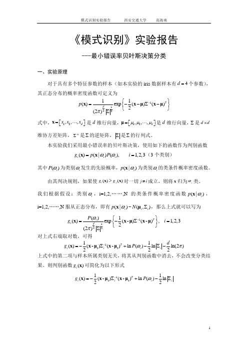
《模式识别》实验报告---最小错误率贝叶斯决策分类一、实验原理对于具有多个特征参数的样本(如本实验的iris 数据样本有4d =个参数),其正态分布的概率密度函数可定义为112211()exp ()()2(2)T d p π-⎧⎫=--∑-⎨⎬⎩⎭∑x x μx μ 式中,12,,,d x x x ⎡⎤⎣⎦=x 是d 维行向量,12,,,d μμμ⎡⎤⎣⎦=μ是d 维行向量,∑是d d ⨯维协方差矩阵,1-∑是∑的逆矩阵,∑是∑的行列式。
本实验我们采用最小错误率的贝叶斯决策,使用如下的函数作为判别函数()(|)(),1,2,3i i i g p P i ωω==x x (3个类别)其中()i P ω为类别i ω发生的先验概率,(|)i p ωx 为类别i ω的类条件概率密度函数。
由其判决规则,如果使()()i j g g >x x 对一切j i ≠成立,则将x 归为i ω类。
我们根据假设:类别i ω,i=1,2,……,N 的类条件概率密度函数(|)i p ωx ,i=1,2,……,N 服从正态分布,即有(|)i p ωx ~(,)i i N ∑μ,那么上式就可以写为1122()1()exp ()(),1,2,32(2)T i i dP g i ωπ-⎧⎫=-∑=⎨⎬⎩⎭∑x x -μx -μ对上式右端取对数,可得111()()()ln ()ln ln(2)222T i i i i dg P ωπ-=-∑+-∑-i i x x -μx -μ上式中的第二项与样本所属类别无关,将其从判别函数中消去,不会改变分类结果。
则判别函数()i g x 可简化为以下形式111()()()ln ()ln 22T i i i i g P ω-=-∑+-∑i i x x -μx -μ二、实验步骤(1)从Iris.txt 文件中读取估计参数用的样本,每一类样本抽出前40个,分别求其均值,公式如下11,2,3ii iii N ωωω∈==∑x μxclear% 原始数据导入iris = load('C:\MATLAB7\work\模式识别\iris.txt'); N=40;%每组取N=40个样本%求第一类样本均值 for i = 1:N for j = 1:4w1(i,j) = iris(i,j+1); end endsumx1 = sum(w1,1); for i=1:4meanx1(1,i)=sumx1(1,i)/N; end%求第二类样本均值 for i = 1:N for j = 1:4 w2(i,j) = iris(i+50,j+1);end endsumx2 = sum(w2,1); for i=1:4meanx2(1,i)=sumx2(1,i)/N; end%求第三类样本均值 for i = 1:N for j = 1:4w3(i,j) = iris(i+100,j+1); end endsumx3 = sum(w3,1); for i=1:4meanx3(1,i)=sumx3(1,i)/N; end(2)求每一类样本的协方差矩阵、逆矩阵1i -∑以及协方差矩阵的行列式i ∑, 协方差矩阵计算公式如下11()(),1,2,3,41i ii N i jklj j lk k l i x x j k N ωωσμμ==--=-∑其中lj x 代表i ω类的第l 个样本,第j 个特征值;ij ωμ代表i ω类的i N 个样品第j 个特征的平均值lk x 代表i ω类的第l 个样品,第k 个特征值;iw k μ代表i ω类的i N 个样品第k 个特征的平均值。
《模式识别》实验报告-贝叶斯分类
《模式识别》实验报告-贝叶斯分类一、实验目的通过使用贝叶斯分类算法,实现对数据集中的样本进行分类的准确率评估,熟悉并掌握贝叶斯分类算法的实现过程,以及对结果的解释。
二、实验原理1.先验概率先验概率指在不考虑其他变量的情况下,某个事件的概率分布。
在贝叶斯分类中,需要先知道每个类别的先验概率,例如:A类占总样本的40%,B类占总样本的60%。
2.条件概率后验概率指在已知先验概率和条件概率下,某个事件发生的概率分布。
在贝叶斯分类中,需要计算每个样本在各特征值下的后验概率,即属于某个类别的概率。
4.贝叶斯公式贝叶斯公式就是计算后验概率的公式,它是由条件概率和先验概率推导而来的。
5.贝叶斯分类器贝叶斯分类器是一种基于贝叶斯定理实现的分类器,可以用于在多个类别的情况下分类,是一种常用的分类方法。
具体实现过程为:首先,使用训练数据计算各个类别的先验概率和各特征值下的条件概率。
然后,将测试数据的各特征值代入条件概率公式中,计算出各个类别的后验概率。
最后,取后验概率最大的类别作为测试数据的分类结果。
三、实验步骤1.数据集准备本次实验使用的是Iris数据集,数据包含150个Iris鸢尾花的样本,分为三个类别:Setosa、Versicolour和Virginica,每个样本有四个特征值:花萼长度、花萼宽度、花瓣长度、花瓣宽度。
2.数据集划分将数据集按7:3的比例分为训练集和测试集,其中训练集共105个样本,测试集共45个样本。
计算三个类别的先验概率,即Setosa、Versicolour和Virginica类别在训练集中出现的频率。
对于每个特征值,根据训练集中每个类别所占的样本数量,计算每个类别在该特征值下出现的频率,作为条件概率。
5.测试数据分类将测试集中的每个样本的四个特征值代入条件概率公式中,计算出各个类别的后验概率,最后将后验概率最大的类别作为该测试样本的分类结果。
6.分类结果评估将测试集分类结果与实际类别进行比较,计算分类准确率和混淆矩阵。
模式识别方法二实验报告
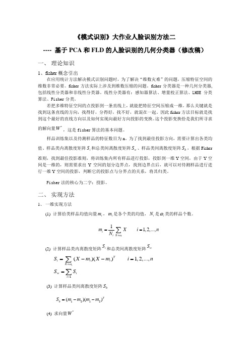
《模式识别》大作业人脸识别方法二---- 基于PCA 和FLD 的人脸识别的几何分类器(修改稿)一、 理论知识1、fisher 概念引出在应用统计方法解决模式识别问题时,为了解决“维数灾难”的问题,压缩特征空间的维数非常必要。
fisher 方法实际上涉及到维数压缩的问题。
fisher 分类器是一种几何分类器, 包括线性分类器和非线性分类器。
线性分类器有:感知器算法、增量校正算法、LMSE 分类算法、Fisher 分类。
若把多维特征空间的点投影到一条直线上,就能把特征空间压缩成一维。
那么关键就是找到这条直线的方向,找得好,分得好,找不好,就混在一起。
因此fisher 方法目标就是找到这个最好的直线方向以及如何实现向最好方向投影的变换。
这个投影变换恰是我们所寻求的解向量*W ,这是fisher 算法的基本问题。
样品训练集以及待测样品的特征数目为n 。
为了找到最佳投影方向,需要计算出各类均值、样品类内离散度矩阵i S 和总类间离散度矩阵w S 、样品类间离散度矩阵b S ,根据Fisher 准则,找到最佳投影准则,将训练集内所有样品进行投影,投影到一维Y 空间,由于Y 空间是一维的,则需要求出Y 空间的划分边界点,找到边界点后,就可以对待测样品进行进行一维Y 空间的投影,判断它的投影点与分界点的关系,将其归类。
Fisher 法的核心为二字:投影。
二、 实现方法1、 一维实现方法(1) 计算给类样品均值向量i m ,i m 是各个类的均值,i N 是i ω类的样品个数。
11,2,...,ii X im X i nN ω∈==∑(2) 计算样品类内离散度矩阵iS 和总类间离散度矩阵wS1()()1,2,...,i Ti i i X w ii S X m X m i nS Sω∈==--==∑∑(3) 计算样品类间离散度矩阵b S1212()()Tb S m m m m =--(4) 求向量*W我们希望投影后,在一维Y 空间各类样品尽可能地分开,也就是说我们希望两类样品均值之差(12m m -)越大越好,同时希望各类样品内部尽量密集,即希望类内离散度越小越好,因此,我们可以定义Fisher 准则函数:()Tb F Tw W S W J W W S W=使得()F J W 取得最大值的*W 为 *112()w WS m m -=-(5) 将训练集内所有样品进行投影*()Ty W X =(6) 计算在投影空间上的分割阈值0y在一维Y 空间,各类样品均值i m为 11,2,...,ii y imy i n N ω∈==∑样品类内离散度矩阵2i s和总类间离散度矩阵w s 22()ii iy sy mω∈=-∑21w ii ss==∑【注】【阈值0y 的选取可以由不同的方案: 较常见的一种是1122012N m N m y N N +=+另一种是121201ln(()/())22m m P P y N N ωω+=++- 】(7) 对于给定的X ,计算出它在*W 上的投影y (8) 根据决策规则分类0102y y X y y X ωω>⇒∈⎧⎨<⇒∈⎩2、程序中算法的应用Fisher 线性判别方法(FLD )是在Fisher 鉴别准则函数取极值的情况下,求得一个最佳判别方向,然后从高位特征向量投影到该最佳鉴别方向,构成一个一维的判别特征空间将Fisher 线性判别推广到C-1个判决函数下,即从N 维空间向C-1维空间作相应的投影。
模式识别基础实验报告资料

2015年12月实验一 Bayes 分类器的设计一、 实验目的:1. 对模式识别有一个初步的理解,能够根据自己的设计对贝叶斯决策理论算法有一个深刻地认识;2. 理解二类分类器的设计原理。
二、 实验条件:1. PC 微机一台和MATLAB 软件。
三、 实验原理:最小风险贝叶斯决策可按下列步骤进行:1. 在已知)(i P ω,)|(i X P ω,c i ,,1 =及给出待识别的X 的情况下,根据贝叶斯公式计算出后验概率:∑==c j jj i i i P X P P X P X P 1)()|()()|()|(ωωωωω c j ,,1 =2. 利用计算出的后验概率及决策表,按下式计算出采取i α决策的条件风险: ∑==c j j j i i X P X R 1)|(),()|(ωωαλα a i ,,1 =3. 对2中得到的a 个条件风险值)|(X R i α(a i ,,1 =)进行比较,找出使条件风险最小的决策k α,即:)|(min )|(,,1X R X R k c i k αα ==, 则k α就是最小风险贝叶斯决策。
四、 实验内容:假定某个局部区域细胞识别中正常(1ω)和非正常(2ω)两类先验概率分别为: 正常状态:)(1ωP =0.9;异常状态:)(2ωP =0.1。
现有一系列待观察的细胞,其观察值为x :-3.9847 -3.5549 -1.2401 -0.9780 -0.7932 -2.8531-2.7605 -3.7287 -3.5414 -2.2692 -3.4549 -3.0752-3.9934 2.8792 -0.9780 0.7932 1.1882 3.0682-1.5799 -1.4885 -0.7431 -0.4221 -1.1186 4.2532)|(1ωx P )|(2ωx P 类条件概率分布正态分布分别为(-2,0.25)(2,4)。
决策表为011=λ(11λ表示),(j i ωαλ的简写),12λ=6, 21λ=1,22λ=0。
模式识别实验【范本模板】

《模式识别》实验报告班级:电子信息科学与技术13级02 班姓名:学号:指导老师:成绩:通信与信息工程学院二〇一六年实验一 最大最小距离算法一、实验内容1. 熟悉最大最小距离算法,并能够用程序写出。
2. 利用最大最小距离算法寻找到聚类中心,并将模式样本划分到各聚类中心对应的类别中.二、实验原理N 个待分类的模式样本{}N X X X , 21,,分别分类到聚类中心{}N Z Z Z , 21,对应的类别之中.最大最小距离算法描述:(1)任选一个模式样本作为第一聚类中心1Z 。
(2)选择离1Z 距离最远的模式样本作为第二聚类中心2Z 。
(3)逐个计算每个模式样本与已确定的所有聚类中心之间的距离,并选出其中的最小距离.(4)在所有最小距离中选出一个最大的距离,如果该最大值达到了21Z Z -的一定分数比值以上,则将产生最大距离的那个模式样本定义为新增的聚类中心,并返回上一步.否则,聚类中心的计算步骤结束。
这里的21Z Z -的一定分数比值就是阈值T ,即有:1021<<-=θθZ Z T(5)重复步骤(3)和步骤(4),直到没有新的聚类中心出现为止。
在这个过程中,当有k 个聚类中心{}N Z Z Z , 21,时,分别计算每个模式样本与所有聚类中心距离中的最小距离值,寻找到N 个最小距离中的最大距离并进行判别,结果大于阈值T 是,1+k Z 存在,并取为产生最大值的相应模式向量;否则,停止寻找聚类中心。
(6)寻找聚类中心的运算结束后,将模式样本{}N i X i ,2,1, =按最近距离划分到相应的聚类中心所代表的类别之中。
三、实验结果及分析该实验的问题是书上课后习题2。
1,以下利用的matlab 中的元胞存储10个二维模式样本X {1}=[0;0];X{2}=[1;1];X {3}=[2;2];X{4}=[3;7];X{5}=[3;6]; X{6}=[4;6];X{7}=[5;7];X{8}=[6;3];X{9}=[7;3];X{10}=[7;4];利用最大最小距离算法,matlab 运行可以求得从matlab 运行结果可以看出,聚类中心为971,,X X X ,以1X 为聚类中心的点有321,,X X X ,以7X 为聚类中心的点有7654,,,X X X X ,以9X 为聚类中心的有1098,,X X X 。
模式识别课程实验报告

模式识别课程实验报告学院专业班级姓名学号指导教师提交日期1 Data PreprocessingThe provide dataset includes a training set with 3605 positive samples and 10055 negative samples, and a test set with 2043 positive samples and 4832 negative samples. A 2330-dimensional Haar-like feature was extracted for each sample. For high dimensional data, we keep the computation manageable by sampling , feature selection, and dimension reduction.1.1 SamplingIn order to make the samples evenly distributed, we calculate the ratio of negative samples and positive samples int test set. And then randomly select the same ratio of negative samples in training set. After that We use different ratios of negative and positive samples to train the classifier for better training speed.1.2 Feature SelectionUnivariate feature selection can test each feature, measure the relationship between the feature and the response variable so as to remove unimportant feature variables. In the experiment, we use the method sklearn.feature_selection.SelectKBest to implement feature selection. We use chi2 which is chi-squared stats of non-negative features for classification tasks to rank features, and finally we choose 100 features ranked in the top 100.2 Logistic regressionIn the experiment, we choose the logistic regression model, which is widely used in real-world scenarios. The main consideration in our work is based on the binary classification logic regression model.2.1 IntroductionA logistic regression is a discriminant-based approach that assumes that instances of a class are linearly separable. It can obtain the final prediction model by directly estimating the parameters of the discriminant. The logistic regression model does not model class conditional density, but rather models the class condition ratio.2.2 processThe next step is how to obtain the best evaluation parameters, making the training of the LR model can get the best classification effect. This process can also be seen as a search process, that is, in an LR model of the solution space, how to find a design with our LR model most match the solution. In order to achieve the best available LR model, we need to design a search strategy.The intuitive idea is to evaluate the predictive model by judging the degree of matching between the results of the model and the true value. In the field of machine learning, the use of loss function or cost function to calculate the forecast. For the classification, logistic regression uses the Sigmoid curve to greatly reduce the weight of the points that are far from the classification plane through the nonlinear mapping, which relatively increases the weight of the data points which is most relevant to the classification.2.3 Sigmoid functionWe should find a function which can separate two in the two classes binary classification problem. The ideal function is called step function. In this we use the sigmoid function.()z e z -+=11σWhen we increase the value of x, the sigmoid will approach 1, and when we decrease the value of x, the sigmoid will gradually approaches 0. The sigmoid looks like a step function On a large enough scale.2.4 gradient descenti n i i T i x x y L ∑=+--=∂∂-=1t t1t ))(()(θσαθθθαθθThe parameter α called learning rate, in simple terms is how far each step. this parameter is very critical. parameter σis sigmoid function that we introduce in 2.3.3 Train classifierWe use the gradient descent algorithm to train the classifier. Gradient descent is a method of finding the local optimal solution of a function using the first order gradient information. In optimized gradient rise algorithm, each step along the gradient negative direction. The implementation code is as follows:# calculate the sigmoid functiondef sigmoid(inX):return 1.0 / (1 + exp(-inX))#train a logistic regressiondef trainLogisticRegression(train_x, train_y, opts):numSamples, numFeatures = shape(train_x)alpha = opts['alpha'];maxIter = opts['maxIter']weights = ones((numFeatures, 1))# optimize through gradient descent algorilthmfor k in range(maxIter):if opts['optimizeType'] == 'gradDescent': # gradient descent algorilthm output = sigmoid(train_x * weights)error = train_y - outputweights = weights + alpha * train_x.transpose() * error return weightsIn the above program, we repeat the following steps until the convergence:(1) Calculate the gradient of the entire data set(2) Use alpha x gradient to update the regression coefficientsWhere alpha is the step size, maxIter is the number of iterations.4 evaluate classifier4.1 optimizationTo find out when the classifier performs best, I do many experiments. The three main experiments are listed below.First.I use two matrix types of data to train a logistic regression model using some optional optimize algorithm, then use some optimization operation include alpha and maximum number of iterations. These operations are mainly implemented by this function trainLogisticRegression that requires three parameters train_x, train_y, opts, of which two parameters are the matrix type of training data set, the last parameter is some optimization operations, including the number of steps and the number of iterations. And the correct rate as follows:When we fixed the alpha, change the number of iterations, we can get the results as shown below:Red: alpha = 0.001Yellow: alpha = 0.003Blue: alpha = 0.006Black: alpha = 0.01Green: alpha = 0.03Magenta: alpha = 0.3This line chart shows that if the iterations too small, the classifier will perform bad. As the number of iterations increases, the accuracy will increase. And we can konw iterations of 800 seems to be better. The value of alpha influences the result slightly. If the iterations is larger then 800, the accuracy of the classifier will stabilize and the effect of the step on it can be ignored.Second.When we fixed the iterations, change the alpha, we can get the results as shown below:This line chart shows when the number of iterations is larger 800, the accuracy is relatively stable, with the increase of the alpha, the smaller the change. And when the number of iterations is small, for example, the number of times is 100, the accuracy is rather strange, the accuracy will increase with the increase of alpha. We can know that when the number of iterations is small, even if the alpha is very small, its accuracy is not high. The number of iterations and the alpha is important for the accuracy of the logical regression model training.Third.The result of the above experiment is to load all the data to train the classifier, but there are 3605 pos training data but 10055 neg training data. So I am curious about whether can I use less neg training data to train the classifier for better training speed.I use the test_differentNeg.py to does this experiment:Red: iterations = 100 Yellow: iterations = 300 Blue: iterations = 800 Black: iterations = 1000The line chart shows that the smaller the negative sample, the lower the accuracy. However, as the number of negative samples increases, the accuracy of the classifier.I found that when the number of negative samples is larger 6000, the accuracy was reduced and then began to increase.4.2 cross-validationWe divided the data set into 10 copies on average,9 copies as a training set and 1 copies as a test set.we can get the results as shown below:Red: alpha = 0.001Yellow: alpha = 0.003Blue: alpha = 0.006Black: alpha = 0.01Green: alpha = 0.03Magenta: alpha = 0.3This figure shows that if the iterations too small, the classifier will perform bad. Asthe number of iterations increases, the accuracy will increase. And we can konw iterations of 1000 seems to be better. The value of alpha influences the result slightly.If the iterations is larger then 1000, the accuracy of the classifier will achieve 84% and stable. And the effect of the step on it can be ignored.5 ConclusionIn this experiment, We notice that no matter before or after algorithm optimization,the test accuracy does not achieve our expectation. At first the accuracy of LR can reach 80%. After optimization, the accuracy of LR can reach 88%. I think there are several possible reasons below:(1) The training set is too small for only about 700 samples for active training sets, while the negative training set has only 800 samples;(2) We did not use a more appropriate method to filter the samples;(3) The method of selecting features is not good enough because it is too simple;(4) Dimension reduction does not be implemented, so that The high dimension of features increases the computation complexity and affects the accuracy;(5) The test sets may come from different kinds of video or images which are taken from different areas.(6) The number of iterations is set too small or the alpha is set too small or too large. These questions above will be improved in future work.In this project, we use Logistic regression to solve the binary classification problem. Before the experiment, we studied and prepared the algorithm of the LR model and reviewed other machine learning models studied in the pattern recognition course. In this process, we use python with a powerful machine learning library to implement, continue to solve the various problems, and optimize the algorithm to make the classifier perform better. At the same time, we also collaborate and learn from each other. Although the project takes us a lot of time, We have consolidated the theoretical knowledge and have fun in practice.。
模式识别学习报告(团队)
模式识别学习报告(团队)
简介
本报告是我们团队就模式识别研究所做的总结和讨论。
模式识别是一门关于如何从已知数据中提取信息并作出决策的学科。
在研究过程中,我们通过研究各种算法和技术,了解到模式识别在人工智能、机器研究等领域中的重要性并进行实践操作。
研究过程
在研究过程中,我们首先了解了模式识别的基本概念和算法,如KNN算法、朴素贝叶斯算法、决策树等。
然后我们深入研究了SVM算法和神经网络算法,掌握了它们的实现和应用场景。
在实践中,我们使用了Python编程语言和机器研究相关的第三方库,比如Scikit-learn等。
研究收获
通过研究,我们深刻认识到模式识别在人工智能、机器研究领域中的重要性,了解到各种算法和技术的应用场景和优缺点。
同时我们也发现,在实践中,数据的质量决定了模型的好坏,因此我们需要花费更多的时间来处理数据方面的问题。
团队讨论
在研究中,我们也进行了很多的团队讨论和交流。
一方面,我们优化了研究方式和效率,让研究更加有效率;另一方面我们还就机器研究的基本概念和算法的前沿发展进行了讨论,并提出了一些有趣的问题和方向。
总结
通过学习和团队讨论,我们深刻认识到了模式识别在人工智能和机器学习领域中的核心地位,并获得了实践经验和丰富的团队协作经验。
我们相信这些学习收获和经验会在今后的学习和工作中得到很好的应用。
- 1、下载文档前请自行甄别文档内容的完整性,平台不提供额外的编辑、内容补充、找答案等附加服务。
- 2、"仅部分预览"的文档,不可在线预览部分如存在完整性等问题,可反馈申请退款(可完整预览的文档不适用该条件!)。
- 3、如文档侵犯您的权益,请联系客服反馈,我们会尽快为您处理(人工客服工作时间:9:00-18:30)。
机器学习实验报告模板
题目:XXX实验报告
班级:XXX班
专业:XXXXXX
姓名:XXX
学号:XXXXXXXX
、实验目的
1、 验证抽样左理:设时间连续信号f (t),其最髙截止频率为fin ,如果用时间间隔 为T<=l/2fiii 的开
关信号对f (t)进行抽样时,则f (t)就可被样值信号唯一地表 /Jso
2、 降低或提髙抽样频率,观察对系统的影响
二、实验原理
抽样定理:
一个频带限制在((),九)赫内的时间连续信号〃", 如果以701/(2儿)秒的间隔对它进行等间隔(均匀) 抽样,则〃砒)将被所得到的抽样值完全确定。
/K 爪爪爪: -2 —
",
-5
3. 3.
2"・
S>2 %
尸2
/MVyyrv
3,・? 3、 A/YYV\ ■
图一抽样定理示意图
从图中可以看岀,当£>=2血时,不会发生频域混叠现象,使用一个匹配的低通滤 波
匹
2 低通滤也件
波器
无失真抽样的
要求
“5(%)
由样值序列町无 火貝的恢圮出脈 來的模拟信号
抽样左理示意图
:
器即可无失真的恢复出原信号,当£<2翕时,会发生频域混叠现象,这时,恢复的信号失真。
三、模型结构
实验所需模块连接图如下所示:
1S,1000Hz.分别为lOhz, 121iz, 14hz,再利用脉冲发生器产生抽样脉冲,将脉宽设巻为lessee, 脉冲频率分别设置为20hz, 30hz, 50hzo
对三个信号做加法,所得信号的最高频率为14hz,由抽样徒理得抽样脉冲的频率应大 于等于
28hz
可使得恢复信号无失真,所以选择与
28hz
相近的30hz.并取抽样脉冲频率为 20hz 和
50hz
做
比较,验证抽样定理。
令相加所得信号与抽样脉冲相乘,得到的结果即为时间离散的抽样序列。
最后将抽样序 列通过五阶巴特沃斯低通滤波器,由于信号最髙频率为14hz,所以取滤波器的截止频率为 14hz.将恢复信号与原信号作比较,比较不同抽样频率带来的影响。
四、实验步骤
(1)
按照实验所需模块连接图,连接各个模块
(2)
进行系统左时设置:起始时间设为0,终止时间设为Is.抽样率设为lkliz.
图二模块连接图
元件编号
属性
类型
参数设置
0,1,2
Source Sin usiod
Amp=lV ; Rate=10/12/14Hz
3 Adder
4 Multipler
7 Operator Lin ear Sys
Butterworth z 5 Poles /fc=14Hz 5,6,8
Sink
9
Operator
Pluse Train
Amp=lVt f=30hz» Width=0.01sec
傅︕r
频
信︔
菠lvhz ?t
为
别30
ec
设
hl
A
区
• ................ • ... SystemView by ELANIX .
图三系统定时设置示意图
(3)设置各个模块的参数:
①信号源部分:使用三个正弦波信号源产生三个正弦波,其频率分别为10hz,
12hz, 14hzo
② 抽样脉冲发生器:利用脉冲发生器产生抽样脉冲,将脉宽设置为lessee, 脉冲频率分别设置为20hz. 3Ohz, 50112,
图五抽样脉冲发生器设置示意图
③低通滤波器:五阶巴特沃斯低通滤波器,截止频率14112
图六低通滤波器设置示意图
(4)观察输出波形,更改抽样脉冲发生器的频率,比较试验结果。
五、实验结果
(1)当抽样频率为30hz时,实验结果如下图,最上方的图为原基带信号,中间图为经过低通滤波器后的输岀波形,最下方图为脉冲序列和信号源信号相乘后的波形。
图七采样频率为20hz波形图
由上图可知,采样后恢复的信号与基带信号几乎一模一样,只是有一左的时延,根据以上实验结果,我们可知,当fs=2fin (本处为略大于)时,可以由抽样序列唯一的恢复原信号。
(原信号的最高频率fiii=14hz)
(2)当抽样频率为50hz时,实验结果如下图,最上方的图为原基带信号,中间图为
经过低通滤波器后的输出波形,最下方图为脉冲序列和信号源信号相乘后的波
由上图可知,采样后恢复的信号与基带信号几乎一模一样,只是有一左的时延.根据以上实验结果,我们可知,当fs>2fm时,可以由抽样序列唯一的恢复原信号。
(原信号的最髙频率fhi=14hz)(3)当抽样频率为20hz时,实验结果如下图,最上方的图为原基带信号,中间图为经过低通滤波器后的输出波形,最下方图为脉冲序列和信号源信号相乘后的波形。
图九采样频率为20hz波形图
由上图可知,釆样后恢复的信号岀现明显的失真,根据以上实验结果,我们可知,当fs<2fiii时,输出信号发生较大的失真,已经无法恢复原信号。
(原信号的最高频率=14hz)(4):当抽样频率为30hz,将抽样脉冲的脉宽加大(15e-3sec),实验结果如下图,最上方的图为原基带信号,中间图为经过低通滤波器后的输出波形,最下方图为脉冲序列和
信号源信号相乘后的波形。
根据以上实验结果,我们可知,抽样序列的脉宽过大时,会导致采样信号的时间离散型不好,但是根据新的这样的采样信号,还是可以恢复出原信号的。
(原信号的最高频率=14hz)
图十抽样脉冲的脉宽加大后波形图
(5)当抽样频率为30hz,低通滤波器的阶数降低(降低到2阶),实验结果如下图, 最上方的图为原基带信号,中间图为经过低通滤波器后的输岀波形,最下方图为脉冲序列和信号源信号相乘后的波形。
六、实验讨论与分析
从实验结果可以看岀,抽样频率为30hz,原信号的频率为1411Z,满足抽样立理。
抽样后的信号通过低通滤波器后,恢复出的信号波形与原基带信号相同,可以无失貞•的恢复原信号;当抽样频率为50hz时,依然满足抽样泄理,此时也可以无失真的恢复原信号;当抽样频率为20hz时,不满足抽样泄理,此时由于频域混叠现象,输出信号发生了较大的失真,不可以无失真的恢复原信号。
由此可知,如果抽样的时间间隔T<=l/2fin,则所得样值序列含有原基带信号的全部信息,从该样值序列可以无失真地恢复成原来的基带信号。
验证了抽样泄理。
另外,要选择过渡带宽较小的滤波器,减小信号带外因素的影响。
通过本次实验,我加深了对于抽样泄理的理解,进一步了解了采样泄理的原理和意义作用,也初步掌握了SystemView的使用,了解了软件的基本用法。
更重要的是,通过此次的实验对于通信原理的课程学习带来很大的帮助,将理论与实践结合,更加深了理论学习的印象。
对于课本上的知识也有了更深的理解和新的认识。
1
> °
s
I *
----- 产
■ -—
—
)3
■OH
MV
1 1
/)\
二/、■才/
1
— -- K
——
(
K,
^==
■ ■■ ■
=====
rn~
n>t0>)
I \■
* \ - 、/
J严
WH
■5M
/
、~z\—r■/ \
\ //J'/、/
w
■
WH
a
BkJ—ft
q A-v-
_____
T-J
r
=
—
厂
■
98t=^=l
根据以上实验结果,我们可知,由于采样频率接近于2fin,所以当滤波器的带外特性不好,衰减过慢的时候,高频的信号不能保证完全滤除。
这时候恢复的信号也是失真的。
(原信号的最高频率=141iz)
七、实验意见与建议
1、希望可以加入在频域观察信号波形的实验,很多在时域不是很好发现的情况,在频域
可以一目了然的发现到。
2、我发现实验三的电路连接可能不够合理,PN序列发生器产生的是双极性NRZ 信号,而
我们需要的是双极性冲激序列。
具体的改进方案请见实验三实验结论部分。
3、希望课程时间安排的长一些,能让老师有更多的时间进行讲解和指导,同时也能让我
们有更多的时间去完成实验。