trace32使用手册
TRACE32 iAMP 双核调试应用说明书
Application Note for iAMP Debugging Release 09.2023TRACE32 Online HelpTRACE32 DirectoryTRACE32 IndexTRACE32 Documents ...................................................................................................................... Multicore Debugging ..................................................................................................................... Application Note for iAMP Debugging . (1)SMP, iAMP or AMP? (3)iAMP Setup (7)Example iAMP Setup10Version 09-Oct-2023 11-Nov-2021New manual.SMP, iAMP or AMP?TRACE32 offers various configuration possibilities for debugging multi-core target systems. This chapter explains the basic differences between:•SMP (Symmetrical MultiProcessig)•iAMP (integrated Asymmetrical MultiProcessing)•AMP (Asymmetrical MultiProcessig)This application note focuses on iAMP. It gives you a basic overview of the iAMP concept and helps you to choose the right configuration for your setup. For further details about iAMP and the commands used here, you can also see the “General Reference Guide” (general_ref_<x>.pdf) or contact**********************.If you want to create a new TRACE32 setup for any multicore system, one of the very first decisions you have to make is “AMP or SMP or iAMP?”. In some cases, only one of the possibilities is supported by TRACE32, for example: if you have several cores of different architectures (like one Arm core, one Xtensa core and one RISC-V core), then AMP is the only possible option. But in many cases, you have a choice.Let’s first take a look at the key properties of the three concepts:•All cores have the same instruction set.•All cores use the same instance of an OS (when not bare-metal and unless you are using a hypervisor (“Hypervisor Debugging User Guide” (hypervisor_user.pdf)).•All cores use the same memory model and same address translations (unless you are using a hypervisor).•All cores share the same physical and logical address space.•All cores share the same debug symbols (typically the same elf file).•All cores are debugged from a single TRACE32 PowerView instance. Y ou can have up to 1024cores.•TRACE32 starts and stops all cores simultaneously (even though you can temporarily single out one core for independent start/stop).iAMP (integrated asymmetrical multiprocessing):•All cores have the same instruction set.•There are typically multiple OS instances (if not bare metal).•There is just one global physical address space but each OS maintains its own set of virtual address spaces.•All cores are debugged from a single TRACE32 PowerView GUI. The number of cores is limited just by the core architecture used and can be very high.•TRACE32 allows to group cores logically into machines; this grouping depends on the logical structure of the system under debug - each machine consists of one or more cores. Up to30machines are possible.•Each machine has its own OS instance (if not bare metal).•Each machine has its own memory model, address translations and debug symbols.•TRACE32 starts and stops all cores simultaneously (even though you can temporarily single out one core for independent start/stop).•AMP can bundle single cores, as well as SMP and iAMP subsystems.•Mixing of different core architectures with different instruction sets is possible.•Each core/subsystem has its own TRACE32 PowerView GUI.•Each core/subsystem has its own (different) memory models, address translations, elf files and debug symbols.•Each core/subsystem can have its own physical address space.•Each core/subsystem has its own logical address spaces.•Each core/subsystem starts and stops independently but can also be synchronized.•AMP is limited to 16 TRACE32 PowerView GUIs.An example of an AMP system that bundles single cores, an SMP and an iAMP subsystem can be found on page10.The most important questions for the decision are:•Do all my cores use the same instruction set?If not, it is definitely AMP.•Do all my cores of the same instruction set run a single instance of OS?If yes, these cores form an SMP (sub)system.•Are there SMP subsystems and single cores of the same instruction set? Does it make sense to configure them as an iAMP system and debug them from a single TRACE32PowerView instance?Y es, if they are all using a global physical address space.Y es, if they logically belong together; that means they work together or in parallel on the same tasks.Y es, if you want or need to reduce the number of TRACE32 PowerView instances.The following table provides a systematic overview:SMP AMP iAMP Homogeneous cores (cores of the same instruction set)✓✓✓Heterogeneous cores✓Single TRACE32 instance/GUI✓✓Multiple TRACE32 instances/GUIs 16Hypervisor with statically assigned guests (core identity)✓✓✓Hypervisor with dynamic core assignment (core sharing)✓SMP OS (a single OS managing multiple cores)✓Multiple OSes without hypervisor✓Synchronous run✓✓✓Asynchronous run✓iAMP is available for selected core architectures like Arm, Hexagon and T riCore. If you need iAMP and your platform does not support it yet, please contact your local Lauterbach representative or**********************.Some of the decision criteria are easy to evaluate (like more than 16 CPUs) but some of them are quite fuzzy - talking to Lauterbach representative or Lauterbach support might help you with the decision.iAMP SetupThe basis for an iAMP system is that cores are grouped into machines.The SYStem.Option.MACHINESPACES ON command creates the basis for this.All cores that use the same instance of an OS (when not bare-metal) can be grouped and assigned to a machine by the TASK.Create.MACHINE command.Example :This will create two machines, each of them with two cores. Their setup can be then displayed using the commandTASK.List.MACHINES :The columns name and cores in the screenshot are self-explaining, ‘mid’ displays the machine ID, other columns are not relevant for our example.It may be necessary to use the CORE.ASSIGN command beforehand to assign the physical cores to the logical cores of the iAMP system.Use the command CORE.select <logical_core> to switch to the core of interest and the TRACE32PowerView GUI will display the system information from the perspective of the selected core. T o understand how this works, think that “the machine is never selected directly but always follows selected core”.By default, all cores are started and stopped simultaneously , but you can single out a single core for independent start/stop by using the CORE.SINGLE <logical_core> command.The CORE.select command without an argument can be used to reverse this selection after the core is stopped.It is imperative to ensure that the symbols loaded by any of the Data.LOAD.* commands will be added to the right machine space. When loading executables and symbol information, the safest way is to explicitly select the core to which the executable belongs – it then explicitly defines both the core and machine. One of the reasons is that registers like PC might be pre-initialized during Data.LOAD so by selecting the correct core it becomes clear where the register(s) are to be set:TASK.Create.MACHINE , 0. "main0" /CORE 0. 1.TASK.Create.MACHINE , 1. "main1" /CORE 2. 3.CORE.select 0.Data.LOAD.Elf application_subsystem0.elf CORE.select 2.Data.LOAD.Elf application_subsystem1.elf /NoClearOn the other hand, when you load only symbol information and no register content, it is sufficient to specify only the machine; knowledge of the specific core is not required. T o specify only the machine, use theloading offset parameter to Data.LOAD.* where this offset contains the machine number. In most cases you use zero as offset (unless you need to shift the data to another base address).Loading symbols using the machine ID makes them machine aware as can be seen in the image below.The machine name can be explicitly specified in a symbol name using triple-backslash (“\\\”) syntax.Example :This command will show the source of the symbol start from the module Global on the machine named main1.The general format for symbol names becomes:[\\\<machine_name>]\\[<program_name>]\[<module_name>]\<symbol_name>Both <program_name> and <module_name> may be omitted if there is no ambiguity with another symbol but the appropriate backslashes must remain to indicate where they were, for example:\\\<machine_name>\\\<symbol_name>So, our example of \\\main1\\Global\start now becomes \\\main1\\\\startWhen you activate the iAMP mode, the behavior of many commands changes. The commands now also consider the correct machine scope, for example:Data.LOAD.Elf application_subsystem0.elf 0x0:::0 /NoCODE /NoRegData.LOAD.Elf application_subsystem1.elf 0x1:::0 /NoClear /NoCODE /NoRegNOTE:This concept is extended to allow you to access a logical address on any machine and works like this:[<access_class>:][<machine_id>:::]<address_offset> Example:P:1:::0x1234000 means program address P:0x1234000 on machine 1.R:0:::0x81021864 means AArch32 Arm code at address R:0x81021864 on machine 0.List.Asm \\\main1\\\Global\startNormally, MMU.DUMP.TLB shows the only TLB in the system (where available). With iAMP, the contents displayed by MMU.DUMP.TLB will update after every change of machine and always show the TLB of the currently selected machine.The program counter is now shown everywhere with the machine number included - like in this CORE.List window:The machine number is also included in many other outputs and windows, almost everywhere where you see an address. The screenshot below shows the sYmbol.List.SECtion window. It can be seen that sections from all machines and all addresses include the machine number.Example iAMP SetupAssume the following system, based on a TDA4VM chip from T exas Instruments:•Four Cortex-R5 cores, grouped in two core pairs, called “main0” and “main1”. These four cores form our example iAMP system.Each core pair has its own symbols and ELF file (app_ddr.elf and app_sram.elf ).Both core pairs use logical memory but have their own translations.•In addition to that, there is also a Cortex-M3 core (“master”), Cortex-R5 (“mcu”) based SMP subsystem and a TI C71x (“dsp”) on the chip, which all need to be debugged as well.Four TRACE32 PowerView GUIs are needed to debug this AMP system:1.GUI to control the Cortex-R5 based iAMP subsystem 2.GUI to control a single Cortex-M33.GUI to control the Cortex-R5 based SMP subsystem4.GUI to control a single C71x DSPTRACE32 PowerDebugDebug Port®iAMP main0 + main1Cortex-M3masterSMP 2x Cortex-R5mcuC71x dspApplication Note for iAMP Debugging | 11©1989-2023 L auterbach So, let's focus on the iAMP subsystem - we want to preload all elf files, execute all startups immediately after loading, and then start the execution of all cores/machines from the symbol main simultaneously. For this setup, the following script can be used:The other subsystems of SoC are initialized as usual with their own scripts.The structure of the whole system can be then displayed via the command TargetSystem ALL .sYmbol.RESetSYStem.Option.MACHINESPACES ONTASK.CREATE.MACHINE , 0. "main0" /CORE 0. 1.TASK.CREATE.MACHINE , 1. "main1" /CORE 2. 3.CORE.select 0.Data.LOAD.Elf app_ddr.elfCORE.select 2.Data.LOAD.Elf app_ram.elf /NoClearCORE.SINGLE 0. ; enter single core execution mode Go mainWAIT !STATE.RUN()CORE.SINGLE 2. ; enter single core execution mode Go mainWAIT !STATE.RUN()CORE.select 0. ; leaving single core execution mode PRINT "Now we are ready to debug from main"。
trace32使用手册
置调试源文件路径。
四、 观察/修改寄存器 从主菜单区点击“CPU->CPU Registers” ,打开内核寄存器窗口,如下图所示。 Pic11. 内核寄存器观察菜单
Pic12. 内核寄存器窗口
从 Pic12 所示的内核寄存器窗口, 用户能够观察处理器内核寄存器的值。 如果用户想 修改某一个寄存器的值, 只要双击寄存器名右边的值, 在行命令输入区就会出现相应 寄存器值修改的命令,紧接着输入十六进制的值(如,0x12345678)并回车就可以了。 下图是以修改寄存器 R2 的值为例,在行命令输入区出现的命令。 Pic13. 修改内核寄存器
Pic29 中红框内的单选钮 IMASKASM 和 IMASKHLL 选择之后,单步时就会屏蔽中断。 用户也可以通过命令 sys.o imaskasm on 和 sys.o imaskhll on 来设置这两个选项。
十、 设置软件断点 设置软件断点可以在命令行输入命令 break.set <address> /soft 来实现,在命令中的 <address>代表程序地址,可以是程序中的函数名等符号。如下图所示。 Pic30. 用命令设置软件断点
六、 下载程序 使用 data.load 命令实现程序下载的功能,如下图所示。 Pic20. 下载程序 上图中,“elf”指示所下载的程序的文件格式,“/v”指示程序下载完成之后进行校验。
Trace32-ICD使用说明

Trace32-ICD使用说明作者:***日期:2008-8-11版本:V-1.0一、编写目的通过对该文档的阅读,能够掌握Trace32-ICD的软、硬件安装,使用Trace32-ICD进行flash擦除,程序下载,并熟悉在线调试。
二、T RACE32硬件的连接Trace32的硬件连接如下图所示:图2.1注意事项:电源打开/关闭时的正确顺序:打开:先调试器,再目标机。
关闭:先目标机,再调试器。
三、TRACE32软件的安装3.1 TRACE32-ICD软件包安装1、首先获取安装软件包,包括:Trace32安装包和USB Driver。
2、安装Trace软件包,运行..\ trace32\setup.bat批处理文件或..\trace32\bin\setup\setup.exe文件,系统自动安装,在安装过程中进行如下选择。
图 3.1 图3.2图3.3其他选项基本默认。
3.2 USB驱动安装正确连接Trace后,系统会自动提示发现硬件需要进行驱动。
此时选择驱动程序所在目录。
路径为..\ trace32\bin。
如图3.4所示。
图3.4四、Flash的擦除与下载程序由于手机在下载版本过程中死机或掉电造成手机无法正常启动,并且使用我们单位的ZXPST与QPST都无法进行版本下载,并且QXDM和ZXPST通过COM1接口也无法找到手机,于是无法下载。
在这种情况下我们可以使用Trace32-ICD进行Flash的擦除和程序下载。
4.1 设置环境CPU环境设置在SYStem窗口,SYStem窗口提供所有CPU特定的设置。
使用CPU菜单中的System Settings…打开SYStem窗口如图4.1所示。
需要配置主要包括CPU、时钟和UP加电,CPU选择ARM926EJ,时钟JtagClock选择Ttck,然后进行加电UP,如果连接一切都正常,设置这几项就可以了。
如图4.1所示:图4.1注意事项:如果UP不上出现如下错误emulation debug port fail,说明硬件连接不正确。
Trace32 PXROS用户手册和版本帮助(MANUAL)说明书
OS Awareness Manual PXROS Release 09.2023TRACE32 Online HelpTRACE32 DirectoryTRACE32 IndexTRACE32 Documents ......................................................................................................................OS Awareness Manuals ................................................................................................................OS Awareness Manual PXROS (1)History (3)Overview (3)Brief Overview of Documents for New Users4 Supported Versions4Configuration (5)Quick Configuration Guide5 Hooks & Internals in PXROS6Debug Features (7)Display of Kernel Resources7 Task Stack Coverage7 Task-Related Breakpoints8 Task Context Display9 SMP Support9 Dynamic Task Performance Measurement10 PXROS Specific Menu11Trace Features (12)Task Runtime Statistics12 Function Runtime Statistics13 CPU Load Analysis15 PXROS Specific Menu for Tracing16PXROS Commands (17)TASK.ListmbX Display mailboxes17 TASK.ListObject List objects17 TASK.ListObj.DeLaY Display delay objects18 TASK.ListObj.MailBoX Display mailboxes18 TASK.ListObj.MemClass Display memory classes19 TASK.ListObj.MeSsaGe Display message objects19 TASK.ListObj.OPool Display object pools20 TASK.ListTask Display task table20Version 09-Oct-2023 History08-Oct-19Added support for PXROS v7.OverviewThe OS Awareness for PXROS contains special extensions to the TRACE32 Debugger. This manual describes the additional features, such as additional commands and statistic evaluations.Brief Overview of Documents for New UsersArchitecture-independent information:•“Training Basic Debugging” (training_debugger.pdf): Get familiar with the basic features of a TRACE32 debugger.•“T32Start” (app_t32start.pdf): T32Start assists you in starting TRACE32 PowerView instances for different configurations of the debugger. T32Start is only available for Windows.•“General Commands” (general_ref_<x>.pdf): Alphabetic list of debug commands.Architecture-specific information:•“Processor Architecture Manuals”: These manuals describe commands that are specific for the processor architecture supported by your Debug Cable. T o access the manual for your processorarchitecture, proceed as follows:-Choose Help menu > Processor Architecture Manual.•“OS Awareness Manuals” (rtos_<os>.pdf): TRACE32 PowerView can be extended for operating system-aware debugging. The appropriate OS Awareness manual informs you how to enable theOS-aware debugging.Supported VersionsCurrently PXROS is supported for the following versions:•PXROS 4.x on C166/C167, PowerPC and T riCore•PXROS 5.x, 6.x, 7.x and 8.x on TriCoreConfigurationThe TASK.CONFIG command loads an extension definition file called “pxros.t32” (directory“~~/demo/<arch>/kernel/pxros”). It contains all necessary extensions.TASK.CONFIG ~~/demo/<arch>/kernel/pxros/pxros.t32 [<magic_address>[<args>]]<magic_address>Specifies a memory location that contains the current running task. Thisaddress can be found at “...”.<args>The configuration requires additional arguments, that are:•<sleep>: Currently not used, specify “0”•<dpp>: (only on C166) The first argument configures the datapage settings of the application. Specify a long word which leastsignificant byte is the dpp0 content and which most significant byteis the dpp3 content. E.g. '03060500' means dpp0=0, dpp1=5,dpp2=6 and dpp3=3. If you don't know the dpp settings of yourapplication, just start it for a while and check in the 'register' com-mand the dpp's. Note that the dpp settings must be adapted to everysingle application.•<internal>: The next three arguments are PXROS internal struc-tures. Specify “__PxTasklist __PxTaskRdyFromRdy__PxUsedObjs”.Without any parameters, the debugger tries to locate the internals of PXROS automatically. For this purpose, the kernel symbols must be loaded and accessible at any time the OS Awareness is used (see also “Hooks & Internals”).If you want to display the OS objects “On The Fly” while the target is running, you need to have access to memory while the target is running. In case of ICD, you have to enable SYStem.MemAccess orSYStem.CpuAccess (CPU dependent).Quick Configuration GuideExample scripts are provided in ~~/demo/<arch>/kernel/pxros. It is recommended to take one of these as a starting point and modify it to suit your target and setup.If you already have a setup/configuration script which configures the target and loads the application code and/or symbols, you can add the following lines to your script after the symbols have been loaded: TASK.CONFIG ~~/demo/<arch>/kernel/pxros/pxros.t32MENU.ReProgram ~~/demo/<arch>/kernel/pxros/pxros.menThese lines will automatically configure the awareness and add a custom menu that provides access to many of the features.Hooks & Internals in PXROSNo hooks are used in the kernel.T o retrieve information on the kernel data and structures, the OS Awareness uses the global kernel symbols and structure definitions. Ensure that access to those structures is possible every time when features of the OS Awareness are used.Be sure that your application is compiled and linked with debugging symbols switched on.Debug FeaturesThe OS Awareness for PXROS supports the following debug features.Display of Kernel ResourcesThe extension defines new commands to display various kernel resources. Information on the following PXROS components can be displayed:TASK.ListObject.DeLaY Delay objectsTASK.ListObject.MailBoX or TASK.ListmbX MailboxesTASK.ListObject.MemClass Memory classesTASK.ListObject.MeSsaGe Message objectsTASK.ListObject.OPool Object poolsTASK.ListTask TasksFor a description of the commands, refer to chapter “PXROS Commands”.If your hardware allows memory access while the target is running, these resources can be displayed “On The Fly”, i.e. while the application is running, without any intrusion to the application.Without this capability, the information will only be displayed if the target application is stopped.Task Stack CoverageFor stack usage coverage of tasks, you can use the TASK.STacK command. Without any parameter, this command will open a window displaying with all active tasks. If you specify only a task magic number as parameter, the stack area of this task will be automatically calculated.T o use the calculation of the maximum stack usage, a stack pattern must be defined with the command TASK.STacK.PATtern (default value is zero).T o add/remove one task to/from the task stack coverage, you can either call the TASK.STacK.ADD or TASK.STacK.ReMove commands with the task magic number as the parameter, or omit the parameter and select the task from the TASK.STacK.* window.It is recommended to display only the tasks you are interested in because the evaluation of the used stack space is very time consuming and slows down the debugger display.Task-Related BreakpointsAny breakpoint set in the debugger can be restricted to fire only if a specific task hits that breakpoint. This is especially useful when debugging code which is shared between several tasks. T o set a task-relatedbreakpoint, use the command:Break.Set<address>|<range>[/<option>] /TASK <task>Set task-related breakpoint.•Use a magic number, task ID, or task name for <task>. For information about the parameters, see “What to know about the Task Parameters” (general_ref_t.pdf).•For a general description of the Break.Set command, please see its documentation.By default, the task-related breakpoint will be implemented by a conditional breakpoint inside the debugger.This means that the target will always halt at that breakpoint, but the debugger immediately resumesexecution if the current running task is not equal to the specified task.NOTE:T ask-related breakpoints impact the real-time behavior of the application.On some architectures, however, it is possible to set a task-related breakpoint with on-chip debug logic that is less intrusive. T o do this, include the option /Onchip in the Break.Set command. The debugger then uses the on-chip resources to reduce the number of breaks to the minimum by pre-filtering the tasks.For example, on ARM architectures: If the RTOS serves the Context ID register at task switches, and if the debug logic provides the Context ID comparison, you may use Context ID register for less intrusive task-related breakpoints:eContextID ON Enables the comparison to the whole Context ID register.Break.CONFIG.MatchASID ON Enables the comparison to the ASID part only.TASK.List.tasks If TASK.List.tasks provides a trace ID (traceid column), thedebugger will use this ID for comparison. Without the trace ID,it uses the magic number (magic column) for comparison.When single stepping, the debugger halts at the next instruction, regardless of which task hits thisbreakpoint. When debugging shared code, stepping over an OS function may cause a task switch and coming back to the same place - but with a different task. If you want to restrict debugging to the current task,you can set up the debugger with SETUP .StepWithinTask ON to use task-related breakpoints for single stepping. In this case, single stepping will always stay within the current task. Other tasks using the same code will not be halted on these breakpoints.If you want to halt program execution as soon as a specific task is scheduled to run by the OS, you can use the Break.SetTask command.Task Context DisplayY ou can switch the whole viewing context to a task that is currently not being executed. This means that all register and stack-related information displayed, e.g. in Register , Data.List , Frame etc. windows, will refer to this task. Be aware that this is only for displaying information. When you continue debugging the application (Step or Go ), the debugger will switch back to the current context.T o display a specific task context, use the command:•Use a magic number, task ID, or task name for <task>. For information about the parameters, see “What to know about the Task Parameters” (general_ref_t.pdf).•To switch back to the current context, omit all parameters.T o display the call stack of a specific task, use the following command:If you’d like to see the application code where the task was preempted, then take these steps:1.Open the Frame /Caller /Task <task> window. 2.Double-click the line showing the OS service call.SMP SupportThe OS Awareness supports symmetric multiprocessing (SMP).Frame.TASK [<task>] Display task context.Frame /Task <task>Display call stack of a task.An SMP system consists of multiple similar CPU cores. The operating system schedules the threads that are ready to execute on any of the available cores, so that several threads may execute in parallel.Consequently an application may run on any available core. Moreover, the core at which the application runs may change over time.T o support such SMP systems, the debugger allows a “system view”, where one TRACE32 PowerView GUI is used for the whole system, i.e. for all cores that are used by the SMP OS. For information about how to set up the debugger with SMP support, please refer to the Processor Architecture Manuals.All core relevant windows (e.g. Register.view) show the information of the current core. The state line of the debugger indicates the current core. Y ou can switch the core view with the CORE.select command.T arget breaks, be they manual breaks or halting at a breakpoint, halt all cores synchronously. Similarly, a Go command starts all cores synchronously. When halting at a breakpoint, the debugger automatically switches the view to the core that hit the breakpoint.Because it is undetermined, at which core an application runs, breakpoints are set on all coressimultaneously. This means, the breakpoint will always hit independently on which core the application actually runs.Dynamic Task Performance MeasurementThe debugger can execute a dynamic performance measurement by evaluating the current running task in changing time intervals. Start the measurement with the commands PERF.Mode TASK and PERF.Arm, and view the contents with PERF.ListTASK. The evaluation is done by reading the ‘magic’ location (= current running task) in memory. This memory read may be non-intrusive or intrusive, depending on the PERF.METHOD used.If PERF collects the PC for function profiling of processes in MMU-based operating systems(SYStem.Option.MMUSPACES ON), then you need to set PERF.MMUSPACES, too.For a general description of the PERF command group, refer to “General Commands Reference Guide P” (general_ref_p.pdf).PXROS Specific MenuThe menu file “pxros.men” contains a menu with PXROS specific menu items. Load this menu with the MENU.ReProgram command.Y ou will find a new menu called PXROS.•The Display menu items launch the kernel resource display windows.•The Stack Coverage submenu starts and resets the PXROS specific stack coverage and provides an easy way to add or remove tasks from the stack coverage window.In addition, the menu file (*.men) modifies these menus on the TRACE32 main menu bar:•The Trace, List menu is extended.-“Task Switches” shows a trace list window with only task switches (if any)-“Default and T asks” shows switches together with the default display.•The Perf menu contains additional submenus-“Task Runtime” enables and shows the task runtime analysis-“Task Function Runtime” enables and shows the function runtime statistics based on tasks-“CPU Load” enables and shows the CPU load analysisTrace FeaturesThe OS Awareness for PXROS supports the following trace features.Task Runtime StatisticsNOTE:This feature is only available, if your debug environment is able to trace taskswitches (program flow trace is not sufficient). It requires either an on-chip tracelogic that is able to generate task information (eg. data trace), or a softwareinstrumentation feeding one of TRACE32 software based traces (e.g. FDX orLogger). For details, refer to “OS-aware Tracing” (glossary.pdf).Based on the recordings made by the Trace (if available), the debugger is able to evaluate the time spent ina task and display it statistically and graphically.T o evaluate the contents of the trace buffer, use these commands:Trace.List List.TASK DEFault Display trace buffer and task switchesTrace.STATistic.TASK Display task runtime statistic evaluationTrace.Chart.TASK Display task runtime timechartTrace.PROfileSTATistic.TASK Display task runtime within fixed time intervalsstatisticallyTrace.PROfileChart.TASK Display task runtime within fixed time intervals ascolored graphTrace.FindAll Address TASK.CONFIG(magic) Display all data access records to the “magic”locationTrace.FindAll CYcle owner OR CYcle context Display all context ID records The start of the recording time, when the calculation doesn’t know which task is running, is calculated as “(unknown)”.Function Runtime StatisticsAll function-related statistic and time chart evaluations can be used with task-specific information. Thefunction timings will be calculated dependent on the task that called this function. T o do this, in addition to the function entries and exits, the task switches must be recorded.T o do a selective recording on task-related function runtimes based on the data accesses, use the following command:NOTE:This feature is onlyavailable, if your debug environment is able to trace task switches (program flow trace is not sufficient). It requires either an on-chip tracelogic that is able to generate task information (eg. data trace), or a software instrumentation feeding one of TRACE32 software based traces (e.g. FDXor Logger ). For details, refer to “OS-aware Tracing” (glossary.pdf).; Enable flow trace and accesses to the magic location Break.Set TASK.CONFIG(magic) /TraceDataT o do a selective recording on task-related function runtimes, based on the Arm Context ID, use the following command:T o evaluate the contents of the trace buffer, use these commands: The start of the recording time, when the calculation doesn’t know which task is running, is calculated as “(unknown)”.; Enable flow trace with Arm Context ID (e.g. 32bit)ETM.ContextID 32Trace.ListNesting Display function nestingTrace.STATistic.FuncDisplay function runtime statistic Trace.STATistic.TREEDisplay functions as call tree Trace.STATistic.sYmbol /SplitTASK Display flat runtime analysis Trace.Chart.FuncDisplay function timechart Trace.Chart.sYmbol /SplitTASKDisplay flat runtime timechartCPU Load AnalysisNOTE:This feature is only available, if your debug environment is able to trace taskswitches (program flow trace is not sufficient). It requires either an on-chip tracelogic that is able to generate task information (eg. data trace), or a softwareinstrumentation feeding one of TRACE32 software based traces (e.g. FDX orLogger). For details, refer to “OS-aware Tracing” (glossary.pdf).Based on the recordings made by the Trace (if available), the debugger is able to evaluate the CPU load.The CPU load is calculated by comparing the time spent in all tasks against the time spent in the idle task.The measurement is done by using the GROUP command to group all idle tasks and calculating the time spent in all other tasks.Example: T wo idle tasks named “IdleT ask1” and “IdleT ask2”:; Create a group called "idle" with the idle tasksGROUP.CreateTASK "idle" "IdleTask1"GROUP.CreateTASK "idle" "IdleTask2"; Unmark “idle” and mark all others in redGROUP.COLOR "idle" NONEGROUP.COLOR "other" RED; Merge idle tasks and other tasksGROUP.MERGE "idle"GROUP.MERGE "other"T o evaluate the contents of the trace buffer, use these commands:Trace.STATistic.TASK Display CPU load statistic evaluationTrace.PROfileChart.TASK Display CPU load as colored graph The start of the recording time, when the calculation doesn’t know which task is running, is calculated as “(unknown)”.When CPU load analysis is no longer needed, or if a detailed Task Runtime Statistic is needed, disable the grouping of the tasks with:;commentsGROUP.SEParate "idle"GROUP.SEParate "other"PXROS Specific Menu for TracingThe menu entries specific to tracing are already described in the menu for debug features.PXROS CommandsTASK.ListmbXDisplay mailboxesThis command is just an alias for Task.ListObj.MailBoX. See there for a description.TASK.ListObjectList objectsList PXROS objects. See detailed descriptions below.Format:TASK.ListmbX <mbx_id >Format:TASK.ListObject.[<object>]<object >:MeSsaGe | DeLaY | OPool | MemClass | MailBoXTASK.ListObj.DeLaYDisplay delay objectsDisplays a table of the delay objects in the system.TASK.ListObj.MailBoXDisplay mailboxesWithout any argument, this command displays all system and private mailboxes.With a mailbox a mailbox id as an argument, it shows the specified mailbox with it's pending messages and waiting tasks.Format:TASK.ListObj.DeLaYFormat:TASK.ListObj.MailBoX <mbx_id >TASK.ListObj.MemClass Display memory classes Format:TASK.ListObj.MemClassDisplays a table of the memory classes.The 'type' field contains the memory class type. If this is fixed, the 'blksize' field contains the block size.'fbytes' and 'fblks' contain the free bytes and free blocks in that mc.TASK.ListObj.MeSsaGe Display message objects Format:TASK.ListObj.MeSsaGeDisplays a table of the message objects in the system.The 'data' field shows the pointer to the message data.The 'size' field specifies the message size, while 'buff' is the siye of the entire data area.The 'type' is either 'Req' for 'PxMsgRequest' or Env for 'PxMsgEnvelop'.TASK.ListObj.OPoolDisplay object poolsDisplays a table of the object pools.The 'wait' column contains the number of waiting tasks.TASK.ListTaskDisplay task tableWithout any argument this command displays a list of tasks. For an explanation of the mode bits check the PXmon manual.With an ID or a task name as an argument, you get a detailed description of that task.Format:TASK.ListObj.OpoolFormat:TASK.ListTask <task >。
关于TRACE32使用说明
目录1.系统组成1.1硬件1.1.1主机1.1.2调试电缆1.1.3通过USB与PC连接1.1.4通过JTAG与目标连接1.1.5对PC硬件的要求1.1.6对目标板硬件的要求1.1.7加电1.2软件1.2.1驱动程序的安装2.PowerView调试界面的使用3.1 打开调试界面3.2 JTAG连接设置3.3 运行脚本文件3.4 观察/修改寄存器3.5 观察/修改存储器3.6 下载程序3.7 观察符号表3.8 打开程序列表窗口3.9 单步执行程序3.10 设置软件断点3.11 设置Onchip硬件断点3.12 设置数据观察断点3.13 全速运行程序3.14 停止运行程序3.15 观察变量3.16 观察堆栈3.17 在线Flash编程1.系统组成TRACE-ICP调试系统由硬件和软件两部分组成,硬件是自行研发的,软件是第三方的。
下面分成硬件和软件两部分来介绍。
1.1硬件TRACE-ICP的硬件设计采用模块化的结构,分为主机和调试电缆两部分。
1.1.1主机下面三张照片是TRACE-ICP主机的顶视图和前视图以及后视图。
图一、TRACE-ICP顶视图图二、TRACE-ICP前视图图三、TRACE-ICP后视图在图二中的连接器是标准DB25/M连接器,用于连接调试电缆。
在图三中,有两个连接器和一个LED指示灯。
左边的连接器是USB接口,用于通过USB电缆和PC连接。
右边的连接器是TRACE-ICP的外接5VDC电源接口。
TRACE-ICP可以通过USB供电,在USB供电不足的情况下,使用外接电源。
LED指示灯是TRACE-ICP的电源指示灯。
1.1.2调试电缆下图是TRACE-ICP的调试电缆的照片。
图四、TRACE-ICP的调试电缆TRACE-ICP的调试电缆有两个连接端,一个是标准的DB25/F连接器,用于和TRACE-ICP主机相连,另一个是针距为2.54毫米的标准IDC20连接器,用于和目标板连接。
TRACE32 调试器使用指南 TRACE32 Trace Tutorial说明书
T race T utorial Release 02.2023TRACE32 Online HelpTRACE32 DirectoryTRACE32 IndexTRACE32 Debugger Getting Started ..............................................................................................Trace Tutorial (1)History (3)About the Tutorial (3)What is Trace? (3)Trace Use Cases4Trace Methods (5)Simulator Demo (6)Trace Configuration (7)Trace Recording (8)Displaying the Trace Results (10)Trace List10 Displaying Function Run-Times13 Graphical Charts13 Numerical Statistics and Function Tree14 Duration Analysis15 Distance Analysis16 Variable Display17 Track Option18Searching Trace Results (19)Trace Save and Load (20)Version 10-Feb-2023 History18-Jun-21New manual.About the TutorialThis tutorial is an introduction to the trace functionality in TRACE32. It shows how to perform a tracerecording and how to display the recorded trace information.For simplicity, we use in this tutorial a TRACE32 Instruction Set Simulator, which offers a full tracesimulation. The steps and features described in this document are however valid for all TRACE32 products with trace support.The tutorial assumes that the TRACE32 software is already installed. Please refer to “TRACE32Installation Guide” (installation.pdf) for information about the installation process.Please refer to “ICD Tutorial” (icd_tutorial.pdf) for an introduction to debugging in TRACE32 PowerView. What is Trace?T race is the continuous recording of runtime information for later analysis. In this tutorial, we use the term trace synonymously with core trace. A core trace generates information about program execution on a core,i.e. program flow and data trace. The TRACE32 Instruction Set Simulator used in this tutorial supports a fulltrace simulation including the full program flow as well as all read and write data accesses to the memory. A real core may not support all types of trace information. Please refer to your Processor Architecture Manual for more information.Trace Use CasesT race is mainly used in the following cases:1.Understand the program execution in detail in order to find complex runtime errors more quickly.2.Analysis of the code performance of the target code3.Verification of real-time requirements4.Code-coverage measurementsTrace MethodsTRACE32 supports various trace methods. The trace method can be selected in the Trace configuration window, which can be opened from the menu Trace > Configuration…If a trace method is not supported by the current hardware/software setup, it is greyed out in the trace configuration window. NONE means that no trace method is selected.We use in this tutorial the trace method Analyzer. Please refer to the description of the commandTrace.METHOD for more information about the different trace methods.Simulator DemoWe use in this tutorial a TRACE32 Simulator for Arm. The described steps are however valid for the TRACE32 Simulator for other core architectures.T o load a demo on the simulator, follow these steps:1.Start the script search dialog from the menu File > Search for scripts…2.Enter in the search field “compiler demo”3.Select a demo from the list with a double click, a PSTEP window will appear. Press the“Continue” button.We will use here the demo “GNU C Example for SRAM”.Trace ConfigurationIn order to set up the trace, follow these steps:1.Open the menu Trace > Configuration… The trace method Analyzer [A] should be selected perdefault. If this is not the case, select this trace method2.Clear the contents of the trace buffer by pressing the Init button [B].3.Select the trace operation mode [C].In mode Fifo , new trace records will overwrite older records. The trace buffer includes thus always the last trace cycles before stopping the recording.In Mode Stack , the recording is stopped if the trace buffer is full. The trace buffer always includes in this case the first cycles after starting the recording.Mode Leash is similar to mode Stack , the program execution is however stopped when the trace buffer is nearly full.TRACE32 supports other trace modes. Some of these modes depend on the core architecture. Please refer to the documentation of the command Trace.Mode for more information. We will keep here the default trace mode selection, which is Fifo .4.The SIZE field [D] indicates the size of the trace buffer. As we are using a TRACE32 Simulator, the trace buffer is reserved by the TRACE32 PowerView application on the host. It is thuspossible to increase the size of this buffer. If a TRACE32 trace hardware is used with a real chip, the size of the trace buffer is limited by the size of the memory available on the trace tool.In order to have a longer trace recording, we will set the trace buffer size to 10000000.BACDThe same configuration steps can be performed using the following PRACTICE script:Trace RecordingPress the Go button to start the program execution.The trace recording is automatically started with the program execution. The state in the Trace window changes from OFF to Arm [A]. The used field displays the fill state of the trace buffer [B].In order to stop the trace recording, stop the program execution with the Break button. The state in the trace window changes to OFF .Trace.METHOD Analyzer Trace.InitTrace.Mode FifoTrace.SIZE 10000000.BACThe trace recording is automatically started and stopped when starting and stopping the program execution because of the AutoArm[C] setting in the Trace window, which is per default enabled. The trace recording can also be started/stopped manually while the program execution is running using the radio buttons Armand OFF of the Trace window [A].Displaying the Trace ResultsTRACE32 offers different view for displaying the trace results. This document shows some examples.Please note that the trace results can only be displayed if the trace state in the Trace window is OFF. It is not possible to display the trace results while recording.The caption of a TRACE32 window includes the TRACE32 command that can be executed in the TRACE32 command line or in a PRACTICE script to open this window, e.g. here Trace.ListTrace ListA list view of the trace results can be opened from the menu T race > List > Default. The same window canbe opened from the Trace configuration window by pressing the List button.The Trace.List window displays the recorded trace packets together with the corresponding assembler and source code.In our case, trace packets are program fetches (cycle fetch) or data accesses (e.g. wr-long and rd-long for 32bit write and read accesses). Each trace packet has a record number displayed in the record column. The record number is a negative index for Fifo mode.As we are using a Simulator, each assembly instruction has an own trace packet. This is not the case with a real hardware trace.The displayed information can be reduced using the Less button. By pressing Less three times, only the high-level source code is displayed. This can be reverted using the More button.A double click on a line with an assembly instruction or high-level source code opens a List window showing the corresponding line in the code.Using the TRACE32 menu Trace > List > Tracing with Source , you get a Trace.List and a List /Track window. When doing a simple click on a line in the Trace.List window, the List window will automaticallydisplay the corresponding code line.The timing information (see ti.back column) is generated in this case by the TRACE32 Instruction Set Simulator. With a real core trace, timestamps are either generated by the TRACE32 trace hardware or by the onchip trace module.Double clickSimpleclickDisplaying Function Run-TimesTRACE32 supports nested and flat function run-time analysis based on the trace results. Please refer to the video “Flat vs. Nesting Function Runtime Analysis” for an introduction to function run-time analysis inTRACE32:/tut_profiling.htmlGraphical ChartsBy selecting the menu Trace > Chart > Symbols, you can get a graphical chart that shows the distribution of program execution time at different symbols. The displayed results are based on a flat analysis:The corresponding nesting analysis can be displayed using the menu Perf > Function Runtime > Show as Timing.The In and Out buttons can be used to zoom in/out. Alternatively, you can select a position in the window and then use the mouse wheel to zoom in/out.Numerical Statistics and Function TreeThe menu entry Perf > Function Runtime >Show Numerical displays numerical statistics for each function with various information as total run-time, minimum, maximum and average run-times, ratio, and number of function calls.ABParents [A] displays for example a caller tree for the selected function. By doing a right mouse click on func1 and selecting Parents, we see the run-times of the functions func2 and func9, which have called func1 in thetrace recording.Children [B] displays the run-times of the functions called by the selected function, for example here the function subst called by the function encode.A function call tree view of all function recorded in the trace can be displayed using the menu entries Perf >Function Runtime > Show as Tree or Perf > Function Runtime > Show Detailed Tree.Duration AnalysisBy doing a right mouse click on a function in the numerical statistics window (Trace.STATistic.Func) then selecting Duration Analysis, you get an analysis of the function run-times between function entry and exit including the time spent in called subroutines, e.g. here for the function subst (P:0x114C corresponds to the start address of the subst function):The time interval can be changed using the Zoom buttons.Distance AnalysisBy doing a right mouse click on a function in the numerical statistics window (Trace.STATistic.Func) then selecting Distance Analysis, you can get run-times between two consecutive calls of the selected function,e.g. here for the function subst (P:0x114C corresponds to the start address of the subst function):Variable DisplayThe Trace.ListVar command allows to list recorded variables in the trace. If the command is used without parameters all recorded variables are displayed:Y ou can optionally add one or multiple variables as parameters.Example: display all accesses to the variables plot1 and plot2The Draw button can then be used to plot the displayed variables graphically against time. This corresponds to the following TRACE32 command:Please refer for more information about the Trace.DRAW command to “Application Note forTrace.DRAW” (app_trace_draw.pdf).Trace.ListVar Trace.ListVar %DEFault plot1 plot2Trace.DRAW.Var %DEFault plot1 plot2Track OptionThe /Track options allows to track windows that display the trace results. Y ou just need to add the /Track option after the command that opens a trace window, e.g.Trace.List /TrackThe cursor will then follow the movement in other trace windows, e.g. Trace.Chart.Func. Default is time tracking. If no time information is available, tracking to record number is performed.TRACE32 windows that displays the trace results graphically, e.g. Trace.Chart.Func, additionally accept the /ZoomTrack option. If the tracking is performed with another graphical window, the same zoom factor is used in this case.Trace.Chart.Func /ZoomTrackSearching Trace ResultsThe Find button allows to search for specific information in the trace results.Example 1: find the first call of function func21.Enter “func2” under address / expression2.Select Program under cycle3.Press the Find First button. The next entries to func2 in the trace can then be found using theNext buttonExample 2: Find all write accesses to the variable mstatic1 with the value 0x01.Enter “mstatic1” under address / expression2.Select Write under cycle3.Enter 0x0 under Data4.Press the Find All buttonPlease refer to “Application Note for Trace.Find” (app_trace_find.pdf) for more information about Trace.Find.Trace Save and LoadThe recorded trace can be stored in a file using the command Trace.SAVE , e.g.The saved file can then be loaded in TRACE32 PowerView using the command Trace.LOADThe TRACE32 trace display windows will show in this case a LOAD message in the low left cornerPlease note that TRACE32 additionally allows to export/import the trace results in different formats. Refer to the documentation of the command groups Trace.EXPORT and Trace.IMPORT for more information. Trace.SAVE file.adTrace.LOAD file.ad。
TRACE32调试技巧
TRACE32调试技巧1. 调试步骤l 连接好 TRACE32-ICD 和目标板,注意不要带电插拔 JTAG ,容易损坏 TRACE32 或目标板,然后依次打开 TRACE32-ICD 和目标板的电源。
l 开启调试软件 TRACE32l 设置 CPU 类型,状态等,可以通过命令或菜单,命令如下:sys.resetsys.CPU ARM7TDMI ; 这里设置 CPU 类型sys.up ; 启动调试,如果正常的话,状态为 system.ready; 否则会报错,需要检查 CPU 设置是否正确,TRACE32 和目标板的连接和电源是否正常如果调试正常启动后,就可以下载编译好的文件(可以是 .elf 、 .binary 等文件)到 RAM 或 FLASH 中调试了l 下载编译文件,命令如下:data.load.elf E:/source/test.elf /PATH E:/source这里的/PATH选项是用来指明源代码的路径,在调试时TRACE就可以查找到源代码了。
这里 TRACE会根据 .elf 文件里包含的目标代码起始地址加载到 RAM 的对应地址上,也可以指定加载到 RAM 的地址,但须和编译时的设置一致,否则程序不能正常运行。
注: TRACE 也可以把编译目标文件烧录到 flash 中进行调试,需要使用 flash 烧录相关命令,这里就不详述了。
l 然后就可以设置断点进行调试了,如:break.set 0x0c008000TRACE32 的断点有两种,一种是硬件断点(在 FLASH 中的断点),另一种是软断点(在 RAM 中的断点);硬件断点需要 CPU 的支持,如 ARM7 最多只支持 2 个硬件断点,如果使用了软断点的话,就只能使用一个硬断点了;而软断点没有限制,可以设置很多个。
注:在TRACE32中,如果要使用硬件断点,需要先设置好FLASH内存映射范围,如下命令:Map.bonchip 0x0000--0xfffff ; 具体范围根据目标板 FLASH 的范围设置l 设置好断点就可以正常调试了。
TRACE32 异常控制系统文档说明书
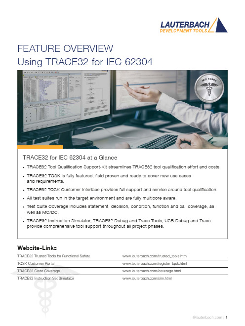
FEATURE OVERVIEWUsing TRACE32 for IEC 62304TRACE32 for IEC 62304 at a Glance• TRACE32 Tool Qualification Support-Kit streamlines TRACE32 tool qualification effort and costs.• TRACE32 TQSK is fully featured, field proven and ready to cover new use casesand requirements.• TRACE32 TQSK Customer Interface provides full support and service around tool qualification.• All test suites run in the target environment and are fully multicore aware.• Test Suite Coverage includes statement, decision, condition, function and call coverage, as well as MC/DC.• TRACE32 Instruction Simulator, TRACE32 Debug and Trace Tools, USB Debug and Trace provide comprehensive tool support throughout all project phases.Website-LinksTRACE32 Trusted Tools for Functional Safety /trusted_tools.htmlTQSK Customer Portal /register_tqsk.htmlTRACE32 Code Coverage /coverage.htmlTRACE32 Instruction Set Simulator /sim.htmlThe TRACE32 Tool Qualification Support-Kit (TQSK) provides everything needed to qualify use in safety-related software projects.Figure 1: The 2-stage qualification processCertification ArtifactsDocumentsTest SuiteTool Verification and Validation Supplement for Integration toOperational EnvironmentTest Suite DocumentsTest ReportTesting in Operational EnvironmentTest Report Testing inTSSTCTest Suite Simulator TriCore(paid)DSMDeveloper SafetyManualTSCTest Suite Coverage(free)TSDTest Suite Debug(free)$$TSSATest Suite Simulator Arm(paid)Test Suite SimulatorUpon customer request, Lauterbach also provides test suites for its Arm and TriCore Instruction Set Simulators. A qualified instruction set simulator is an accepted test environment in the software module testing phase of the project (see also figure 3) and offers the following advantages:• Product software qualification can start before product hardware is available.• The qualification of the product software can be well organized even in a distributed team, becauseeverything necessary is purely software-based.• If bottlenecks occur during this phase due to a lack of development hardware or debug/trace tools, additional test benches can be easily equipped with simulators.Test Suite DebugThe Test Suite Debug includes all basic debugging functionality such as target configuration, programming onchip and NOR flashes, loading programs, setting breakpoints and reading/writing of memory and variables.Figure 3: TRACE32 tool use in code coverage qualification。
- 1、下载文档前请自行甄别文档内容的完整性,平台不提供额外的编辑、内容补充、找答案等附加服务。
- 2、"仅部分预览"的文档,不可在线预览部分如存在完整性等问题,可反馈申请退款(可完整预览的文档不适用该条件!)。
- 3、如文档侵犯您的权益,请联系客服反馈,我们会尽快为您处理(人工客服工作时间:9:00-18:30)。
打开后的程序列表窗口可以有下面几种形式。 Pic24. 找不到源文件的程序列表窗口
对于上图所示的情形,需要用 Y.SPATH 命令指定源程序路径。如下图所示。 Pic25. 指定源程序路径(其一) Pic26. 带源程序的混合显示程序列表窗口(其二)
通过点击程序列表窗口上的“Mode”按钮可以切换混合和源码显示方式。 Pic27. 带源程序的源码程序列表窗口(其三)
这些设置主要包括: 1、 选择要调试的处理器型号。 2、 是否有多个器件串联在同一个 JTAG 链路里,连接顺序如何,每个器件的 JTAG IR
寄存器的宽度是多少。 (情况一) 3、 JTAG 时钟使用 TCK 还是 RTCK。TCK 由 TRACE-ICP 提供,一般情况下选用
10MHz。RTCK 是 TRACE-ICP 的 TCK 进入目标 JTAG 链路之后,从目标 JTAG 链路返回的时钟,它与目标处理器的时钟同步。一般情况下,具有睡眠模式的处理 器多选用 RTCK 作 JTAG 时钟, 如 ARM926EJ-S。 (情况二) 4、 通过 JTAG 与目标连接时,是否要先复位目标板。JTAG 口上的 SRST 信号产生复 位信号。 (情况三) 5、 通过 JTAG 与目标连接时,是否要停止目标处理器运行。 (情况四) 从主菜单“CPU”中选择“System Settings…” ,打开如下图所示对话框。从“CPU” 下拉菜单里选择要调试的处理器。 Pic2. System Settings 对话框
Pic29 中红框内的单选钮 IMASKASM 和 IMASKHLL 选择之后,单步时就会屏蔽中断。 用户也可以通过命令 sys.o imaskasm on 和 sys.o imaskhll on 来设置这两个选项。
十、 设置软件断点 设置软件断点可以在命令行输入命令 break.set <address> /soft 来实现,在命令中的 <address>代表程序地址,可以是程序中的函数名等符号。如下图所示。 Pic30. 用命令设置软件断点
五、 观察/修改存储器 从主菜单区点击“View->Dump…” ,打开存储器观察窗口,如下图所示。 Pic17. 存储器地址输入框
在地址输入框中输入要观察的地址,地址也可以用符号方式输入。输入地址之后点击 “OK”按钮,打开存储器显示窗口,如下图所示。 Pic18. 存储器显示窗口
用鼠标双击某一个存储单元的内容,在命令行就会出现存储器数据修改命令提示,用户 只要填入要修改的数据回车即可。如下图所示。 Pic19. 存储器修改命令提示
Trace32 软件使用
(亦可见 TRACE32-使用.pdf 与 icd_tutorial.pdf)
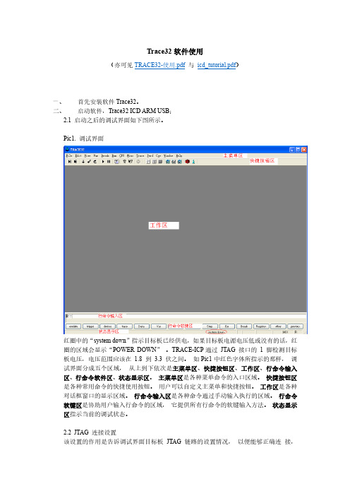
一、 首先安装软件 Trace32。 二、 启动软件,Trace32 ICD ARM USc1. 调试界面
红圈中的“system down”指示目标板已经供电,如果目标板电源电压低或没有的话,红 圈的区域会显示“POWER DOWN” 。TRACE-ICP 通过 JTAG 接口的 1 脚检测目标 板电压,电压范围应该在 1.8 到 3.3 伏之间。 如 Pic1 中红色字体所指示的那样, 调 试界面分成五个区域, 从上到下依次是主菜单区、快捷按钮区、工作区、行命令输入 区、行命令软件区、状态显示区。 主菜单区是各种菜单命令的入口区域。 快捷按钮区 是各种常用命令的快捷使用按钮。 用户可以自定义主菜单和快捷按钮。 工作区是各种 对话框窗口的显示区域。 行命令输入区是各种命令通过手动输入执行的区域。 行命令 软键区是协助用户输入行命令的区域, 它提供所有行命令的软键输入方法。 状态显示 区指示当前的调试状态。 2.2 JTAG 连接设置 该设置的作用是告诉调试界面目标板 JTAG 链路的设置情况, 以便能够正确连 接,
也可以通过在程序列表窗口的程序指令或源码旁边的空白处双击鼠标左键, 直 接在看到的程序上设置软件断点。如下图所示。 Pic31. 在程序列表窗口中设置软件断点
在 Pic31 中红色圆圈中的标示就是断点标示。另外,用户还可以在程序列表窗口中点击 鼠标右键,打开辅助对话框,选择 Breakpoints->Program。如下图所示。 Pic32. 通过鼠标右键设置软件断点
对于前面描述的第一种情况,多个器件串联在同一个 JTAG 链上,用户需要在图二十 三所示的对话框中选择“MultiCore” ,打开 MultiCore 对话窗口,如下图所示。 Pic3. MultiCore 对话框
最上方的红框中的部分描述多个器件在一个 JTAG 链上的位置。所谓“JTAG 串联” , 就是一个器件的 TDI 和另一个器件的 TDO 相连,没有连接的 TDI 与 JTAG 口的 TDI 连接,没有连接的 TDO 与 JTAG 口的 TDO 连接。图二十四中的红框中的图形 形象地描述了这种连接。在图形中, “core”表示被调试的处理器,如 ARM926EJ-S, “IRPOST”表示连接在 JTAG TDI 和“core”的 TDI 之间的器件的 JTAG IR 寄存器 长度的和,在“IRPOST”下方的编辑框内要填入这个和的值, “DRPOST”表示连接 在 JTAG TDI 和“core”的 TDI 之间的器件的数目,在“DRPOST”下方的编辑框内 填入这个数目值,“IRPRE”表示连接在 JTAG TDO 和“core”的 TDO 之间的器件的 JTAG IR 寄存器长度的和,在“IRPRE”下方的编辑框内要填入这个和的值,“DRPRE” 表示连接在 JTAG TDO 和“core”的 TDO 之间的器件的数目,在“DRPRE”下方的 编辑框内填入这个数目值。填入上面四个值,就完成了 JTAG MultCore 的设置。
如果选择“Attach”按钮并且目标处理器正在运行的话,在界面的状态显示区会有一个 绿色的“Running”条显示,如下图所示。
Pic8. Attach 连接成功
可以通过点击红圈中的按钮停止程序执行, 以便观察程序当前的处理器执行状态。 三、 运行脚本文件
从主菜单区点击“File->Run Batchfile…”打开脚本文件选择对话框。如下图所视。 Pic9. 脚本文件执行菜单
对前面描述的第二种情况,JTAG 时钟的选择,可以通过 System Settings 对话框上的 JtagClock 列表框来实现,如下图所示。
Pic4. JtagClock 列表框
红框中的部分就是 JtagClock 列表框,通过这个列表框用户可以选择 JTAG 时钟是 TCK 或 RTCK,选择 TCK 的时候,顺便选择它的频率,5MHz 或 10MHz 或 25MHz,也可以 手动在编辑框中输入频率值,如 1MHz。
如果在设置软件断点之前执行了 map.bonchip <range>命令, 并且所设置的软件断点在
<range>所指的地址范围内,那么,通过双击鼠标左键和单击鼠标右键设置软件断点的 方法所设置的断点将是 onchip 硬件断点。如果用户在 CPU 不能进行正确写操作的地 址上设置软件断点,将会出现下图所示的错误提示。 Pic33. 软件断点错误提示
符号表对话框如下图所示。 Pic22. 符号表对话框
在符号表对话框中可以通过单选钮“Symbols”选择要观察函数或是变量等符号。 在符 号表对话框中双击变量符号会打开变量观察对话框, 双击函数名会打开程序列表窗口。
八、 打开程序列表窗口 点击“View->List Source”打开程序列表窗口,如下图所示。 Pic23. 打开程序列表窗口
从主菜单区点击“CPU->Peripherals” ,打开设备寄存器窗口,如下图所示。 Pic14. 设备寄存器观察菜单
Pic15. 设备寄存器窗口
如上图所示的设备寄存器窗口在调试不同的处理器时是不同的。 如果用户要修改某个 寄存器的值, 双击该寄存器的值, 在行命令输入区就会出现相应的设备寄存器修改命 令,在命令后面输入要修改的值回车即可。如下图所示。 Pic16. 设备寄存器修改命令
对前面描述的第三种情况,通过 JTAG 与目标连接时,是否要先复位目标板,用户可以 通过下图中红框中的单选按钮进行选择。
Pic5. 系统复位选择
红框中的“EnReset”单选钮如果在前面打勾(选择),表示在 TRACE-ICP 做 JTAG 连 接时会做系统复位。 通过前面三种情况,用户完成了在 JTAG 连接动作之前的设置工作。接下来,用户就 可以连接目标了。这个连接通过下图中的红框中的“Up”或“Attach”单选钮来完成。 Pic6. JTAG 连接
Pic10. 脚本文件选择对话框
在图三十一所示的对话框中选择要执行的脚本文件,用户可以选择任意目录下的脚本文 件。脚本文件的内容主要以调试命令为主。有关脚本文件的编写,请参考软件安装目录 的“pdf”目录下的文件“practice_user.pdf”。脚本文件的 一般功能是自动执行 JTAG 设 置、目标处理器设备寄存器设置、下载要调试的应用程序(支持直接写入 FLASH)、设
选择红框中的“Up”单选钮,JTAG 通讯连接之后,目标处理器会停止执行,选择红框 中的“Attach”单选钮,JTAG 通讯连接之后,目标处理器处于它在 JTAG 通讯之前的 状态,原来是运行的,那么,它现在仍然保持运行状态,这就是我们前面描述的第四种 情况,如果用户在选择“Up”或“Attach”单选钮之后,在“Up”前面的小园框中有一 个绿色圆点,表明 JTAG 通讯已经连接成功。如下图所示。 Pic7. UP 连接成功
六、 下载程序 使用 data.load 命令实现程序下载的功能,如下图所示。 Pic20. 下载程序 上图中,“elf”指示所下载的程序的文件格式,“/v”指示程序下载完成之后进行校验。
七、 观察符号表 如下图所示,点击“View->Symbols->Browse”打开符号表对话框。 Pic21. 打开符号表对话框