信号与系统课后matlab作业.
信号与系统matlab实验及答案
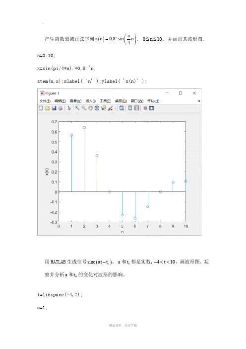
产生离散衰减正弦序列()π0.8sin 4n x n n ⎛⎫= ⎪⎝⎭, 010n ≤≤,并画出其波形图。
n=0:10;x=sin(pi/4*n).*0.8.^n;stem(n,x);xlabel( 'n' );ylabel( 'x(n)' );用MATLAB 生成信号()0sinc at t -, a 和0t 都是实数,410t -<<,画波形图。
观察并分析a 和0t 的变化对波形的影响。
t=linspace(-4,7); a=1;t0=2;y=sinc(a*t-t0); plot(t,y);t=linspace(-4,7); a=2;t0=2;y=sinc(a*t-t0); plot(t,y);t=linspace(-4,7); a=1;t0=2;y=sinc(a*t-t0); plot(t,y);三组对比可得a 越大最大值越小,t0越大图像对称轴越往右移某频率为f 的正弦波可表示为()()cos 2πa x t ft =,对其进行等间隔抽样,得到的离散样值序列可表示为()()a t nT x n x t ==,其中T 称为抽样间隔,代表相邻样值间的时间间隔,1s f T=表示抽样频率,即单位时间内抽取样值的个数。
抽样频率取40 Hz s f =,信号频率f 分别取5Hz, 10Hz, 20Hz 和30Hz 。
请在同一张图中同时画出连续信号()a x t t 和序列()x n nT 的波形图,并观察和对比分析样值序列的变化。
可能用到的函数为plot, stem, hold on 。
fs = 40;t = 0 : 1/fs : 1 ;% ƵÂÊ·Ö±ðΪ5Hz,10Hz,20Hz,30Hz f1=5;xa = cos(2*pi*f1*t) ; subplot(1, 2, 1) ;plot(t, xa) ;axis([0, max(t), min(xa), max(xa)]) ;xlabel('t(s)') ;ylabel('Xa(t)') ;line([0, max(t)],[0,0]) ; subplot(1, 2, 2) ;stem(t, xa, '.') ;line([0, max(t)], [0, 0]) ;axis([0, max(t), min(xa), max(xa)]) ;xlabel('n') ;ylabel('X(n)') ;频率越高,图像更加密集。
东南大学信号与系统MATLAB实践第三次作业
练习三实验三五.1.>>help windowWINDOW Window function gateway.WINDOW(@WNAME,N) returns an N-point window of type specifiedby the function handle @WNAME in a column vector. @WNAME canbe any valid window function name, for example:@bartlett - Bartlett window.@barthannwin - Modified Bartlett-Hanning window.@blackman - Blackman window.@blackmanharris - Minimum 4-term Blackman-Harris window.@bohmanwin - Bohman window.@chebwin - Chebyshev window.@flattopwin - Flat Top window.@gausswin - Gaussian window.@hamming - Hamming window.@hann - Hann window.@kaiser - Kaiser window.@nuttallwin - Nuttall defined minimum 4-term Blackman-Harris window.@parzenwin - Parzen (de la Valle-Poussin) window.@rectwin - Rectangular window.@tukeywin - Tukey window.@triang - Triangular window.WINDOW(@WNAME,N,OPT) designs the window with the optional input argument specified in OPT. To see what the optional input arguments are, see the helpfor the individual windows, for example, KAISER or CHEBWIN.WINDOW launches the Window Design & Analysis Tool (WinTool).EXAMPLE:N = 65;w = window(@blackmanharris,N);w1 = window(@hamming,N);w2 = window(@gausswin,N,2.5);plot(1:N,[w,w1,w2]); axis([1 N 0 1]);legend('Blackman-Harris','Hamming','Gaussian');See also bartlett, barthannwin, blackman, blackmanharris, bohmanwin,chebwin, gausswin, hamming, hann, kaiser, nuttallwin, parzenwin,rectwin, triang, tukeywin, wintool.Overloaded functions or methods (ones with the same name in other directories) help fdesign/window.mReference page in Help browser doc window 2.>>N = 128;w = window(@rectwin,N); w1 = window(@bartlett,N); w2 = window(@hamming,N);plot(1:N,[w,w1,w2]); axis([1 N 0 1]); legend('矩形窗','Bartlett','Hamming');2040608010012000.10.20.30.40.50.60.70.80.913.>>wvtool(w,w1,w2)六.ts=0.01;N=20;t=0:ts:(N-1)*ts;x=2*sin(4*pi*t)+5*cos(6*pi*t);g=fft(x,N);y=abs(g)/100;figure(1):plot(0:2*pi/N:2*pi*(N-1)/N,y); grid;01234560.050.10.150.20.250.30.350.40.45ts=0.01; N=30;t=0:ts:(N-1)*ts;x=2*sin(4*pi*t)+5*cos(6*pi*t); g=fft(x,N); y=abs(g)/100;figure(2):plot(0:2*pi/N:2*pi*(N-1)/N,y); grid;012345670.10.20.30.40.50.60.7ts=0.01; N=50;t=0:ts:(N-1)*ts;x=2*sin(4*pi*t)+5*cos(6*pi*t); g=fft(x,N); y=abs(g)/100;figure(3):plot(0:2*pi/N:2*pi*(N-1)/N,y); grid;123456700.10.20.30.40.50.60.70.80.91ts=0.01; N=100;t=0:ts:(N-1)*ts;x=2*sin(4*pi*t)+5*cos(6*pi*t); g=fft(x,N); y=abs(g)/100;figure(4):plot(0:2*pi/N:2*pi*(N-1)/N,y); grid;012345670.511.522.5ts=0.01; N=150;t=0:ts:(N-1)*ts;x=2*sin(4*pi*t)+5*cos(6*pi*t); g=fft(x,N); y=abs(g)/100;figure(5):plot(0:2*pi/N:2*pi*(N-1)/N,y); grid;012345670.511.522.53实验八 1.%冲激响应 >> clear; b=[1,3]; a=[1,3,2]; sys=tf(b,a); impulse(sys); 结果:Impulse ResponseTime (sec)A m p l i t u d e%求零输入响应 >> A=[1,3;0,-2]; B=[1;2]; Q=A\B Q = 4-1>> clear B=[1,3]; A=[1,3,2];[a,b,c,d]=tf2ss(B,A) sys=ss(a,b,c,d); x0=[4;-1]; initial(sys,x0); grid; a =-3 -2 1 0 b =1 0 c =1 3 d = 001234560.20.40.60.811.21.4Response to Initial ConditionsTime (sec)A m p l i t u d e2.%冲激响应 >> clear; b=[1,3]; a=[1,2,2]; sys=tf(b,a); impulse(sys)Impulse ResponseTime (sec)A m p l i t u d e%求零输入响应 >> A=[1,3;1,-2]; B=[1;2]; Q=A\B Q =1.6000 -0.2000 >> clear B=[1,3]; A=[1,2,2];[a,b,c,d]=tf2ss(B,A) sys=ss(a,b,c,d); x0=[1.6;-0.2]; initial(sys,x0); grid; a =-2 -2 1 0 b = 10 c =1 3 d = 0Response to Initial ConditionsTime (sec)A m p l i t u d e3.%冲激响应 >> clear; b=[1,3]; a=[1,2,1]; sys=tf(b,a); impulse(sys)Impulse ResponseTime (sec)A m p l i t u d e%求零输入响应 >> A=[1,3;1,-1]; B=[1;2]; Q=A\B Q =1.7500 -0.2500>> clear B=[1,3]; A=[1,2,1];[a,b,c,d]=tf2ss(B,A) sys=ss(a,b,c,d); x0=[1.75;-0.25]; initial(sys,x0); grid; a =-2 -1 1 0 b =1 0 c =1 3 d = 00510150.20.40.60.811.21.41.6Response to Initial ConditionsTime (sec)A m p l i t u d e二. >> clear; b=1;a=[1,1,1,0]; sys=tf(b,a); subplot(2,1,1);impulse(sys);title('冲击响应'); subplot(2,1,2);step(sys);title('阶跃响应'); t=0:0.01:20; e=sin(t);r=lsim(sys,e,t); figure;subplot(2,1,1);plot(t,e);xlabel('Time');ylabel('A');title('激励信号'); subplot(2,1,2);plot(t,r);xlabel('Time');ylabel('A');title('响应信号');024681012141618200.511.5冲击响应Time (sec)A m p l i t u d e024681012141618205101520阶跃响应Time (sec)A m p l i t u d e02468101214161820-1-0.500.51Time A激励信号2468101214161820-10123TimeA响应信号三. 1.>> clear; b=[1,3]; a=[1,3,2]; t=0:0.08:8; e=[exp(-3*t)]; sys=tf(b,a); lsim(sys,e,t);0.10.20.30.40.50.60.70.80.91Linear Simulation ResultsTime (sec)A m p l i t u d e2.>> clear; b=[1,3]; a=[1,2,2]; t=0:0.08:8; sys=tf(b,a); step(sys)0.20.40.60.811.21.41.6Step ResponseTime (sec)A m p l i t u d e3.>> clear; b=[1,3]; a=[1,2,1]; t=0:0.08:8; e=[exp(-2*t)]; sys=tf(b,a); lsim(sys,e,t);0.10.20.30.40.50.60.70.80.91Linear Simulation ResultsTime (sec)A m p l i t u d eDoc: 1.>> clear; B=[1]; A=[1,1,1]; sys=tf(B,A,-1); n=0:200;e=5+cos(0.2*pi*n)+2*sin(0.7*pi*n); r=lsim(sys,e); stem(n,r);0204060801001201401601802002.>> clear;B=[1,1,1];A=[1,-0.5,-0.5];sys=tf(B,A,-1);e=[1,zeros(1,100)];n=0:100;r=lsim(sys,e);stem(n,r);010203040506070809010021 / 21。
长江大学信号与系统matlab实验答案
实验1 信号变换与系统非时变性质的波形绘制●用MA TLAB画出习题1-8的波形。
●用MA TLAB画出习题1-10的波形。
Eg 1.8代码如下:function [y]=zdyt(t) %定义函数zdyty=-2/3*(t-3).*(heaviside(-t+3)-heaviside(-t));endt0=-10;t1=4;dt=0.02;t=t0:dt:t1;f=zdyt(t);y=zdyt(t+3);x=zdyt(2*t-2);g=zdyt(2-2*t);h=zdyt(-0.5*t-1);fe=0.5*(zdyt(t)+zdyt(-t));fo=0.5*(zdyt(t)-zdyt(-t));subplot(7,1,1),plot(t,f);title('信号波形的变化')ylabel('f(t)')grid;line([t0 t1],[0 0]);subplot(7,1,2),plot(t,y);ylabel('y(t)')grid;line([t0 t1],[0 0]);subplot(7,1,3),plot(t,x);ylabel('x(t)')grid;line([t0 t1],[0 0]);subplot(7,1,4),plot(t,g);ylabel('g(t)')grid;line([t0 t1],[0 0]);subplot(7,1,5),plot(t,h);ylabel('h(t)')grid;line([t0 t1],[0 0]);subplot(7,1,6),plot(t,fe);ylabel('fe(t)')grid;line([t0 t1],[0 0]);subplot(7,1,7),plot(t,fo);ylabel('fo(t)')grid;line([t0 t1],[0 0]);xlabel('Time(sec)')结果:Eg1.10代码如下:function [u]=f(t) %定义函数f(t) u= heaviside(t)-heaviside(t-2); endfunction [u] =y(t) %定义函数y(t)u=2*(t.*heaviside(t)-2*(t-1).*heaviside(t-1)+(t-2).*heaviside(t-2)); endt0=-2;t1=5;dt=0.01; t=t0:dt:t1; f1=f(t); y1=y(t); f2=f(t)-f(t-2); y2=y(t)-y(t-2); f3=f(t)-f(t+1); y3=y(t)-y(t+1);subplot(3,2,1),plot(t,f1); title('激励——响应波形图') ylabel('f1(t)')grid;line([t0 t1],[0 0]);-10-8-6-4-2024012信号波形的变化f (t)-10-8-6-4-2024012y (t)-10-8-6-4-2024012x (t)-10-8-6-4-2024012g (t)-10-8-6-4-2024012h (t)-10-8-6-4-202400.51f e (t)-10-8-6-4-2024-101f o (t)Time(sec)subplot(3,2,2),plot(t,y1); ylabel('y1(t)')grid;line([t0 t1],[0 0]); subplot(3,2,3),plot(t,f2); ylabel('f2(t)')grid;line([t0 t1],[0 0]); subplot(3,2,4),plot(t,y2); ylabel('y2(t)')grid;line([t0 t1],[0 0]); subplot(3,2,5),plot(t,f3); ylabel('f3(t)')grid;line([t0 t1],[0 0]); subplot(3,2,6),plot(t,y3); ylabel('y3(t)')grid;line([t0 t1],[0 0]); xlabel('Time(sec)')结果:实验2 微分方程的符号计算和波形绘制上机内容用MA TLAB 计算习题2-1,并画出系统响应的波形。
信号与系统课后matlab作业
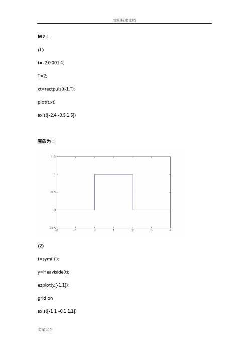
(1)t=-2:0.001:4;T=2;xt=rectpuls(t-1,T); plot(t,xt)axis([-2,4,-0.5,1.5]) 图象为:(2)t=sym('t');y=Heaviside(t); ezplot(y,[-1,1]); grid onaxis([-1 1 -0.1 1.1])(3)A=10;a=-1;B=5;b=-2;t=0:0.001:10;xt=A*exp(a*t)-B*exp(b*t); plot(t,xt)图象为:(4)y=t*Heaviside(t); ezplot(y,[-1,3]);grid onaxis([-1 3 -0.1 3.1])图象为:(5)A=2;w0=10*pi;phi=pi/6; t=0:0.001:0.5;xt=abs(A*sin(w0*t+phi)); plot(t,xt)图象为:(6)A=1;w0=1;B=1;w1=2*pi;t=0:0.001:20;xt=A*cos(w0*t)+B*sin(w1*t); plot(t,xt)图象为:(7)A=4;a=-0.5;w0=2*pi;t=0:0.001:10;xt=A*exp(a*t).*cos(w0*t); plot(t,xt)图象为:(8)w0=30;t=-15:0.001:15;xt=cos(w0*t).*sinc(t/pi); plot(t,xt)axis([-15,15,-1.1,1.1])图象为:M2-3(1)function yt=x2_3(t)yt=(t).*(t>=0&t<=2)+2*(t>=2&t<=3)-1*(t>=3&t<=5); (2)function yt=x2_3(t)yt=(t).*(t>=0&t<=2)+2*(t>=2&t<=3)-1*(t>=3&t<=5);t=0:0.001:6;subplot(3,1,1)plot(t,x2_3(t))title('x(t)')axis([0,6,-2,3])subplot(3,1,2)plot(t,x2_3(0.5*t))title('x(0.5t)')axis([0,11,-2,3])subplot(3,1,3)plot(t,x2_3(2-0.5*t))title('x(2-0.5t)')axis([-6,5,-2,3])图像为:M2-9(1)k=-4:7;xk=[-3,-2,3,1,-2,-3,-4,2,-1,4,1,-1];stem(k,xk,'file')(2)k=-12:21;x=[-3,0,0,-2,0,0,3,0,0,1,0,0,-2,0,0,-3,0,0,-4,0,0,2,0,0,-1,0,0,4,0,0,1,0,0,-1]; subplot(2,1,1)stem(k,x,'file')title('3倍内插')t=-1:2;y=[-2,-2,2,1];subplot(2,1,2)stem(t,y,'file')title('3倍抽取')axis([-3,4,-4,4])(3)k=-4:7;x=[-3,-2,3,1,-2,-3,-4,2,-1,4,1,-1]; subplot(2,1,1)stem(k+2,x,'file')title('x[k+2]')subplot(2,1,2)stem(k-4,x,'file')title('x[k-4]')(4)k=-4:7;x=[-3,-2,3,1,-2,-3,-4,2,-1,4,1,-1]; stem(-fliplr(k),fliplr(x),'file') title('x[-k]')M3-1(1)ts=0;te=5;dt=0.01; sys=tf([2 1],[1 3 2]); t=ts:dt:te;x=exp(-3*t);y=lsim(sys,x,t); plot(t,y)xlabel('Time(sec)') ylabel('y(t)')(2)ts=0;te=5;dt=1; sys=tf([2 1],[1 3 2]); t=ts:dt:te;x=exp(-3*t);y=lsim(sys,x,t)y =0.6649-0.0239-0.0630-0.0314-0.0127从(1)(2)对比我们当抽样间隔越小时数值精度越高。
东南大学信号与系统MATLAB实践第二次作业
东南大学信号与系统MATLAB实践第二次作业. . . . 练习二实验六一.用MATLAB语言描述下列系统,并求出极零点、1.>> Ns=[1];Ds=[1,1];sys1=tf(Ns,Ds)实验结果:sys1 =1-----s + 1>> [z,p,k]=tf2zp([1],[1,1])z =Empty matrix: 0-by-1p =. . . .-1k =12.>>Ns=[10]Ds=[1,-5,0]sys2=tf(Ns,Ds)实验结果:Ns =10Ds =sys2 =10---------s^2 - 5 s>>[z,p,k]=tf2zp([10],[1,-5,0]) z =Empty matrix: 0-by-1p =5k =10二.已知系统的系统函数如下,用MATLAB描述下列系统。
1.>> z=[0];p=[-1,-4];k=1;sys1=zpk(z,p,k)实验结果:sys1 =s-----------(s+1) (s+4)Continuous-time zero/pole/gain model.2.>> Ns=[1,1]Ds=[1,0,-1]sys2=tf(Ns,Ds)实验结果:Ns =1 1Ds =sys2 =s + 1-------s^2 - 1Continuous-time transfer function.3.>> Ns=[1,6,6,0];Ds=[1,6,8];sys3=tf(Ns,Ds)实验结果:Ns =1 6 6 0Ds =1 6 8sys3 =s^3 + 6 s^2 + 6 s-----------------s^2 + 6 s + 8Continuous-time transfer function.六.已知下列H(s)或H(z),请分别画出其直角坐标系下的频率特性曲线。
1.>> clear;for n = 1:400w(n) = (n-1)*0.05;H(n) = (1j*w(n))/(1j*w(n)+1); endmag = abs(H);phase = angle(H);subplot(2,1,1)plot(w,mag);title('幅频特性') subplot(2,1,2)plot(w,phase);title('相频特性')实验结果:2.>> clear;for n = 1:400w(n) = (n-1)*0.05;H(n) = (2*j*w(n))/((1j*w(n))^2+sqrt(2)*j*w(n)+1); end mag = abs(H);phase = angle(H);subplot(2,1,1)plot(w,mag);title('幅频特性')subplot(2,1,2)plot(w,phase);title('相频特性')实验结果:3.>>clear;for n = 1:400w(n) = (n-1)*0.05;H(n) = (1j*w(n)+1)^2/((1j*w(n))^2+0.61); end mag = abs(H);phase = angle(H);subplot(2,1,1)plot(w,mag);title('幅频特性')subplot(2,1,2)plot(w,phase);title('相频特性')实验结果:4.>>clear;for n = 1:400w(n) = (n-1)*0.05;H(n) =3*(1j*w(n)-1)*(1j*w(n)-2)/(1j*w(n)+1)*(1j*w(n)+2); end mag = abs(H);phase = angle(H);subplot(2,1,1)plot(w,mag);title('幅频特性')subplot(2,1,2)plot(w,phase);title('相频特性') 实验结果:实验七三.已知下列传递函数H(s)或H(z),求其极零点,并画出极零图。
信号与系统matlab课后作业-北京交通大学
信号与系统MATLAB平时作业学院:电子信息工程学院班级::学号:教师:钱满义MATLAB 习题M3-1 一个连续时间LTI系统满足的微分方程为y ’’(t)+3y ’(t)+2y(t)=2x ’(t)+x(t)(1)已知x(t)=e -3t u(t),试求该系统的零状态响应y zs (t); (2)用lism 求出该系统的零状态响应的数值解。
利用(1)所求得的结果,比较不同的抽样间隔对数值解精度的影响。
解:(1) 由于''()3'()2()2'()(),0h t h t h t t t t δδ++=+≥则2()()()t t h t Ae Be u t --=+ 将()h t 带入原方程式化简得(2)()()'()2'()()A B t A B t t t δδδδ+++=+所以1,3A B =-=2()(3)()t t h t e e u t --=-+又因为3t ()()x t e u t -= 则该系统的零状态响应3t 23t 2t ()()()()(3)()0.5(6+5)()zs t t t y t x t h t e u t e e u t e e e u t ----=*=*-+=-- (2)程序代码 1、ts=0;te=5;dt=0.1;sys=tf([2 1],[1 3 2]);t=ts:dt:te;x=exp(-3*t).*(t>=0);y=lsim(sys,x,t)2、ts=0;te=5;dt=1;sys=tf([2 1],[1 3 2]);t=ts:dt:te;x=exp(-3*t).*(t>=0);y1=-0.5*exp(-3*t).*(exp(2*t)-6*exp(t)+5).*[t>=0];y2=lsim(sys,x,t)plot(t,y1,'r-',t,y2,'b--')xlabel('Time(sec)')legend('实际值','数值解')用lism求出的该系统的零状态响应的数值解在不同的抽样间隔时与(1)中求出的实际值进行比较将两种结果画在同一幅图中有图表 1 抽样间隔为1图表 2 抽样间隔为0.1图表 3 抽样间隔为0.01当抽样间隔dt减小时,数值解的精度越来越高,从图像上也可以看出数值解曲线越来越逼近实际值曲线,直至几乎重合。
信号与系统matlab实验习题3 绘制典型信号及其频谱图
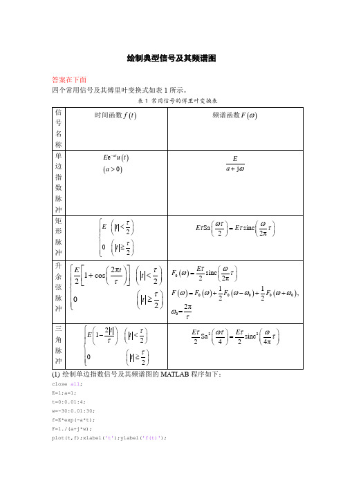
绘制典型信号及其频谱图答案在下面四个常用信号及其傅里叶变换式如表1所示。
(1)绘制单边指数信号及其频谱图的MATLAB程序如下:close all;E=1;a=1;t=0:0.01:4;w=-30:0.01:30;f=E*exp(-a*t);F=1./(a+j*w);plot(t,f);xlabel('t');ylabel('f(t)');figure;plot(w,abs(F));xlabel('\omega');ylabel('|F(\omega)|');figure;max_logF=max(abs(F));plot(w,20*log10(abs(F)/max_logF));xlabel('\omega');ylabel('|F(\omega)| indB');figure;plot(w,angle(F));xlabel('\omega');ylabel('\phi(\omega)');请更改参数,调试此程序,绘制单边指数信号的波形图和频谱图。
观察参数a 对信号波形及其频谱的影响。
注:题目中阴影部分是幅频特性的对数表示形式,单位是(dB),请查阅相关资料,了解这种表示方法的意义及其典型数值对应的线性增益大小。
(2)绘制矩形脉冲信号、升余弦脉冲信号和三角脉冲信号的波形图和频谱图,观察并对比各信号的频带宽度和旁瓣的大小。
(3)更改参数,调试程序,绘制单边指数信号的波形图和频谱图。
观察参数a对信号波形及其频谱的影响。
答案附上程序代码:close all;E=1;a=1;t=0:0.01:4;w=-30:0.01:30;f=E*exp(-a*t);F=1./(a+j*w);plot(t,f);xlabel('t');ylabel('f(t)');figure;plot(w,abs(F));xlabel('\omega');ylabel('|F(\omega)|';E=1,a=1,波形图 频谱图更改参数E=2,a=1;更改参数a ,对信号波形及其频谱的影响。
信号与系统课程作业
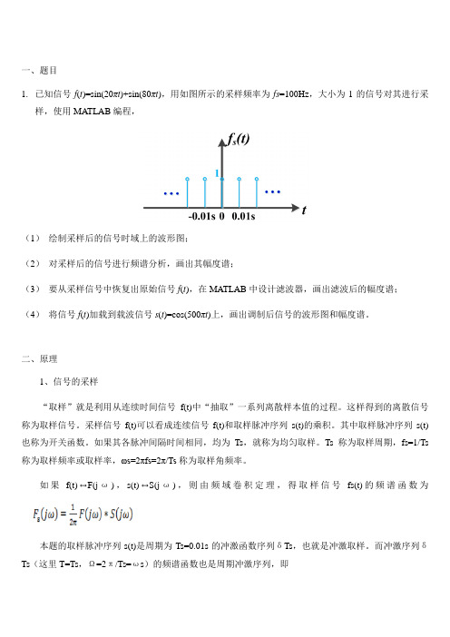
一、题目1.已知信号f(t)=sin(20πt)+sin(80πt),用如图所示的采样频率为fs=100Hz,大小为1的信号对其进行采样,使用MATLAB编程,(1)绘制采样后的信号时域上的波形图;(2)对采样后的信号进行频谱分析,画出其幅度谱;(3)要从采样信号中恢复出原始信号f(t),在MATLAB中设计滤波器,画出滤波后的幅度谱;(4)将信号f(t)加载到载波信号s(t)=cos(500πt)上,画出调制后信号的波形图和幅度谱。
二、原理1、信号的采样“取样”就是利用从连续时间信号f(t)中“抽取”一系列离散样本值的过程。
这样得到的离散信号称为取样信号。
采样信号f(t)可以看成连续信号f(t)和取样脉冲序列s(t)的乘积。
其中取样脉冲序列s(t)也称为开关函数。
如果其各脉冲间隔时间相同,均为Ts,就称为均匀取样。
Ts称为取样周期,fs=1/Ts 称为取样频率或取样率,ωs=2πfs=2π/Ts称为取样角频率。
如果f(t)↔F(jω),s(t)↔S(jω),则由频域卷积定理,得取样信号fs(t)的频谱函数为本题的取样脉冲序列s(t)是周期为Ts=0.01s的冲激函数序列δTs,也就是冲激取样。
而冲激序列δTs(这里T=Ts,Ω=2π/Ts=ωs)的频谱函数也是周期冲激序列,即2、采样定理所谓模拟信号的数字处理方法就是将待处理模拟信号经过采样、量化和编码形成数字信号,再利用数字信号处理技术对采样得到的数字信号进行处理。
一个频带限制在(0,fc)Hz的模拟信号m(t),若以采样频率fs≥2fc对模拟信号m(t)进行采样,得到最终的采样值,则可无混叠失真地恢复原始模拟信号m(t)。
其中,无混叠失真地恢复原始模拟信号m(t)是指被恢复信号与原始模拟信号在频谱上无混叠失真,并不是说被恢复信号与原始信号在时域上完全一样。
由于采样和恢复器件的精度限制以及量化误差等存在,两者实际是存在一定误差或失真的。
奈奎斯特频率:通常把最低允许的采样频率fs=2fc称为奈奎斯特频率。
- 1、下载文档前请自行甄别文档内容的完整性,平台不提供额外的编辑、内容补充、找答案等附加服务。
- 2、"仅部分预览"的文档,不可在线预览部分如存在完整性等问题,可反馈申请退款(可完整预览的文档不适用该条件!)。
- 3、如文档侵犯您的权益,请联系客服反馈,我们会尽快为您处理(人工客服工作时间:9:00-18:30)。
(1)t=-2:0.001:4;T=2;xt=rectpuls(t-1,T); plot(t,xt)axis([-2,4,-0.5,1.5]) 图象为:(2)t=sym('t');y=Heaviside(t); ezplot(y,[-1,1]); grid onaxis([-1 1 -0.1 1.1]) 图象为:A=10;a=-1;B=5;b=-2;t=0:0.001:10;xt=A*exp(a*t)-B*exp(b*t); plot(t,xt)图象为:(4)t=sym('t');y=t*Heaviside(t);ezplot(y,[-1,3]);grid onaxis([-1 3 -0.1 3.1])图象为:A=2;w0=10*pi;phi=pi/6;t=0:0.001:0.5;xt=abs(A*sin(w0*t+phi)); plot(t,xt)图象为:(6)A=1;w0=1;B=1;w1=2*pi;t=0:0.001:20;xt=A*cos(w0*t)+B*sin(w1*t); plot(t,xt)图象为:A=4;a=-0.5;w0=2*pi;t=0:0.001:10;xt=A*exp(a*t).*cos(w0*t); plot(t,xt)图象为:(8)w0=30;t=-15:0.001:15;xt=cos(w0*t).*sinc(t/pi); plot(t,xt)axis([-15,15,-1.1,1.1])图象为:(1)function yt=x2_3(t)yt=(t).*(t>=0&t<=2)+2*(t>=2&t<=3)-1*(t>=3&t<=5); (2)function yt=x2_3(t)yt=(t).*(t>=0&t<=2)+2*(t>=2&t<=3)-1*(t>=3&t<=5);t=0:0.001:6;subplot(3,1,1)plot(t,x2_3(t))title('x(t)')axis([0,6,-2,3])subplot(3,1,2)plot(t,x2_3(0.5*t))title('x(0.5t)')axis([0,11,-2,3])subplot(3,1,3)plot(t,x2_3(2-0.5*t))title('x(2-0.5t)')axis([-6,5,-2,3])图像为:M2-9(1)k=-4:7;xk=[-3,-2,3,1,-2,-3,-4,2,-1,4,1,-1];stem(k,xk,'file')(2)k=-12:21;x=[-3,0,0,-2,0,0,3,0,0,1,0,0,-2,0,0,-3,0,0,-4,0,0,2,0,0,-1,0,0,4,0,0,1,0,0,-1]; subplot(2,1,1)stem(k,x,'file')title('3倍内插')t=-1:2;y=[-2,-2,2,1];subplot(2,1,2)stem(t,y,'file')title('3倍抽取')axis([-3,4,-4,4])k=-4:7;x=[-3,-2,3,1,-2,-3,-4,2,-1,4,1,-1]; subplot(2,1,1)stem(k+2,x,'file')title('x[k+2]')subplot(2,1,2)stem(k-4,x,'file')title('x[k-4]')(4)k=-4:7;x=[-3,-2,3,1,-2,-3,-4,2,-1,4,1,-1]; stem(-fliplr(k),fliplr(x),'file') title('x[-k]')(1)ts=0;te=5;dt=0.01;sys=tf([2 1],[1 3 2]);t=ts:dt:te;x=exp(-3*t);y=lsim(sys,x,t);plot(t,y)xlabel('Time(sec)')ylabel('y(t)')(2)ts=0;te=5;dt=1;sys=tf([2 1],[1 3 2]);t=ts:dt:te;x=exp(-3*t);y=lsim(sys,x,t)y =0.6649-0.0239-0.0630-0.0314-0.0127从(1)(2)对比我们当抽样间隔越小时数值精度越高。
x=[0.85,0.53,0.21,0.67,0.84,0.12]; kx=-2:3;h=[0.68,0.37,0.83,0.52,0.71];kh=-1:3;y=conv(x,h);k=kx(1)+kh(1):kx(end)+kh(end); stem(k,y,'file');M3-8k=0:30;a=[1 0.7 -0.45 -0.6];b=[0.8 -0.44 0.36 0.02];h=impz(b,a,k);stem(k,h,'file')(1)对于周期矩形信号的傅里叶级数cn =-1/2j*sin(n/2*pi)*sinc(n/2) n=-15:15;X=-j*1/2*sin(n/2*pi).*sinc(n/2);subplot(2,1,1);stem(n,abs(X),'file');title('幅度谱')xlabel('nw');subplot(2,1,2);stem(n,angle(X),'file');title('相位谱')(2)对于三角波信号的频谱是:Cn=-++n=-15:15;X=sinc(n)-0.5*((sinc(n/2)).^2);subplot(2,1,1);stem(n,abs(X),'file');title('幅度谱')xlabel('nw');subplot(2,1,2);stem(n,angle(X),'file');title('相位谱')M4-6(4)x=[1,2,3,0,0];X=fft(x,5);subplot(2,1,1);m=0:4;stem(m,real(X),'file'); title('X[m]实部') subplot(2,1,2);stem(m,imag(X),'file'); title('X[m]虚部')M4-7(3)k=0:10;x=0.5.^k;subplot(3,1,1);stem(k,x,'file')title('x[k]')X=fft(x,10);subplot(3,1,2);m=0:9;stem(m,real(X),'file');title('X[m]实部')subplot(3,1,3);stem(m,imag(X),'file');title('X[m]虚部')M5-2t=0:0.05:2.5;T=1;xt1=rectpuls(t-0.5,T);subplot(2,2,1)plot(t,xt1)title('x(t1)')axis([0,2.5,0,2])xt2=tripuls(t-1,2);subplot(2,2,2)plot(t,xt2)title('x(t2)')axis([0,2.5,0,2])xt=xt1+xt2.*cos(50*t);subplot(2,2,[3,4])plot(t,xt)title('x(t)')figure;b=[10000];a=[1,26.131,341.42,2613.1,10000]; [H,w]=freqs(b,a,w);subplot(2,1,1)plot(w,abs(H));title('幅度曲线')subplot(2,1,2)plot(w,angle(H));title('相位曲线')figure;sys=tf([10000],[1 26.131 341.42 2613.1 10000]);yt1=lsim(sys,xt,t);subplot(2,1,1);plot(t,yt1);title('y(t1)')yt2=lsim(sys,xt.*cos(50*t),t);subplot(2,1,2);plot(t,yt2);title('y(t2)')M6-1(1)num=[41.6667];den=[1 3.7444 25.7604 41.6667];[r,p,k]=residue(num,den)r =-0.9361 - 0.1895i -0.9361 + 0.1895i 1.8722p =-0.9361 + 4.6237i -0.9361 - 4.6237i -1.8722k =[](2)num=[16 0 0];den=[1 5.6569 816 2262.7 160000];[r,p,k]=residue(num,den)r =0.0992 - 1.5147i 0.0992 + 1.5147i -0.0992 + 1.3137i -0.0992 - 1.3137ip =-1.5145 +21.4145i -1.5145 -21.4145i -1.3140 +18.5860i -1.3140 -18.5860i k =[](3)num=[1 0 0 0];den=conv([1 5],[1 5 25]);[r,p,k]=residue(num,den)r =-2.5000 - 1.4434i -2.5000 + 1.4434i -5.0000p =-2.5000 + 4.3301i -2.5000 - 4.3301i -5.0000k =1(4)num=[833.3025];den=conv([1 4.1123 28.867],[1 9.9279 28.867]);[r,p,k]=residue(num,den)r =-2.4819 + 1.0281i -2.4819 - 1.0281i 2.4819 - 5.9928i 2.4819 + 5.9928i p =-2.0562 + 4.9638i -2.0562 - 4.9638i -4.9640 + 2.0558i -4.9640 - 2.0558i k =[]M6-2sys=tf(b,a);x=1*(t>0)+0*(t<=0);y1=lsim(sys,x,t);plot(t,y1);title('零状态响应')figure;[A B C D]=tf2ss(b,a);sys=ss(A,B,C,D);x=1*(t>0)+0*(t<=0);zi=[1 2];y=lsim(sys,x,t,zi);plot(t,y);title('完全响应')figure;y2=y-y1;plot(t,y2);title('零输入响应')a=[1 2 2 1];b=[1 2];sys=tf(b,a); pzmap(sys)冲击响应a=[1 2 2 1];b=[1 2];sys=tf(b,a); impulse(sys)阶跃响应a=[1 2 2 1];b=[1 2];sys=tf(b,a);step(sys)频率响应a=[1 2 2 1];b=[1 2];w=linspace(-10,10,2 0000);H=freqs(b,a,w); plot(w,abs(H))(1)num=[2 16 44 56 32];den=[3 3 -15 18 -12];[r,p,k]=residuez(num,den)r =-0.0177 9.4914 -3.0702 + 2.3398i -3.0702 - 2.3398ip =-3.2361 1.2361 0.5000 + 0.8660i 0.5000 - 0.8660ik =-2.6667(2)num=[4 -8.86 -17.98 26.74 -8.04];den=[1 -2 10 6 65];[r,p,k]=residuez(num,den)r =1.0849 + 1.3745i 1.0849 - 1.3745i 0.9769 - 1.2503i 0.9769 + 1.2503i p =2.0000 + 3.0000i 2.0000 - 3.0000i -1.0000 + 2.0000i -1.0000 - 2.0000i k =-0.1237M7-2k=0:10;a=[2 -1 3];b=[2 -1];y1=filter(b,a,x);stem(k,y1)title('零状态响应')figure;h=impz(b,a,k);x=0.5.^k;y2=conv(x,h);N=length(y2);stem(0:N-1,y2)title('零输入响应')完全响应y=y1+y2(1)num=[2 16 44 56 32];den=[3 3 -15 18 -12];zplane(num,den)由图可知极点不是都在单位圆内,所以系统不是稳定系统。