实验二 MATLAB基础知识(二)
MATLAB实验答案(桂电)
实验一 MATLAB入门(1)1.实验目的:(1)了解MATLAB的体系结构与特点,熟悉其集成开发环境。
(2)熟悉MATLAB界面窗口的功能和使用方法。
(3)熟悉MATLAB的帮助系统及使用方法。
(4)了解MATLAB的的数据类型、基本形式和数组的产生方法。
(5)掌握MATLAB基本的数学运算操作。
2.实验原理(1)MATLAB简介MATLAB是美国MathWorks公司开发的高性能的科学与工程计算软件。
它在数值计算、自动控制、信号处理、神经网络、优化计算、小波分析、图像处理等领域有着广泛的用途。
近年来, MATLAB在国内高等院校、科研院所的应用逐渐普及,成为广大科研、工程技术人员必备的工具之一。
MATLAB具有矩阵和数组运算方便、编程效率极高、易学易用、可扩充性强和移植性好等优点,俗称为“草稿纸式的科学计算语言”。
它把工程技术人员从繁琐的程序代码编写工作中解放出来,可以快速地验证自己的模型和算法。
经过几十年的扩充和完善,MATLAB已经发展成为集科学计算、可视化和编程于一体的高性能的科学计算语言和软件开发环境,整套软件由MATLAB开发环境、MATLAB语言、MATLAB数学函数库、MATLAB图形处理系统和MATLAB应用程序接口(API)等五大部分组成。
MATLAB的主要特点包括强大的计算能力(尤其是矩阵计算能力)、方便的绘图功能及仿真能力、极高的编程效率。
另外,MATLAB还附带了大量的专用工具箱,用于解决各种特定领域的问题。
通过学习软件的基本操作及其编程方法,体会和逐步掌握它在矩阵运算、信号处理等方面的功能及其具体应用。
通过本课程实验的学习,要求学生初步掌握MATLAB的使用方法,初步掌握M文件的编写和运行方法,初步将MATLAB运用于数字信号处理中。
循序渐进地培养学生运用所学知识分析和解决问题的能力。
(2)MATLAB的工作界面(Desktop)与操作MATLAB 安装成功后,第一次启动时,主界面如下图(不同版本可能有差异)所示:其中① 是命令窗口(Command Window ),是MATLAB 的主窗口,默认位于MATLAB界面的右侧,用于输入命令、运行命令并显示运行结果。
实验二MATLAB绘制图形
grid on %在所画出的图形坐标中加入栅格
绘制图形如下
50
10
1
0.8
40
10
0.6
0.4
30
10
0.2
0
1020
-0.2
-0.4
1010
-0.6
-0.8
0
10
-1
-2
0
2
-2
0
2
10
10
10
10
10
10
如果在图中不加栅格
程序如下:
clear x=logspace(-1,2);%在10^(-1)到10^2之间产生50个 对数等分的行向量 subplot(121); loglog(x,10*exp(x),'-p') subplot(122); semilogx(x,cos(10.^x))
(2)plot(x,y): 基本格式,x和y可为向量或矩阵. 1. 如果x,y是同维向量,以x元素为横坐标,以y元素 为纵坐标绘图. 2. 如果x是向量,y是有一维与x元素数量相等的矩阵, 则以x为共同横坐标, y元素为纵坐标绘图,曲线数目 为y的另一维数. 3. 如果x,y是同维矩阵,则按列以x,y对应列元素为 横、纵坐标绘图,曲线数目等于矩阵列数.
y=2*exp(-0.5*x).*cos(4*pi*x);
2
plot(x,y)
1.5
1
0.5
0
-0.5
-1
-1.5
-2
0
1
2
3
4
5
6
7
例4 绘制曲线
t=(0:0.1:2*pi);
x=t.*sin(3*t);
y=t.*sin(t).*sin(t);
第2章 MATLAB的基础知识

a=[1 2 1;2 2 1;2 1 2]; b=[1;2;3]; a/b %矩阵右除
运行程序,得到结果:
??? Error using ==> mrdivide Matrix dimensions must agree.
重新输入语句
a\b
%矩阵左除 ans = 1.0000 -0.3333 0.6667
运行程序,得到结果:
c= 0 0 1 1 1 0
说明 对于复数运算,“= =”与“~ =”运算,既比较实部, 又比较虚部。而其他运算仅比较实部。关系运算同样也可用于 常量与矩阵的比较,在这种情况下,该常量与矩阵的每一个元 素进行比较,其结果是一个与矩阵同维数的0、1矩阵。
逻辑操作符
逻辑操作符 说 明 相对应函数
-0.1667 0 0
(3)矩阵特征值运算
矩阵条件数cond( ) 矩阵的秩rank() 矩阵特征值eig ( )
矩阵范数norm( ) 矩阵的迹trace ( ) 矩阵奇异值svd ( )
例2-7 分别计算矩阵a的有关特征参数。输入以下 MATLAB语句
a=[1 2 3;4 5 6;7 8 0] [cond(a),norm(a),rank(a)]
2.MATLAB工作环境
图形窗口“Figure”
M文件窗口
3.MATLAB的M文件
所谓M文件,就是用户把要实现的命令写在一个 以.m为扩展名的文件中
M文件有两种格式(统称为M文件) 函数式M文件 程序式M文件 程序式M文件用于把很多需要在命令窗口输入的命 令放在一起,就是命令的简单叠加 函数式M文件用于把重复的程序段封装成函数供用 户调用。
&
|
逻辑与
逻辑或
and(a,b)
MATLAB)课后实验答案
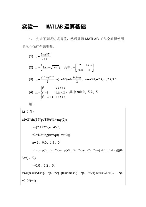
实验一 MATLAB 运算基础1、 先求下列表达式得值,然后显示MATLAB 工作空间得使用情况并保存全部变量。
(1) 0122sin 851z e =+(2) 21ln(2z x =+,其中2120.455i x +⎡⎤=⎢⎥-⎣⎦ (3) 0.30.330.3sin(0.3)ln , 3.0, 2.9,,2.9,3.022a a e e a z a a --+=++=--L (4) 2242011122123t t z t t t t t ⎧≤<⎪=-≤<⎨⎪-+≤<⎩,其中t =0:0、5:2、5 解:4、 完成下列操作:(1) 求[100,999]之间能被21整除得数得个数。
(2) 建立一个字符串向量,删除其中得大写字母。
解:(1) 结果:(2)、 建立一个字符串向量 例如:ch='ABC123d4e56Fg9';则要求结果就是:实验二 MATLAB 矩阵分析与处理1、 设有分块矩阵33322322E R A O S ⨯⨯⨯⨯⎡⎤=⎢⎥⎣⎦,其中E 、R 、O 、S 分别为单位矩阵、随机矩阵、零矩阵与对角阵,试通过数值计算验证22E R RS A OS +⎡⎤=⎢⎥⎣⎦。
解: M 文件如下;5、 下面就是一个线性方程组:1231112340.951110.673450.52111456x x x ⎡⎤⎢⎥⎡⎤⎡⎤⎢⎥⎢⎥⎢⎥⎢⎥=⎢⎥⎢⎥⎢⎥⎢⎥⎢⎥⎢⎥⎣⎦⎣⎦⎢⎥⎢⎥⎣⎦(1) 求方程得解。
(2) 将方程右边向量元素b 3改为0、53再求解,并比较b 3得变化与解得相对变化。
(3) 计算系数矩阵A 得条件数并分析结论。
解: M 文件如下:实验三 选择结构程序设计1、 求分段函数得值。
2226035605231x x x x y x x x x x x x ⎧+-<≠-⎪=-+≤<≠≠⎨⎪--⎩且且及其他用if 语句实现,分别输出x=-5、0,-3、0,1、0,2、0,2、5,3、0,5、0时得y 值。
MATLAB实验二运算基础答案

实验二、MA TLAB运算基础一、实验目的掌握MA TLAB各种表达式的书写规则及常用函数的使用。
掌握MA TLAB中字符串、元胞数组和结构的常用函数的使用。
二、实验内容及步骤1、设有矩阵A和B,A=[1 2 3 4 5;6 7 8 9 10;11 12 13 14 15;16 1718 19 20;21 22 23 24 25],B=[3 0 16;17 -6 9;0 23 -4;9 7 0;4 1311]1)求它们的乘积C2)将矩阵C的右下角3x2子矩阵赋给D>> A=[1:1:5;6:1:10;11:1:15;16:1:20;21:1:25];B=[3 0 16;17 -6 9;0 23 -4;9 7 0;4 13 11];...C=A*B,D=C(3:5,2:3)C =93 150 77258 335 237423 520 397588 705 557753 890 717D =520 397705 557890 7172、完成下列操作1)求[100,999]之间能被61整除的数及其个数(提示:先利用冒号表达式,再利用find和length函数。
)>> A=[100:999];B=find(rem(A,61)==0),B_total=length(B)B =23 84 145 206 267 328 389 450 511 572633 694 755 816 877B_total =152)建立一个字符串向量,删除其中的大写字母(提示:利用find函数和空矩阵。
)>> a=['MA TLAB is important'], b=abs(a); c=find(b<=90 & b>=65) , a(c)=[],a =MA TLAB is importantc = 1 2 3 4 5 6a =is important⑶已知A=[23 10 -78 0;41 -45 65 5;32 5 0 32;6 -5492 14],取出其前3行构成矩阵B,其前两列构成矩阵C,其左下角3x2子矩阵构成矩阵D,B与C的乘积构成矩阵E,分别求E<D、E&D、E|D、~E|~D。
MATLAB实验二

3. 三维图形
• 三、视点
➢view(az,el)-------------设置观察点方向
az为方位角,el为仰角。 • 方位角为视点位置在XY平面上的投影与X轴形成的角度,
正值表示逆时针,负值表示顺时针。 • 仰角为XY平面的上仰或下俯角,正值表示视点在XY平
面上方,负值表示视点在XY平面下方。
figure grid gtext hold subplot text title xlabel ylabel
创建图形窗口 放置坐标网格线 用鼠标放置文本 保持当前图形窗口内容 创建子图 放置文本 放置图形标题 放置X轴坐标标记 放置Y轴坐标标记
3. 三维图形 • 一、 plot3函数
• 将二维函数plot的功能扩展到三维空间,绘制三维图形。 • 函数格式:plot3(x1,y1,z1,c1,x2,y2,z2,c2,…)
theta=[0:0.01:2*pi];
rho=sin(2*theta).*cos(2*theta);
polar(theta,rho); 绘制极坐标图命令
title('polar plot');
例9、程序:
theta=linspace(0, 2*pi);
r=cos(4*theta);
polar(theta, r);
所组成的画面。
4. 动画设计
• 【例14】 播放一个不断变化的眼球程序段。
• m=moviein(20); 建立一个20个列向量组成的矩阵
• for j=1:20
•
plot(fft(eye(j+10))) %绘制出每一幅眼球图并保存到m矩阵中
• m(:,j)=getframe;
matlab第二章实训报告

佛山科学技术学院《MATLAB教程第二章实训》报告专业姓名成绩班级学号日期一、目的1.学习matlab的数据类型2.矩阵和数组的算术运算3.字符串4.时间和日期5.结构体和元胞数组6.多维数组7.逻辑运算和关系运算8.数组的信息获取9.多项式二、步骤1.学习matlab的数据类型Matlab R2010a定义了15种基本的数据类型,包括整型、浮点型、字符型和逻辑型等。
用户甚至可以定义自己的数据类型。
Matlab内部的任何数据类型,都是按照数组的形式进行储存和运算的。
数值型包括整数和浮点数,其中整数包括有符号数和无符号数,浮点数包括单精度型和双精度型。
在默认情况下,matlab默认将所有数值都按照双精度浮点数类型来存储和操作。
(1)常数和变量Matlab的常数采用十进制表示,可以用带小数点的形式直接表示,也可以用科学记数法。
数值的表示范围是10^-309-10^309。
变量是数值计算的基本单元。
Matlab与其他的高级语言不同,变量使用是无需先定义,其名称就是第一次合法出现时的名称,因此用起来很便捷。
Matlab的变量命名有一定的规则:a.变量区分字母的大小写。
例如,“a”和“A”是不同的变量。
b.变量名不能超过63个字符,第63个字符后的字符会被忽略。
c.变量名必须以字母开头,变量名的组成可以是任意字母、数字或者下划线,但不能有空格和标点符号。
d.关键字(如if\while等)不能作为变量名。
在matlab中的所有表示符号包括函数名、文件名都是遵循变量名的命名规则。
Matlab中有一些自己的特殊变量,是由系统预先自动定义的,例如:ans——运算结果的默认变量名Pi——圆周率πEps——浮点数的相对误差Inf或inf——无穷大Nan或nan——不定值i或j——i=j=-1^1/2,虚数单位Nargin——函数的输入变量数目Nargout——函数的输出变量数目Realmin——最小的可用正实数Realmax——最大的可用正实数(2)整数和浮点数Matlab提供了8种内置的整数类型,为了在使用时提高运行速度和存储空间,应该尽量使用字节少的数据类型,可以使用类型转换函数将各种整数类型强制相互转换。
MATLAB实验
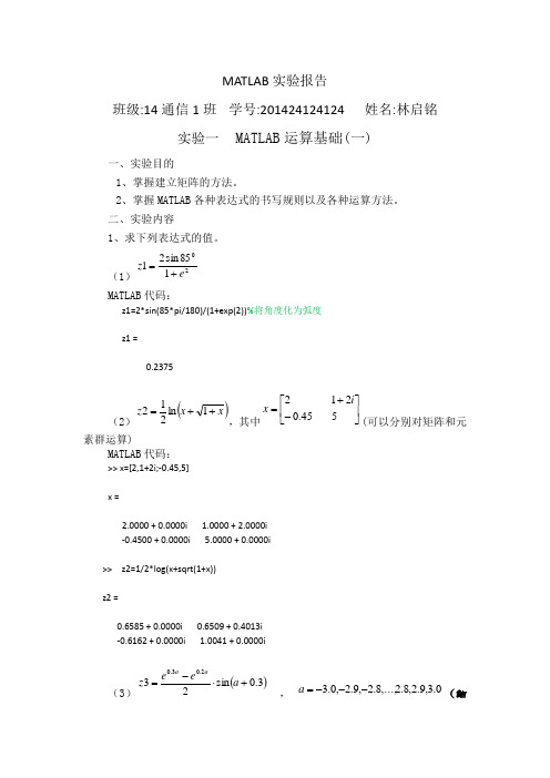
MATLAB 实验报告班级:14通信1班 学号:201424124124 姓名:林启铭实验一 MATLAB 运算基础(一)一、实验目的1、掌握建立矩阵的方法。
2、掌握MATLAB 各种表达式的书写规则以及各种运算方法。
二、实验内容1、求下列表达式的值。
(1)20185sin 21ez += MATLAB 代码:z1=2*sin(85*pi/180)/(1+exp(2))%将角度化为弧度z1 =0.2375(2)()x x z ++=1ln 212,其中⎢⎣⎡-=45.02x ⎥⎦⎤+521i (可以分别对矩阵和元素群运算)MATLAB 代码:>> x=[2,1+2i;-0.45,5]x =2.0000 + 0.0000i 1.0000 + 2.0000i-0.4500 + 0.0000i 5.0000 + 0.0000i>> z2=1/2*log(x+sqrt(1+x))z2 =0.6585 + 0.0000i 0.6509 + 0.4013i-0.6162 + 0.0000i 1.0041 + 0.0000i(3)()3.0sin 232.03.0+⋅-=a e e z aa , 0.3,9.2,8.2,...,8.2,9.2,0.3---=a (结果请用图形表示)(提示:利用冒号表达式生成a 向量;求各点的函数值时用点乘运算)MATLAB 代码:>> a=-3.0:0.1:3.0;%利用冒号表达式生成a 向量,加分号结尾避免大量数据刷屏 >> z3=(exp(0.3.*a)-exp(0.2.*a)).*sin(a+0.3)/2;>> plot(a,z3);%绘制出以a 为自变量,z3为因变量的曲线>>曲线图:2、已知⎢⎢⎢⎣⎡=33412A 65734⎥⎥⎥⎦⎤-7874 和 ⎢⎢⎢⎣⎡=321B 203-⎥⎥⎥⎦⎤-731 求下列表达式的值:(1)A+6*B 和A-B+I (其中I 为单位矩阵)。
- 1、下载文档前请自行甄别文档内容的完整性,平台不提供额外的编辑、内容补充、找答案等附加服务。
- 2、"仅部分预览"的文档,不可在线预览部分如存在完整性等问题,可反馈申请退款(可完整预览的文档不适用该条件!)。
- 3、如文档侵犯您的权益,请联系客服反馈,我们会尽快为您处理(人工客服工作时间:9:00-18:30)。
Experiment 1. Fundamental Knowledge of Matlab (II) 【Experimental Purposes】1、熟悉并掌握MATLAB的工作环境。
2、运行简单命令,实现数组及矩阵的输入输出,了解在MATLAB下如何绘图。
【Experimental Principle】1. VectorsLet's start off by creating something simple, like a vector. Enter each element of the vector (separated by a space) between brackets, and set it equal to a variable. For example, to create the vector a, enter into the MATLAB command window (you can "copy" and "paste" from your browser into MATLAB to make it easy):a = [1 2 3 4 5 6 9 8 7]MATLAB should return:a =1 2 3 4 5 6 9 8 7To generate a series that does not use the default of incrementing by 1, specify an additional value with the colon operator (first:step:last). In between the starting and ending value is a step value that tells MATLAB how much to increment (or decrement, if step is negative) between each number it generates. To generate a vector with elements between 0 and 20, incrementing by 2(this method is frequently used to create a time vector), uset = 0:2:20t =0 2 4 6 8 10 12 14 16 18 20Manipulating vectors is almost as easy as creating them. First, suppose you would like to add 2 to each of the elements in vector 'a'. The equation for that looks like:b = a + 2b =3 4 5 6 7 8 11 10 9Now suppose, you would like to add two vectors together. If the two vectors are the same length, it is easy. Simply add the two as shown below:c = a + bc =4 6 8 10 12 14 20 18 16Subtraction of vectors of the same length works exactly the same way.MATLAB sometimes stores such a list in a matrix with just one row, and other times in a matrix with just one column. In the first instance, such a 1-row matrix is called a row-vector; in thesecond instance, such a 1-column matrix is called a column-vector. Either way, these are merely different ways for storing vectors, not different kinds of vectors.2. Matrices and ArraysThe most basic MATLAB data structure is the matrix: a two-dimensional, rectangularly shaped data structure capable of storing multiple elements of data in an easily accessible format. These data elements can be numbers, characters, logical states of true or false, or even other MATLAB structure types. MATLAB uses these two-dimensional matrices to store single numbers and linear series of numbers as well. In these cases, the dimensions are 1-by-1 and 1-by-n respectively, where n is the length of the numeric series. MATLAB also supports data structures that have more than two dimensions. These data structures are referred to as arrays in the MATLAB documentation.MATLAB is a matrix-based computing environment. All of the data that you enter into MATLAB is stored in the form of a matrix or a multidimensional array. Even a single numeric value like 100 is stored as a matrix (in this case, a matrix having dimensions 1-by-1):A = 100;Name Size Bytes ClassA 1x1 8 double arrayEntering matrices into MATLAB is the same as entering a vector, except each row of elements is separated by a semicolon (;) or a return:B = [1 2 3 4;5 6 7 8;9 10 11 12]B =1 2 3 45 6 7 89 10 11 12B = [ 1 2 3 45 6 7 89 10 11 12]B =1 2 3 45 6 7 89 10 11 12The square brackets operator constructs two-dimensional matrices only, (including 0-by-0, 1-by-1, and 1-by-n matrices).Matrices in MATLAB can be manipulated in many ways. For one, you can find the transpose of a matrix using the apostrophe key:C = B'C =1 5 92 6 103 7 114 8 12It should be noted that if C had been complex, the apostrophe would have actually given the complex conjugate transpose. To get the transpose, use .' (the two commands are the same if the matix is not complex).Now you can multiply the two matrices B and C together. Remember that order matters when multiplying matrices.D = B * CD =30 70 11070 174 278110 278 446D= C * BD =107 122 137 152122 140 158 176137 158 179 200152 176 200 224Another option for matrix manipulation is that you can multiply the corresponding elements of two matrices using the .* operator (the matrices must be the same size to do this).E = [1 2;3 4]F = [2 3;4 5]G = E .* FE =1 23 4F =2 34 5G =2 612 20If you have a square matrix, like E, you can also multiply it by itself as many times as you like by raising it to a given power.E^3ans =37 5481 118If wanted to cube each element in the matrix, just use the element-by-element cubing.E.^3ans =1 827 64You can also find the inverse of a matrix:X = inv(E)X =-2.0000 1.00001.5000 -0.5000or its eigenvalues:eig(E)ans =-0.37235.3723There is even a function to find the coefficients of the characteristic polynomial of a matrix. The "poly" function creates a vector that includes the coefficients of the characteristic polynomial.p = poly(E)p =1.0000 -5.0000 -2.0000Remember that the eigenvalues of a matrix are the same as the roots of its characteristic polynomial:roots(p)ans =5.3723-0.37233. FunctionsTo make life easier, MATLAB includes many standard functions. Each function is a block of code that accomplishes a specific task. MATLAB contains all of the standard functions such as sin, cos, log, exp, sqrt, as well as many others. Commonly used constants such as pi, and i or j for the square root of -1, are also incorporated into MATLAB.sin(pi/4)ans =0.7071To determine the usage of any function, type help [function name] at the MATLAB command window. MATLAB even allows you to write your own functions with the function command; follow the link to learn how to write your own functions and see a listing of the functions we created for this tutorial.4. PlottingIt is also easy to create plots in MATLAB. Suppose you wanted to plot a sine wave as a function of time. First make a time vector (the semicolon after each statement tells MATLAB we don't want to see all the values) and then compute the sin value at each time.t=0:0.25:7;y = sin(t);plot(t,y)The plot contains approximately one period of a sine wave. Basicplotting is very easy in MATLAB, and the plot command hasextensive add-on capabilities. I would recommend you visit theplotting page to learn more about it.5. PolynomialsIn MATLAB, a polynomial is represented by a vector. To create a polynomial in MATLAB, simply enter each coefficient of the polynomial into the vector in descending order. For instance, let's say you have the following polynomial:43231529s s s s +--+ To enter this into MATLAB, just enter it as a vector in the following mannerx = [1 3 -15 -2 9]x =1 3 -15 -2 9MATLAB can interpret a vector of length n+1 as an nth order polynomial. Thus, if yourpolynomial is missing any coefficients, you must enter zeros in the appropriate place in the vector. For example,41s + would be represented in MA TLAB as:y = [1 0 0 0 1]You can find the value of a polynomial using the polyval function. For example, to find the value of the above polynomial at s=2,z = polyval([1 0 0 0 1],2)z =17You can also extract the roots of a polynomial. This is useful when you have a high-order polynomial such as43231529s s s s +--+ Finding the roots would be as easy as entering the following command;roots([1 3 -15 -2 9])ans =-5.57452.5836-0.79510.7860Let's say you want to multiply two polynomials together. The product of two polynomials is found by taking the convolution of their coefficients. MATLAB's function conv that will do this for you.x = [1 2];y = [1 4 8];z = conv(x,y)z =1 6 16 16Dividing two polynomials is just as easy. The deconv function will return the remainder as well as the result. Let's divide z by y and see if we get x.[xx, R] = deconv(z,y)xx =1 2R =0 0 0 0As you can see, this is just the polynomial/vector x from before. If y had not gone into z evenly, the remainder vector would have been something other than zero.If you want to add two polynomials together which have the same order, a simple z=x+y will work (the vectors x and y must have the same length). In the general case, the user-defined function, polyadd can be used. To use polyadd, copy the function into an m-file, and then use it just as you would any other function in the MATLAB toolbox. Assuming you had the polyadd function stored as a m-file, and you wanted to add the two uneven polynomials, x and y, you could accomplish this by entering the command:z = polyadd(x,y)x =1 2y =1 4 8z =1 5 10【Experiment contents and procedure】1、运行简单命令,实现数组及矩阵的输入输出;2、运行特殊矩阵的输入及输出;MATLAB has a number of functions that create different kinds of matrices. Some create specialized matrices like the Hankel or Vandermonde matrix. The functions shown in the table below create matrices for more general use.However, you can easily build basic arrays of any numeric type using the ones, zeros, and eye functions.A = magic(5)A =17 24 1 8 1523 5 7 14 164 6 13 20 2210 12 19 21 311 18 25 2 9Note that the elements of each row, each column, and each main diagonal add up to the same value: 65.3、进行简单的MATLAB绘图;4、多项式的输入及输出。