LCIS A Boundary Hierarchy For Detail-Preserving Contrast LCIS为保细节层次对比边界

合集下载

(完整word版)ICC(A)条款英文版

1/1/82INSTITUTE CARGO CLAUSES （A)RISKS COVERED1.This insurance covers all risks of loss of or damage to the subject-matter insured except asprovided in Clauses 4, 5， 6 and 7 below。

2.This insurance covers general average and salvage charges, adjusted or determined according tothe contract of affreightment and/or the governing law and practice， incurred to avoid or in connection with the avoidance of loss from any cause except those excluded in Clauses 4, 5， 6 and 7 or elsewhere in this insurance。

3.This insurance is extended to indemnify the Assured against such proportion of liability underthe contract of affreightment "Both to Blame Collision” Clause as is in respect of a loss recoverable hereunder。

In the event of any claim by shipowners under the said Clause the Assured agree to notify the Underwriters who shall have the right， at their own cost and expense, to defend the Assured against such claim。

COMSOL案例详解液滴models.mfl.droplet_breakup(优选.)

Droplet Breakup in a T-Junction IntroductionEmulsions consist of small liquid droplets immersed in another liquid, typically oil in water or water in oil. Emulsions find wide application in the production of food, cosmetics, and pharmaceutical products. The properties and quality of an emulsion typically depend on the size and the distribution of the droplets. This example studies in detail how to create uniform droplets in a microchannel T-junction.Setting up the model you can make use of the Laminar Two-Phase Flow, Level Set interface. The model uses the predefined wetted wall boundary condition at the solid walls, with a contact angle of 135°. From the results, you can determine the size of the created droplets and the rate with which they are produced.Model DefinitionFigure 1 shows the geometry of the T-shaped microchannel with a rectangular cross section. For the separated fluid elements to correspond to droplets, the geometry is modeled in 3D. Due to symmetry, it is sufficient to model only half of the junction geometry. The modeling domain is shown in Figure 1. The fluid to be dispersed intosmall droplets, Fluid 2, enters through the vertical channel. The other fluid, Fluid 1, flows from the right to left through the horizontal channel.Inlet, fluid 2Inlet, fluid 1Initial fluid interface OutletFigure 1: The modeling domain of the T-junction.The problem described is straight forward to set up with the Laminar Two-Phase Flow, Level Set interface. The interface sets up a momentum transport equation, a continuity equation, and a level set equation for the level set variable. The fluid interface is defined by the 0.5 contour of the level set function.The interface uses the following equations:In the equations above, ρ denotes density (kg/m 3), u velocity (m/s), t time (s), μ dynamic viscosity (Pa·s), p pressure (Pa), and F st the surface tension force (N/m 3). Furthermore, φ is the level set function, and γ and ε are numerical stabilization parameters. The density and viscosity are calculated fromρt∂∂u ρu ∇⋅()u +∇p –I μ∇u ∇u ()T +()+[]F st +⋅=∇u ⋅0=∂φ∂t -----u ∇φ⋅+γ∇φ–1φ–()∇φ∇φ----------ε∇φ+⎝⎭⎛⎫⋅=where ρ1, ρ2, μ1, and μ2 are the densities and viscosities of Fluid 1 and Fluid 2.P H Y S I C A L P A R A M E T E R SThe two liquids have the following physical properties:QUANTITY VALUE, FLUID 1VALUE, FLUID 2Density (kg/m 3)10001000Dynamic viscosity (Pa·s)0.001950.00671The surface tension coefficient is 5·10−3 N/m.B O U N D A R YC O ND I T I O N SAt both inlets, Laminar inflow conditions with prescribed volume flows are used. At the outflow boundary, the Pressure, no viscous stress condition is set. The Wetted wall boundary condition applies to all solid boundaries with the contact angle specified as 135° and a slip length equal to the mesh size parameter, h . The contact angle is the angle between the fluid interface and the solid wall at points where the fluid interface attaches to the wall. The slip length is the distance to the position outside the wall where the extrapolated tangential velocity component is zero (see Figure 2).Fluid 1Fluid 2Wall θWallβu Figure 2: The contact angle, θ, and the slip length, β.ρρ1ρ2ρ1–()φ+=μμ1μ2μ1–()φ+=Results and DiscussionFigure 3 shows the fluid interface (the level set function φ0.5=) and velocitystreamlines at various times. The first droplet is formed after approximately0.03 s.Figure 3: Velocity streamlines, velocity on the symmetry plane, and the phase boundary at t = 0.02 s, 0.04 s, 0.06 s, and 0.08 s.You can calculate the effective diameter, d eff —that is, the diameter of a sphericaldroplet with the same volume as the formed droplet—using the following expression:(1)Here, Ω represents the leftmost part of the horizontal channel, where x < −0.2 mm. In this case, the results show that d eff is about 0.12 mm. The results are in fair agreement with those presented in Ref. 1.d eff 234π------φ0.5>()Ωd Ω 3⋅=Reference1. S. van der Graaf, T. Nisisako, C. G. P. H. Schroën, R. G. M. van der Sman, and R. M. Boom, “Lattice Boltzmann Simulations of Droplet Formation in a T-Shaped Microchannel,” Langmuir, vol. 22, pp. 4144–4152, 2006.Application Library path: Microfluidics_Module/Two-Phase_Flow/droplet_breakupModeling InstructionsFrom the File menu, choose New.N E W1In the New window, click Model Wizard.M O D E L W I Z A R D1In the Model Wizard window, click 3D.2In the Select physics tree, select Fluid Flow>Multiphase Flow>Two-Phase Flow, Level Set>Laminar Two-Phase Flow, Level Set (tpf).3Click Add.4Click Study.5In the Select study tree, select Preset Studies>Transient with Phase Initialization.6Click Done.G E O M E T R Y11In the Model Builder window, under Component 1 (comp1) click Geometry 1.2In the Settings window for Geometry, locate the Units section.3From the Length unit list, choose mm.Work Plane 1 (wp1)1On the Geometry toolbar, click Work Plane.2In the Settings window for Work Plane, locate the Plane Definition section.3From the Plane list, choose xz-plane.Rectangle 1 (r1)1On the Geometry toolbar, click Primitives and choose Rectangle.2In the Settings window for Rectangle, locate the Size section.3In the Width text field, type 0.1.4In the Height text field, type 0.4.5Locate the Position section. In the yw text field, type 0.1.Rectangle 2 (r2)1On the Geometry toolbar, click Primitives and choose Rectangle.2In the Settings window for Rectangle, locate the Size section.3In the Width text field, type 1.4In the Height text field, type 0.1.5Locate the Position section. In the xw text field, type -0.7.Plane Geometry1On the Geometry toolbar, click Build All.2Click the Zoom Extents button on the Graphics toolbar.Polygon 1 (pol1)1On the Geometry toolbar, click Primitives and choose Polygon.2In the Settings window for Polygon, locate the Object Type section.3From the Type list, choose Open curve.4Locate the Coordinates section. In the xw text field, type 0 0.1.5In the yw text field, type 0.2 0.2.Plane GeometryRight-click Component 1 (comp1)>Geometry 1>Work Plane 1 (wp1)>Plane Geometry>Polygon 1 (pol1) and choose Build Selected.Polygon 2 (pol2)1On the Geometry toolbar, click Primitives and choose Polygon.2In the Settings window for Polygon, locate the Coordinates section.3In the xw text field, type 0.1 0.1.4In the yw text field, type 0 0.1.Work Plane 1 (wp1)Right-click Component 1 (comp1)>Geometry 1>Work Plane 1 (wp1)>PlaneGeometry>Polygon 2 (pol2) and choose Build Selected .Extrude 1 (ext1)1On the Geometry toolbar, click Extrude .2In the Settings window for Extrude, locate the Distances from Plane section.3In the table, enter the following settings:4Right-click Component 1 (comp1)>Geometry 1>Extrude 1 (ext1) and choose Build Selected .5Click the Zoom Extents button on the Graphics toolbar.Form Union (fin)1In the Model Builder window, under Component 1 (comp1)>Geometry 1 right-click Form Union (fin) and choose Build Selected . The geometry should look like in Figure 1.M A T E R I A L SMaterial 1 (mat1)1In the Model Builder window, under Component 1 (comp1) right-click Materials and choose Blank Material .2Right-click Material 1 (mat1) and choose Rename .3In the Rename Material dialog box, type Fluid 1 in the New label text field.4Click OK .5In the Settings window for Material, locate the Material Contents section.6In the table, enter the following settings:Distances (mm)0.05Property Name ValueUnit Property group Density rho 1e3[kg/m^3]kg/m³Basic Dynamic viscosity mu 1.95e-3[Pa*s]Pa·s BasicMaterial 2 (mat2)1In the Model Builder window, right-click Materials and choose Blank Material .2Right-click Material 2 (mat2) and choose Rename .3In the Rename Material dialog box, type Fluid 2 in the New label text field.4Click OK .5In the Settings window for Material, click to expand the Material properties section.6Locate the Material Properties section. In the Material properties tree, select Basic Properties>Density .7Click Add to Material .8In the Material properties tree, select Basic Properties>Dynamic Viscosity .9Click Add to Material .10Locate the Material Contents section. In the table, enter the following settings:D E F I N I T I O N SStep 1 (step1)1On the Home toolbar, click Functions and choose Local>Step .2In the Settings window for Step, locate the Parameters section.3In the Location text field, type 1e-3.4Click to expand the Smoothing section. In the Size of transition zone text field, type 2e-3.Add an integration operator that you will use to calculate the effective droplet diameter according to Equation 1 in the Model Definition section.Integration 1 (intop1)1On the Definitions toolbar, click Component Couplings and choose Integration .2In the Settings window for Integration, locate the Source Selection section.3From the Selection list, choose All domains .Property Name ValueUnit Property group Density rho 1e3[kg/m^3]kg/m³Basic Dynamic viscosity mu 6.71e-3[Pa*s]Pa·s BasicVariables 11On the Definitions toolbar, click Local Variables .2In the Settings window for Variables, locate the Variables section.3In the table, enter the following settings:L A M I N A R T W O -P H A S E F L O W, L E V E L S E T (T P F )The mesh can be controlled very well in this model, which makes it possible to use a lower element order without reducing the accuracy.1In the Model Builder window’s toolbar, click the Show button and select Discretization in the menu.2In the Model Builder window, expand the Component 1 (comp1)>Laminar Two-Phase Flow, Level Set (tpf) node, then click Laminar Two-Phase Flow, Level Set (tpf).3In the Settings window for Laminar Two-Phase Flow, Level Set, click to expand the Discretization section.4From the Discretization of fluids list, choose P1 + P1.Fluid Properties 11In the Model Builder window, under Component 1 (comp1)>Laminar Two-Phase Flow, Level Set (tpf) click Fluid Properties 1.2In the Settings window for Fluid Properties, locate the Fluid 1 Properties section.3From the Fluid 1 list, choose Fluid 1 (mat1).4Locate the Fluid 2 Properties section. From the Fluid 2 list, choose Fluid 2 (mat2).5Locate the Surface Tension section. From the Surface tension coefficient list, choose User defined . In the σ text field, type 5e-3[N/m].6Locate the Level Set Parameters section. In the γ text field, type 0.05[m/s].7In the εls text field, type 5e-6[m].NameExpression Unit Description V10.4e-6/3600*step1(t[1/s])[m^3/s]m³/s Volume flow, inlet 1V20.2e-6/3600*step1(t[1/s])[m^3/s]m³/s Volume flow, inlet 2d_eff 2*(intop1((phils>0.5)*(x<-0.2[mm]))*3/(4*pi))^(1/3)m Effective droplet diameterWall 1Because this is the default boundary condition node, you cannot modify the selection explicitly. Instead, you override the default condition where it is not applicable by adding other boundary conditions.1In the Model Builder window, under Component 1 (comp1)>Laminar Two-Phase Flow, Level Set (tpf) click Wall 1.2In the Settings window for Wall, locate the Boundary Condition section.3From the Boundary condition list, choose Wetted wall.4In the θw text field, type 3*pi/4[rad].5In the β text field, type 5e-6[m].Initial Interface 11In the Model Builder window, under Component 1 (comp1)>Laminar Two-Phase Flow, Level Set (tpf) click Initial Interface 1.2Select Boundary 11 only.Initial Values 21On the Physics toolbar, click Domains and choose Initial Values.2Select Domain 3 only.3In the Settings window for Initial Values, locate the Initial Values section.4From the Fluid initially in domain list, choose Fluid 2.For Domains 1 and 2, the default initial value settings apply.Inlet 11On the Physics toolbar, click Boundaries and choose Inlet.2Select Boundary 22 only.3In the Settings window for Inlet, locate the Boundary Condition section.4From the list, choose Laminar inflow.5Locate the Laminar Inflow section. Click the Flow rate button.6In the V0 text field, type V1.7In the L entr text field, type 0.01[m].Inlet 21On the Physics toolbar, click Boundaries and choose Inlet.2Select Boundary 12 only.3In the Settings window for Inlet, locate the Level Set Condition section.4In the V f text field, type 1.5Locate the Boundary Condition section. From the list, choose Laminar inflow.6Locate the Laminar Inflow section. Click the Flow rate button.7In the V0 text field, type V2.8In the L entr text field, type 0.01[m].Outlet 11On the Physics toolbar, click Boundaries and choose Outlet.2Select Boundary 1 only.Symmetry 11On the Physics toolbar, click Boundaries and choose Symmetry.2Select Boundaries 5, 13, 14, and 21 only.M E S H1Mapped 11In the Model Builder window, under Component 1 (comp1) right-click Mesh 1 andchoose More Operations>Mapped.2Select Boundaries 2, 7, 10, and 16 only.Distribution 11Right-click Component 1 (comp1)>Mesh 1>Mapped 1 and choose Distribution.2Select Edge 3 only.3In the Settings window for Distribution, locate the Distribution section.4In the Number of elements text field, type 160.Distribution 21Right-click Mapped 1 and choose Distribution.2Select Edges 1 and 9 only.3In the Settings window for Distribution, locate the Distribution section.4In the Number of elements text field, type 20.Distribution 31Right-click Mapped 1 and choose Distribution.2Select Edges 12 and 28 only.3In the Settings window for Distribution, locate the Distribution section.11|D R O P L E T B R E A K U P I N A T-J U N C T I O N4From the Distribution properties list, choose Predefined distribution type.5In the Number of elements text field, type 25.6In the Element ratio text field, type 4.Distribution 41Right-click Mapped 1 and choose Distribution.2Select Edges 24 and 27 only.3In the Settings window for Distribution, locate the Distribution section.4From the Distribution properties list, choose Predefined distribution type.5In the Number of elements text field, type 20.6In the Element ratio text field, type 3.7Select the Reverse direction check box.Mapped 1Right-click Mapped 1 and choose Build Selected.Swept 11Right-click Mesh 1 and choose Swept.2In the Settings window for Swept, click to expand the Source faces section.3Locate the Source Faces section. Select the Active toggle button.4Select Boundaries 2, 7, and 10 only.Distribution 11Right-click Component 1 (comp1)>Mesh 1>Swept 1 and choose Distribution.2In the Settings window for Distribution, locate the Distribution section.3In the Number of elements text field, type 10.12|D R O P L E T B R E A K U P I N A T-J U N C T I O N4Click the Build All button.S T U D Y1Step 2: Time Dependent1In the Model Builder window, expand the Study 1 node, then click Step 2: Time Dependent.2In the Settings window for Time Dependent, locate the Study Settings section.3In the Times text field, type range(0,5e-3,0.08).4Click to expand the Results while solving section. Locate the Results While Solvingsection. Select the Plot check box.5From the Plot group list, choose Default.This choice means that the Graphics window will show a surface plot of the volumefraction of Fluid 1 while solving, and this plot will be updated at each 5 ms output timestep.Manually tune the solver sequence for optimal performance and accuracy.Solution 11On the Study toolbar, click Show Default Solver.2In the Model Builder window, expand the Solution 1 node, then click Time-Dependent Solver 1.13|D R O P L E T B R E A K U P I N A T-J U N C T I O N3In the Settings window for Time-Dependent Solver, click to expand the Time stepping section.4Locate the Time Stepping section. From the Method list, choose Generalized alpha.5Select the Time step increase delay check box.6In the associated text field, type 3.7In the Amplification for high frequency text field, type 0.3.8From the Predictor list, choose Constant.9In the Model Builder window, expand the Study 1>Solver Configurations>Solution1>Time-Dependent Solver 1 node.10Right-click Study 1>Solver Configurations>Solution 1>Time-Dependent Solver 1 andchoose Iterative.11In the Settings window for Iterative, locate the Error section.12In the Factor in error estimate text field, type 20.13In the Maximum number of iterations text field, type 200.14Right-click Study 1>Solver Configurations>Solution 1>Time-Dependent Solver1>Iterative 1 and choose Multigrid.15In the Model Builder window, expand the Study 1>Solver Configurations>Solution1>Time-Dependent Solver 1>Iterative 1>Multigrid 1 node.16Right-click Presmoother and choose SCGS.17In the Settings window for SCGS, locate the Main section.18Select the Vanka check box.19Under Variables, click Add.20In the Add dialog box, In the Variables list, choose comp1.tpf.Pinlinl1 andcomp1.tpf.Pinlinl2.21Click OK.22In the Model Builder window, expand the Study 1>Solver Configurations>Solution1>Time-Dependent Solver 1>Iterative 1>Multigrid 1>Postsmoother node.23Right-click Study 1>Solver Configurations>Solution 1>Time-Dependent Solver1>Iterative 1>Multigrid 1>Postsmoother and choose SCGS.24In the Settings window for SCGS, locate the Main section.25Select the Vanka check box.26Under Variables, click Add.14|D R O P L E T B R E A K U P I N A T-J U N C T I O N27In the Add dialog box, In the Variables list, choose comp1.tpf.Pinlinl1 and comp1.tpf.Pinlinl2.28Click OK.29In the Model Builder window, expand the Study 1>Solver Configurations>Solution1>Time-Dependent Solver 1>Iterative 1>Multigrid 1>Coarse Solver node, then clickDirect.30In the Settings window for Direct, locate the General section.31From the Solver list, choose PARDISO.32In the Model Builder window, collapse the Study 1>Solver Configurations>Solution1>Time-Dependent Solver 1 node.S T U D Y1Solution 11In the Model Builder window, collapse the Study 1>Solver Configurations>Solution1>Time-Dependent Solver 1 node.2In the Model Builder window, collapse the Solution 1 node.3On the Study toolbar, click Compute.4Click the Zoom Extents button on the Graphics toolbar.R E S U L T SThe first default plot group shows the volume fraction of fluid 1 as slice plot, and thesecond plot group shows a slice plot of the velocity combined with a contour plot ofthe volume fraction of fluid 1. Follow these steps to reproduce the series of velocityfield plots shown in Figure 3.3D Plot Group 31On the Home toolbar, click Add Plot Group and choose 3D Plot Group.2In the Model Builder window, under Results right-click 3D Plot Group 3 and choose Slice.3In the Settings window for Slice, click Replace Expression in the upper-right cornerof the Expression section. From the menu, choose Component 1>Laminar Two-PhaseFlow, Level Set>tpf.U - Velocity magnitude.4Locate the Plane Data section. From the Plane list, choose zx-planes.5From the Entry method list, choose Coordinates.6On the 3D Plot Group 3 toolbar, click Plot.15|D R O P L E T B R E A K U P I N A T-J U N C T I O N7In the Model Builder window, right-click 3D Plot Group 3 and choose Isosurface.8In the Settings window for Isosurface, locate the Levels section.9From the Entry method list, choose Levels.10In the Levels text field, type 0.5.11Locate the Coloring and Style section. From the Coloring list, choose Uniform.12From the Color list, choose Green.13Right-click 3D Plot Group 3 and choose Streamline.14In the Settings window for Streamline, locate the Streamline Positioning section.15From the Positioning list, choose Uniform density.16In the Separating distance text field, type 0.05.17Locate the Coloring and Style section. From the Line type list, choose Tube.18Select the Radius scale factor check box.19In the associated text field, type 2e-3.20From the Color list, choose Yellow.21In the Model Builder window, click 3D Plot Group 3.22In the Settings window for 3D Plot Group, locate the Data section.23From the Time (s) list, choose 0.02.24On the 3D Plot Group 3 toolbar, click Plot.25Click the Go to Default 3D View button on the Graphics toolbar.Compare the resulting plot with the upper-left plot in Figure 3.To reproduce the remaining three plots, plot the solution for the time values 0.04,0.06, and 0.08 s.Next, evaluate the effective droplet diameter computed according to Equation 1.Derived Values1On the Results toolbar, click Global Evaluation.2In the Settings window for Global Evaluation, click Replace Expression in theupper-right corner of the Expression section. From the menu, choose Component1>Definitions>Variables>d_eff - Effective droplet diameter.3Click the Evaluate button.16|D R O P L E T B R E A K U P I N A T-J U N C T I O NT A B L E1Go to the Table window.The result, roughly 0.12 mm, is displayed in the table in the Table window.Finally, generate a movie of the moving fluid interface and the velocity streamlines.R E S U L T SExport1In the Model Builder window, under Results right-click 3D Plot Group 3 and choose Player.COMSOL Multiphysics generates the movie and then plays it.To replay the movie, click the Play button on the Graphics toolbar.If you want to export a movie in GIF, Flash, or AVI format, right-click Export andcreate an Animation feature.17|D R O P L E T B R E A K U P I N A T-J U N C T I O N18|D R O P L E T B R E A K U P I N A T-J U N C T I O N。

ASTM材料与实验标准.E164

Designation:E164–03Standard Practice forUltrasonic Contact Examination of Weldments1This standard is issued under theﬁxed designation E164;the number immediately following the designation indicates the year of original adoption or,in the case of revision,the year of last revision.A number in parentheses indicates the year of last reapproval.A superscript epsilon(e)indicates an editorial change since the last revision or reapproval.This standard has been approved for use by agencies of the Department of Defense.1.Scope1.1This practice covers techniques for the ultrasonic A-scan examination of speciﬁc weld conﬁgurations joining wrought ferrous or aluminum alloy materials to detect weld disconti-nuities(Note1).The reﬂection method using pulsed waves is speciﬁed.Manual techniques are described employing contact of the search unit through a couplantﬁlm or water column.1.2This practice utilizes angle beams or straight beams,or both,depending upon the speciﬁc weld conﬁgurations.Prac-tices for special geometries such asﬁllet welds and spot welds are not included.The practice is intended to be used on thicknesses of0.250to8in.[6.4to203mm].N OTE1—This practice is based on experience with ferrous and alumi-num alloys.Other metallic materials can be examined using this practice provided reference standards can be developed that demonstrate that the particular material and weld can be successfully penetrated by an ultrasonic beam.N OTE2—For additional pertinent information see Practice E317, Terminology E1316,and Practice E587.1.3Values stated in inch-pound units are to be regarded as the standard.SI units are given for information only.1.4This standard does not purport to address all of the safety concerns,if any,associated with its use.It is the responsibility of the user of this standard to establish appro-priate safety and health practices and determine the applica-bility of regulatory limitations prior to use.2.Referenced Documents2.1ASTM Standards:E317Practice for Evaluating Performance Characteristics of Ultrasonic Pulse-Echo Examination Systems Without the Use of Electronic Measurement Instruments2E543Practice for Agencies Performing Nondestructive Testing2E587Practice for Ultrasonic Angle-Beam Examination by the Contact Method2E1316Terminology for Nondestructive Examinations2 2.2ASNT Standard:Practice SNT-TC-1A Personnel Qualiﬁcation and Certiﬁca-tion in Nondestructive Testing32.3ISO Standard:ISO2400Reference Block for the Calibration of Equipment for Ultrasonic Examination43.Signiﬁcance and Use3.1The techniques for ultrasonic examination of welds described in this practice are intended to provide a means of weld examination for both internal and surface discontinuities within the weld and the heat-affected zone.The practice is limited to the examination of speciﬁc weld geometries in wrought or forged material.3.2The techniques provide a practical method of weld examination for internal and surface discontinuities and are well suited to the task of in-process quality control.The practice is especially suited to the detection of discontinuities that present planar surfaces perpendicular to the sound beam. Other nondestructive tests may be used when porosity and slag inclusions must be critically evaluated.3.3When ultrasonic examination is used as a basis of acceptance of welds,there should be agreement between the manufacturer and the purchaser as to the speciﬁc reference standards and limits to be used.Examples of reference stan-dards are given in Section6.A detailed procedure for weld examination describing allowable discontinuity limits should be written and agreed upon.3.4Personnel Qualiﬁcation—In order to meet the intent of this recommended practice,it is essential that evaluation be performed by properly trained and qualiﬁed testing personnel. The user is referred to Practice SNT-TC-1A published by American Society of Nondestructive Testing(ASNT)or other equivalent programs.3.5Nondestructive Testing Agency Evaluation—Use of an NDT agency(as deﬁned in Practice E543)to perform the examination may be agreed upon by the using parties.If a1This practice is under the jurisdiction of ASTM Committee E07on Nonde-structive Testing and is the direct responsibility of Subcommittee E07.06onUltrasonic Method.Current edition approved August10,2003.Published October2003.Originally approved st previous edition approved in1997as E164-97.2Annual Book of ASTM Standards,V ol03.03.3Available from The American Society for Nondestructive Testing(ASNT),P.O. Box28518,1711Arlingate Ln.,Columbus,OH43228-0518.4Available from American National Standards Institute(ANSI),25W.43rd St., 4th Floor,New York,NY10036.Copyright©ASTM International,100Barr Harbor Drive,PO Box C700,West Conshohocken,PA19428-2959,United States.systematic assessment of the capability of the agency is speciﬁed,a documented procedure such as Practice E 543shall be used as the basis for evaluation.4.Search Units4.1Angle-Beam requirements for angle-beam search units are determined by the test variables.The examination proce-dure should be established by taking into consideration vari-ables such as weld thickness,available surface,maximum allowable ﬂaw size,ﬂaw orientation,and the acoustic proper-ties of the material.Consideration should also be given to the desirability of using comparable wave lengths within the materials where both a longitudinal-wave examination and an angle-beam shear-wave examination are employed.This can be accomplished by conducting the straight-beam (longitudinal-wave)examination at approximately two times the frequency of the angle-beam (shear-wave)examination.4.2Frequencies of 1.0to 5MHz are generally employed for angle-beam (shear-wave)and for straight-beam (longitudinal-wave)examination.4.3Transducer sizes recommended for weld examination range from a minimum of 1⁄4-in.[6.4-mm]diameter or 1⁄4-in.square to 1in.[25.4mm]square or 11⁄8-in.[28.6-mm]diameter.5.Standardization5.1Two methods of angle-beam standardization are in general use:the polar,and the rectangular,coordinate methods.5.1.1The polar coordinate method requires measurements of the beam centerline at the search unit/work interface and the beam angle in a test block,and the instrument sweep is calibrated along the beam line.Test information is graphically converted into position and depth coordinates for reﬂector location.The polar method is detailed in Annex A1.5.1.2The rectangular coordinate method requires measure-ment of the position of the reﬂector from the front of the search unit,and the instrument sweep is calibrated for depth to the reﬂector as it is moved to different positions in the beam providing a distance-amplitude curve.Test information is read directly for position and depth to the reﬂector.The rectangular coordinate method is detailed in Annex A2.6.Reference Standards6.1IIW-type reference blocks are a class of reference blocks for checking and calibrating ultrasonic instrumentation,which meet the basic geometrical conﬁguration described in ISO 2400but which may deviate in such aspects as non-metric dimensioning,alternate materials,additional reﬂectors,and differences of scale details.IIW-type blocks are primarily intended for characterizing and calibrating angle-beam sys-tems,but also provide features for such uses as straight-beam resolution and sensitivity checks.N OTE 3—Discussion of the differences among various versions of “IIW-Type”reference blocks,illustrations of typical conﬁgurations and an extensive bibliography can be found in a published reference.56.1.1Only blocks fully meeting all the requirements of ISO 2400should be referred to as IIW reference blocks.6.1.2Blocks qualiﬁed to certain other national standards may also satisfy all the requirements of ISO 2400but have additional features.6.1.3The term IIW Block Type I should be used only to describe blocks meeting the standard cited.The term IIW Block Type II is reserved for the miniature angle-beam block recog-nized by ISO.6.1.4All other blocks derived from the basic ISO 2400conﬁguration,but not fully meeting all its requirements should be referred to as IIW-Type blocks.6.1.5Suppliers and users of such blocks should identify the speciﬁcations which are met,or provide detailed documenta-tion.6.1.6Because of the possible differences noted,not all IIW-type blocks may be suited for every application for which qualiﬁed ISO 2400blocks may be acceptable.6.1.7Unless the blocks have also been checked by pre-scribed ultrasonic procedures,they may also produce non-uniform or misleading results.6.2Distance Standardization :6.2.1An equal-radius reﬂecting surface subtending an arc of 90°is recommended for distance standardization because it is equally responsive to all beam angles.Other reﬂector conﬁgurations may be used.Equal-radius reﬂecting surfaces are incorporated into IIW-Type Blocks and several other reference blocks (see Annex A1)(Note 3).Distance standard-ization on a square-notch corner reﬂector with a depth of 1to 3%of thickness may be used.However,full beam reﬂections from the square corner of the block will produce erroneous results when standardizing angle beams near 60°,due to mode conversion.The square corner of the block should not be used for distance standardization.N OTE 4—Small errors of beam index location are indigenous to the standardization procedure using the an IIW-Type Block.Where extremely accurate standardization is necessary,a procedure such as that outlined in 6.2.2should be used.6.2.2For examination of welds,a side-drilled hole may be used for distance,amplitude,position,and depth standardiza-tion.An example is shown in Fig.1.Move the reﬂector through the beam to 1⁄8,3⁄8,5⁄8,7⁄8,and 9⁄8of the Vee path.Adjust the delay to place indication 1at sweep division 1.Adjust the5Hotchkiss,F.H.C.,“Guide to designs of IIW-type blocks”,NDT International ,V ol.23,n.6,December 1990,pp.319-331.FIG.1Side-DrilledHolerange to place indication9at sweep division9.Since these controls interact,repeat the delay and range adjustments until indications1and9are placed at sweep divisions1and9. Adjust sensitivity to provide an80%-of-full-screen indication from the highest of the1,3,5,7,or9indications.At this sensitivity,mark the maximum amplitudes on the screen from the reﬂector at1,3,5,7,and9.Connect these points for the distance amplitude curve(DA Curve).Corner reﬂections from the hole to the surface may be observed at4and8divisions on the sweep;these indications will not be used in the DA Curve. Measure the position of the reﬂector on the surface from the front of the search unit to the surface projection of the hole centerline.Since the depth to the hole is known,the standard-ization provides means for estimating the position,depth,and relative size of an unknown reﬂector.6.3Sensitivity-Amplitude Standardization:6.3.1Reference standards for sensitivity-amplitude stan-dardization should be designed so that sensitivity does not vary with beam angle when angle-beam examination is used. Sensitivity-amplitude reference standards that accomplish this end are side-drilled holes parallel to the major surfaces of the plate and perpendicular to the sound path,ﬂat-bottomed holes drilled at the examination angle,and equal-radius reﬂectors. Surface notches can also accomplish this end under some circumstances.These reference reﬂectors are described in Table1.6.3.2Under certain circumstances,sensitivity-amplitude standardization must be corrected for coupling variations (Section7)and distance amplitude effects(Section8).7.Coupling Conditions7.1Preparation:7.1.1Where accessible,prepare the surface of the deposited weld metal so that it merges into the surfaces of the adjacent base materials;however,the weld may be examined in the as-welded condition,provided the surface condition does not interfere with valid interpretation of indications.7.1.2Free the scanning surfaces on the base material of weld spatter,scale,dirt,rust,and any extreme roughness on each side of the weld for a distance equal to several times the thickness of the production material,this distance to be governed by the size of the search unit and refracted angle of the sound beam.Where scanning is to be performed along the top or across this weld,the weld reinforcement may be ground to provide aﬂat scanning surface.It is important to produce a surface that is asﬂat as possible.Generally,the surfaces do not require polishing;light sanding with a disk or belt sander will usually provide a satisfactory surface for examination.7.1.3The area of the base material through which the sound will travel in the angle-beam examination should be com-pletely scanned with a straight-beam search unit to detect reﬂectors that might affect the interpretation of angle-beam results by obstructing the sound beam.Consideration must be given to these reﬂectors during interpretation of weld exami-nation results,but their detection is not necessarily a basis for rejection of the base material.7.2Couplant:7.2.1A couplant,usually a liquid or semi-liquid,is required between the face of the search unit and the surface to permit transmission of the acoustic energy from the search unit to the material under examination.The couplant should wet the surfaces of the search unit and the piece,and eliminate any air space between the two.Typical couplants include water,oil, grease,glycerin,and cellulose gum.The couplant used should not be injurious to the material to be examined,should form a thinﬁlm,and,with the exception of water,should be used sparingly.When glycerin is used,a small amount of wetting agent is often added to improve the coupling properties.When water is used,it should be clean and de-aerated if possible. Inhibitors or wetting agents,or both,may be used.7.2.2The coupling medium should be selected so that its viscosity is appropriate for the surfaceﬁnish of the material to be examined.The following table is presented as a guide: Roughness Average(Raµin.)Equivalent CouplantViscosity5to100SAE10wt.motor oil50to200SAE20wt.motor oil80to600glycerin100to400SAE30wt.motor oil7.2.3In performing the examination,it is important that the same couplant,at the same temperature,be used for comparing the responses between the standardization blocks and the production material.Attenuation in couplants and wedge ma-terials varies with temperature so that a standardization per-formed in a comfortable room is not valid for examination of either hotter or colder materials.8.Distance-Amplitude Correction8.1Use standardization blocks of similar surfaceﬁnish, nominal thickness and metallurgically similar in terms of alloy and thermal treatment to the weldment.8.2Alternative techniques of correction may be used pro-vided the results are as reliable as those obtained by the acceptable method.In addition,the alternative technique and its equipment shall meet all the performance requirements of this standard.TABLE1Reference Reﬂectors and Their AttributesReference Reﬂector Attributes and LimitationsSide-drilled holes Easily manufactured and reproducible.Equally reﬂective to different beam angles. However,they bear negligible size relationship to most criticalﬂaws.Flat-bottom hole at examination angle Difficult to manufacture and requires good angular agreement of drilled hole with examinationangle.Surface notches Square notches simulate cracks at surface.V-notch half-angle should complement beam angle for maximumresponse.8.3Standardization Reﬂectors :8.3.1Straight-Beam Standardization —Correction for straight-beam examination may be determined by means of a side-drilled hole reﬂector at 1⁄4and 3⁄4of the thickness.For thickness less than 2in.[51mm],the 1⁄4-thickness reﬂector may not be resolved.If this is the case,drill another hole at 1⁄2thickness and use the 1⁄2and 3⁄4-thickness reﬂectors for correc-tion.8.3.2Angle-Beam Standardization —Correction for angle-beam examination may be determined by means of side-drilled hole reﬂectors at 1⁄4and 3⁄4of the thickness.The 1⁄2-thickness depth to a side-drilled hole may be added to the standardization or used alone at thicknesses less than 1in.[25.4mm].8.4Acceptable Techniques :8.4.1Distance-Amplitude Curve —This method makes use of standardization blocks representing the minimum and maxi-mum thickness to be examined.Additional standardization blocks of intermediate thicknesses can be used to obtain additional data points.The ultrasonic instrument,search unit,angle beam wedge,and couplant used for the distance-amplitude standardization must also be used for the weld examination.8.4.1.1Set the instrument to give an 80%signal on the cathode ray screen from the highest amplitude obtained from the standardization reﬂectors.Test the other standardization reﬂectors with the same instrument settings,and either record or mark on the screen the percent of screen height of the indication.8.4.1.2Then use these recorded percentages to draw a distance-amplitude curve of percent screen height versus depth or thickness on a chart or on the screen.During examination the distance amplitude curve may be used to estimate indica-tion amplitude in percent of the DA Curve.8.4.2Electronic Distance Amplitude Correction —This method can be used only if the instrument is provided with electronic distance amplitude compensation e is made of all reﬂectors in the standardization range.The equip-ment,search unit,couplant,etc.,to be used in the ultrasonic examination are to be used for this attenuation adjustment.8.4.2.1Set the instrument to give a 50%amplitude on the cathode ray screen from the reference reﬂector that gives the highest amplitude.8.4.2.2Test each reﬂector at other distances with the same instrument settings,adjusting the electronic distance amplitude correction controls to establish a 50%screen height from the reference reﬂector at each successive thickness.Means of accomplishing the equalization of amplitude fromequal-sizeFIG.2Technique 1,for Examining Butt Welds with AngleBeamsFIG.3Supplementary Technique 2,for Examining Butt Welds for Suspected Cross-Cracking when the Weld Bead is GroundFlushFIG.4Supplementary Technique 3,for Examining Butt Welds for Suspected Cross-Cracking when the Weld Bead is notGroundFlushFIG.5Two-Search-Unit Technique 4,for Use with ThickWeldmentsFIG.6Technique 5,for Examining the Weld Volume ofT-Weldsreﬂectors over the distance range is best described for each instrument in the operating manual for that instrument.9.Examination Procedures9.1Examination procedures recommended for common weld conﬁgurations are detailed in Table 2.9.1.1Special attention should be given to curved or con-toured surfaces to ensure consistent ultrasonic beam entry angle and adequate coupling.Examine circumferential welds using Techniques 12and 13(Fig.12and Fig.13);examine longitudinal welds using Techniques 14and 15(Fig.14and Fig.15).Base choice of angle both on the radius of curvatureand the thickness of the material in order to provide a beam that will travel through the material and reﬂect from the opposite surface.9.1.2When more than one technique is given for a particu-lar weld geometry or thickness or both,the ﬁrst technique is considered primary,while the additional techniques are supple-mentary and may be added to the examination procedure.10.Reﬂector Evaluation10.1Reﬂector Location —When distance standardization has been achieved in accordance with 6.1,approximate reﬂec-tor location can be accomplished using the method of 6.1.2or a chart of the type shown in Fig.16.10.2Reﬂector Size and Orientation :10.2.1Geometrical Methods —Reﬂector length 1⁄4in.[6.4mm]minimum can be measured by determining the points at which half (6dB)of the amplitude is lost at the extremities of the reﬂector and measuring between them.Reﬂector height 1⁄8in.[3.2mm]minimum can be measured by determining D SR (the change in sweep reading)at which half (6dB)of the amplitude is lost as the search unit is moved to and from the reﬂector.The D SR 3100divided by tSR (through thickness sweep reading)approximates the reﬂector height in percentofFIG.7Technique 6,for Examining the Fusion Zone ofT-Welds8(a)Technique 7,forSearching T-Welds forDiscontinuitiesFIG.8(b)Alternative Technique 7,for Searching T-Welds forDiscontinuitiesFIG.9Technique 8,for Examining the Weld Volume of Double-Vee CornerWeldsFIG.10Technique 9,for Examining the Fusion Zone of Double-Vee CornerWeldsthickness.Only the area of the reﬂector that reﬂects energy to the search unit is measured.See Fig.17.This method is appropriate for reﬂectors with dimensions greater than the beam diameter.For reﬂectors smaller than the beam,signiﬁcant errors may occur.10.2.2Amplitude Methods —Signal amplitude can be used as a measure of ﬂaw severity.Amplitude evaluation should be based upon experience with actual ﬂaws since artiﬁcially produced reﬂectors are not always directly relatable to real ﬂaw shapes or sizes.For adversely oriented planar ﬂaws,the amplitude may not indicate ﬂaw severity.10.3Reﬂector Type —In addition to the evaluation of loca-tion and size of reﬂectors,there are several other attributes which can be used to identify other types of reﬂectors.It must be emphasized that these methods are dependent on operator skill to such a degree that acceptance of welds based upon this type of information alone is not recommended.10.3.1Reﬂector Orientation —Reﬂector orientation can be deduced from relative signal amplitudes obtained from the reﬂector with the search unit placed at various locations on the weldment.An example is shown in Fig.18.10.3.2Reﬂector Shape —Reﬂector shape and roughness will result in a characteristic degree of sharpness of the CRT trace deﬂection depending upon the nature of the ﬂaw,the instru-ment,and search-unit combination used.11.Report11.1The contracting parties should determine the pertinent items to be recorded.This may include the following informa-tion:11.1.1Weld types and conﬁgurations tested,including thickness dimensions.Descriptive sketches are usually recom-mended.11.1.2Automatic ﬂaw alarm or recording equipment or both,if used.11.1.3Special search units,wedges,shoes,or saddles,if used.11.1.4Rotating,revolving scanning mechanisms,if used.11.1.5Stage of manufacture at which examination was made.11.1.6Surface or surfaces from which the examination was performed.11.1.7Surface ﬁnish.11.1.8Couplant.11.1.9Method used.11.1.10Technique used.11.1.11Description of the standardization method and method of correlating indications with ﬂaws.11.1.12Scanning parameters such as raster pitch and direc-tion of beam.11.1.13Mode of transmission including longitudinal or shear,pulse-echo,tandem or through transmission.11.1.14Type and size of transducer.11.1.15Examination frequency.11.1.16Instrument identiﬁcation information.11.1.17Flaw description (depth,location,length,height,amplitude,and character).11.1.18Name of operator.11.1.19Date of examination.12.Keywords12.1NDT of weldments;nondestructive testing;ultrasonic contact examination;ultrasonic NDT of weldments;weldmentsFIG.11Techniques 10and 11,for Examining Full-PenetrationDouble-Fillet CornerWeldsTABLE 2Procedures Recommended for Common Weld ConﬁgurationsWeld TypeWeld Throat ThicknessLess than 1⁄2in.[12mm]1⁄2to 11⁄2in.[12to 38mm]11⁄2to 21⁄2in.[38to 63mm]21⁄2to 5in.[63to 127mm]5to 8in.[127to 200mm]Primary Top1⁄4Primary Top 1⁄4PrimaryTop 1⁄4Primary Top 1⁄4Primary Top 1⁄4Butt:Recommended angle,deg 707070or 6045or 6070,60,or 4545or 6060or 4545or 6060or 4545Suggested technique A 1,(2or 3)11,(2or 3)11,(2or 3)11,(2or 3),411,(2or 3),41Tee:Face A B :Recommended angle,deg 7070or 6070,60,or 4560or 4545Suggested technique 5555,45,4Face B B :Recommended angle,deg 7070or 6070,60,or 4560or 4545Suggested technique 5555,45,4Face C B :Recommended angle,deg straight,70straight (70or 45)straight,45straight,45straight,45Suggested technique 6,76,76,76,76,7Corner:Face A C :Recommended angle,deg 7070or 6070,60,or 4560or 4545Suggested technique 88888Face B C :Recommended angle,deg 7070or 6070,60,or 4560or 4545Suggested technique 88888Face C C :Recommended angle,deg straight straight straight straight straight Suggested technique 99999Double Fillet Corner Weld:Face A D :Recommended angle,deg 4545454545Suggested technique 10,1110,1110,1110,1110,11Face B D :Recommended angle,deg 4545454545Suggested technique10,1110,1110,1110,1110,11A See Figs.Figs.2-11for illustration of the techniques listed below.BFaces A,B,and C for tee welds are shown in Fig.6.CFaces A,B,and C for corner welds are shown in Fig.9.DFaces A and B for double ﬁllet corner welds are shown in Fig.11.N OTE 1—Search-unit shoes are machined to match the curvature of the work piece when diameter is less than 20in.[500mm].FIG.12Technique 12,for Examining Circumferential WeldsN OTE 1—Search-unit shoes are machined to match the curvature of the work piece when diameter is less than 20in.[500mm].FIG.13Supplementary Technique 13,for ExaminingCircumferential Welds,for Welds Ground FlushN OTE 1—Search-unit shoes are machined to match the curvature of the work piece when diameter is less than 20in.[500mm].FIG.14Technique 14,for Examining LongitudinalWeldsN OTE 1—Search-unit shoes are machined to match the curvature of the work piece when diameter is less than 20in.[500mm].FIG.15Supplementary Technique 15,for ExaminingLongitudinal Welds,for Welds GroundFlushFIG.16Flaw LocationChartANNEXES(Mandatory Information)A1.INSTRUCTIONS FOR USE OF INTERNATIONAL INSTITUTE OF WELDING (IIW)TYPE REFERENCE BLOCKS ANDOTHER REFERENCE BLOCKS FOR ULTRASONIC TESTINGA1.1PurposeA1.1.1IIW Type Reference Blocks —To facilitate the adjust-ment and standardization of ultrasonic ﬂaw-detecting equip-ment.The blocks can also be used to:A1.1.1.1Calibrate the sweep length,A1.1.1.2Adjust the pulse energy and ampliﬁcation,A1.1.1.3Conﬁrm the stability and proper operation of the equipment,orA1.1.1.4Determine probe characteristics,such as their sensitivity,and in the case of angle-beam search units,the location of the beam exit point (beam index),the path length in the wedge,and the angle ofrefraction.FIG.17Reﬂector SizeEvaluationFIG.18Determination of ReﬂectorOrientationA1.1.2Supplementary Blocks—Blocks other than those de-rived from the IIW Reference Block1,can be used for distance and sensitivity standardization.For details,see A1.5.A1.2DescriptionA1.2.1The recommended conﬁguration for an IIW-Type reference block for use in this practice is shown in Fig.A1.1. Dimensions are given for a version in U.S.customary units, and for a metric version based on IIW,ISO,and some national standards.Material must be selected by the using parties. Unless otherwise speciﬁed,a low carbon-steel such as UNS G10180is suggested.An optional cylindrical acrylic plastic disk may be permanently mounted in the2in.[50mm] diameter hole;it is not required for this practice.N OTE A1.1—If the disk is provided it shall meet these requirements: material—polymethylmethacrylate resinthickness—0.92060.005in.[2360.1mm] surfaces—polished,ﬂat within0.002in.[0.5mm]one surface to be mountedﬂush with a block faceA1.3Distance StandardizationA1.3.1Straight-Beam Longitudinal Wave:A1.3.1.1When standardizing the horizontal distance or sweep-length scale,adjust the multiple echoes obtained from a known length of the reference block in such a way that the leading edges of the echoes(the left-hand side)coincide with the required divisions of the horizontal scale.In most instances, utilization of the highest possible frequency is recommended to produce sharp indications,thereby improving the accuracy of the distance standardization.A1.3.1.2As previously mentioned,the standardization is only valid if the materials to be examined are fabricated from a material with the same or approximately the same velocity of sound as the reference block;for instance,a carbon steel reference block should not be used when examining certain stainless steels.Furthermore,it should be realized that the initial pulse indication may not be a true representation of the entrant surface.When using the double search unit technique, it should be realized that the distances between the multiple echoes are not completely equal because of the different path lengths,which are inherent to this technique.When using the double search unit technique combined with another medium between probe and specimen,an even larger distance between the initial pulse indication and theﬁrst echo,compared to the distance between the multiple echoes,will be observed.The two screen images for a4-in.[100-mm]range setting,obtained when using the single search unit and the double search unit techniques are illustrated in Fig.A1.2.A1.3.1.3Single Search Unit Technique—To standardize the sweep length when using a straight-beam longitudinal-wave search unit for a distance less than10in.[250mm],place the search unit as indicated in Fig.A1.3and adjust the distance between the multiple echoes to4in.[100mm].To calibrate the sweep length when using a straight-beam longitudinal wave search unit for a distance greater than10in.[250mm],place the search unit in the position indicated in Fig.A1.3.For the 20-in.[500-mm]range,a screen pattern will appear as shown in Fig.A1.4.This screen pattern also shows the indications caused by shear waves generated by the mode conversion of the longitudinal waves and other reﬂections.A1.3.2Using an Angle-Beam Search Unit for a Sweep Length from4to10in.[100to250mm]:A1.3.2.1Place the search unit in the position indicated in Fig.A1.5and use the echoes obtained from the curved surface (with a radius of4in.[100mm]and the groove with a radius of1in.[25mm].The sweep-length setting most commonly used is10in.[250mm],whereby the screen pattern must be standardized in such a way that the indication of the curved surface appears at4in.and the pulse indication of the groove appears at9in.[225mm].The indication from the curved surface will be at its maximum amplitude when the beam index coincides with the center point of the curvature;verify this by moving the search unit back and forth,parallel to the sides of the reference block.In this case,the groove echo can be received by slightly rotating the search unit.In most instances, the initial pulse indication will appear to the left of the scale zeropoint,caused by the delay in the wedge.A1.3.2.2It is also possible to standardize the time base for shear waves for any material whose shear to longitudinal velocity ratio is0.55by placing a straight-beam longitudinal-wave search unit in the position indicated in Fig.A1.6.The multiple echoes obtained in this way will appear at distances that coincide with a sound path of2in.[50mm]for shear waves.If the sweep length is standardized in this manner,it is essential that subsequently the zeropoint be corrected if angle-beam search units are used,because of the time delay caused by the wedge.The above method can be used,for example,for standardizing a distance of4in.[100mm],whereby the two multiple echoes obtained from the3.64-in.[91-mm]distance are positioned at respectively2in.[50mm]and4in.[100mm] on the scale.After the angle beam shear wave search unit has been connected,correct the zeropoint by adjusting the sweep-delay control to position echo from4-in.[100-mm]radius reﬂector,at position of second back reﬂections of the straight beam.A1.3.3Using an Angle-Beam Search Unit for a Sweep Length Larger than10in.[250mm]—The same method can be used as described in A1.3.2;position a straight-beam longitudinal-wave search unit as illustrated in Fig.A1.6and thereafter correct the zeropoint in a manner similar to A1.3.2.2. A1.3.4Distance Standardization for the Sound Path,Pro-jected on the Surface to be Scanned—Place the search unit on the reference block as indicated in Fig.A1.7and correct the signal obtained from the edge of the block to coincide with the distance between the beam index and the edge of the block.A standard ruler may be used to measure the skip distances.For inch-dimensioned blocks,the ruler should be a minimum of12 in.long with0.1-in.or smaller divisions;for SI unit blocks,the ruler should be a minimum of300mm long with2-mm or smaller divisions.Make adjustments for the skip distance and half of the skip distance.It should be noted that when utilizing angle-beam search units of approximately60°,this standard-ization may be erroneous due to mode conversion.A1.3.5Adjustment of Sensitivity—When adjusting the sen-sitivity,take into consideration the following points:A1.3.5.1The frequencyused.。

ArcGIS Pro SDK for .NET开发者指南说明书

- Parse-able for SQL queries - Unique for the datastore
• Feature class name is L + layer ID + cleaned up name
var groupLyr3 = LayerFactory.Instance.CreateLayer( new Uri(portal, UriKind.Absolute), MapView.Active.Map, 0);
Creating Feature Service Layers in the Pro SDK
• ArcGIS.Core.Data
- Connect to the Geodatabase via a ServiceConnectionProperties and the URI
- Retrieve the relevant feature class(es) or table(es) - Use as the data source to LayerFactory or StandAloneTableFactory
Using feature services in ArcGIS Pro
• Our goal is a seamless user experience
• Developers write code as though it were any other data source
- Supports objects you would expect in a geodatabase data source
await QueuedTask.Run(() => { var groupLyr1 = LayerFactory.Instance.CreateLayer( new Uri(hosted, UriKind.Absolute), MapView.Active.Map);

Learning to Detect a Salient__ Object

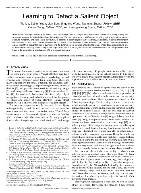
Learning to Detect a Salient ObjectTie Liu,Zejian Yuan,Jian Sun,Jingdong Wang,Nanning Zheng,Fellow,IEEE, Xiaoou Tang,Fellow,IEEE,and Heung-Yeung Shum,Fellow,IEEE Abstract—In this paper,we study the salient object detection problem for images.We formulate this problem as a binary labeling task where we separate the salient object from the background.We propose a set of novel features,including multiscale contrast,center-surround histogram,and color spatial distribution,to describe a salient object locally,regionally,and globally.A conditional random field is learned to effectively combine these features for salient object detection.Further,we extend the proposed approach to detect a salient object from sequential images by introducing the dynamic salient features.We collected a large image database containing tens of thousands of carefully labeled images by multiple users and a video segment database,and conducted a set of experiments over them to demonstrate the effectiveness of the proposed approach.Index Terms—Salient object detection,conditional random field,visual attention,saliency map.Ç1I NTRODUCTIONT HE human brain and visual system pay more attention to some parts of an image.Visual attention has been studied by researchers in physiology,psychology,neural systems,and computer vision for a long time.There are many applications for visual attention,for example,auto-matic image cropping[1],adaptive image display on small devices[2],image/video compression,advertising design [3],and image collection browsing[4].Recent studies[5], [6],[7]demonstrated that visual attention helps object recognition,tracking,and detection as well.In this paper, we study one aspect of visual attention—salient object detection.Fig.1shows some examples of salient objects.For instance,people are usually interested in the objects in images in Fig.1,and the leaf,car,and woman attract the most visual attention in each respective image.We call them salient objects or foreground objects that we are familiar with,or objects with the most interest.In many applica-tions,such as image display on small devices[2]and image collection browsing[4],people want to show the regions with the most interest,or the salient objects.In this paper, we try to locate these salient objects automatically with the supposition that a salient object exists in an image.1.1Related WorkMost existing visual attention approaches are based on the bottom-up computational framework[8],[9],[10],[11],[12], [13],[14],[15],[16],where visual attention is supposed to be driven by low-level stimulus in the scene,such as intensity, contrast,and motion.These approaches consist of the following three steps:The first step is feature extraction in which multiple low-level visual features,such as intensity, color,orientation,texture,and motion,are extracted from the image at multiple scales.The second step is saliency computation.The saliency is computed by a center-surround operation[13],self-information[8],or graph-based random walk[9]using multiple features.After normalization and linear/nonlinear combination,a master map[17]or a saliency map[14]is computed to represent the saliency of each image st,a few key locations on the saliency map are identified by winner-take-all,or inhibition-of-return,or other nonlinear operations.Recently,a saliency model based on low,middle,and high-level image features was trained using the collected eye tracking data[18].While these approaches have worked well in finding a few fixation locations in synthetic and natural images,they have not been able to accurately detect where the salient object should be.For instance,the middle row in Fig.1shows three saliency maps computed using Itti’s algorithm[13].Note that the visual saliency concentrates on several small local regions with high-contrast structures,e.g.,the background grid in Fig.1a,the shadow in Fig.1b,and the foreground boundary in Fig.1c.Although the leaf in Fig.1a commands much attention,the saliency for the leaf is low.Therefore, these saliency maps computed from low-level features don’t have the notation of objects,and they are not good indications for where a salient object is located while perusing these images.Figure-ground segregation is somehow related to salient object detection.However,the usually figure-ground.T.Liu is with the Institute of Artificial Intelligence and Robotics,Xi’anJiaotong University,and the Analytics and Optimization Department,IBM Research-China,Building19A2F,Zhongguancun Software Park,8Dongbeiwang West Road,Haidian District,Beijing100193,P.R.China.E-mail:liultie@..Z.Yuan and N.Zheng are with the Institute of Artificial Intelligence andRobotics,Xi’an Jiaotong University,28Xianning Xilu,Xi’an710049,China.E-mail:yzejian@,nnzheng@..J.Sun is with the Visual Computing Group,Microsoft Research Asia,5/F,Beijing Sigma Center,No.49,Zhichun Road,Haidian District,Beijing100190,P.R.China.E-mail:jiansun@..J.Wang is with the Media Computing Group,Microsoft Research Asia,5/F,Beijing Sigma Center,No.49,Zhichun Road,Haidian District,Beijing100190,P.R.China.E-mail:jingdw@..X.Tang is with the Department of Information Engineering,ChineseUniversity of Hong Kong,Shatin,Hong Kong.E-mail:xtang@.hk..H.-Y.Shum is with the On-Line Service Division,R&D,Microsoft,OneMicrosoft Way,Redmond,WA98052.E-mail:hshum@.Manuscript received4Dec.2008;revised23Oct.2009;accepted29Nov.2009;published online2Mar.2010.Recommended for acceptance by A.Torralba.For information on obtaining reprints of this article,please send e-mail to:tpami@,and reference IEEECS Log NumberTPAMI-2008-12-0834.Digital Object Identifier no.10.1109/TPAMI.2010.70.0162-8828/11/$26.00ß2011IEEE Published by the IEEE Computer Societysegregation algorithm works with the supposition of the category of objects [19],[20],[21]or with interactions [22],[23].If the object is assigned a given category,the specific features,for example,for cows,can be defined specially,and these features cannot be adopted for other categories.For interactive figure-ground segmentation,the appearance model is usually set up,where for our salient object detection,we do not have such an appearance model.Visual attention is also studied for sequential images,where the spatiotemporal cues from image sequences are indicated to be helpful for visual attention detection.For instance,motion from objects or backgrounds helps to indicate the salient fixations [24],[25],[26].Large motion [27]and motion contract [24]are supposed to induce prominent attention,ually,the visual saliency from a single image is combined with the motion saliency for better visual attention detection,and different combination strate-gies are introduced in [27].Video surprising [11]is also related,where it describes the KullbackLeibler divergence between the prior and posterior distribution of a feature map.These visual attention approaches suffer from the similar shortcoming to the visual attention approaches for single image.Automatic object discovery [28],[29],[30]deals with a similar salient object detection task for sequential images.The objects are extracted and tracked using motion-based layer segmentation in [28]and a generative model of objects by defining switch variables for combinatorial model selection is adopted in [29].The unsupervised video object discovery [30]combines the topic model and the temporal model for videos.1.2Our ApproachIn this paper,we investigate one aspect of visual attention,namely,salient object detection.We incorporate the high-level concept of the salient object into the process of saliency map computation.As can be observed in Fig.2,people naturally pay more attention to salient objects in images,such as a person,a face,a car,an animal,or a road sign.Therefore,we formulate salient object detection as a binary labeling problem that separates a salient object from thebackground.Like face detection,we learn to detect a familiar object;unlike face detection,we detect a familiar yet unknown object in an image.We present a supervised approach to learn to detect a salient object in an image or sequential images.First,we model the salient object detection problem by a condition random field (CRF),where a group of salient features are combined through CRF learning.Moreover,the segmenta-tion is also incorporated into the CRF to detect a salient object with unknown size and shape.The last row in Fig.1shows the saliency maps computed by our approach.Second,to overcome the challenge that we do not know what a specific object or object category is,we propose a set of novel local,regional,and global salient features to define a generic salient object.We also define the salient features on the motion field similarly to capture the spatiotemporal cues.Then,we construct a large image database with 20,000+well-labeled images for training and evaluation.To the best of our knowledge,it is the first time a large image database has been made available for quantitative evaluation.The remainder of the paper is organized as follows:Section 2introduces the formulation of the salient object detection problem,and the salient object features are presented in Section 3.Section 4introduces the image database and the evaluation experiments.Section 5dis-cusses the connections between our approach and related approaches,and the conclusion follows in Section 6.2F ORMULATIONGiven an image I ,we represent the salient object as a binary mask A ¼f a x g .For each pixel x ,a x 2f 1;0g is a binary label to indicate whether the pixel x belongs to the salient object.Similarly,the salient objects in sequential images,f I 1;...;I t ;...;I N g ,are represented by a sequence of binary masks f A 1;...;A t ;...;A N g ,with A t corresponding to image I t .In this paper,we formulate the salient object detection problem as a binary labeling task by inspecting whether each pixel belongs to the salient object.We first present the conditional random field formulation to the single-imageFig. 2.Sample images in our image database for salient objectdetection.Fig.1.Salient object detection.From top to bottom:input image with a salient object,saliency map computed by Itti’s attention algorithm (),and saliency map computed by our salient object detection approach.case,and then extend it to the sequential image case by exploring the extra temporal information.2.1Formulation of Salient Object Detection in aSingle ImageIn the CRF framework[31],the probability of a labeling configuration A¼f a x g,given the observation image I, is modeled as a conditional distribution PðA j IÞ¼1 Z expðÀEðA j IÞÞ,where Z is the partition function.Wedefine the energy EðA j IÞas a linear combination of a set of static salient features,including a number of K unary features F kða x;IÞand a pairwise feature Sða x;a x0;IÞ:EðA j IÞ¼Xx X Kk¼1k F kða x;IÞþXx;x0Sða x;a x0;IÞ;ð1Þwhere k is the weight of the k th feature and x;x0are two adjacent pared with Markov random field,one of the advantages of CRF is that the features F kða x;IÞand Sða x;a x0;IÞcan be arbitrary low-level or high-level features extracted from the whole image.CRF also provides an elegant framework to learn an optimal combination of multiple features.Salient object feature.F kða x;IÞindicates whether a pixel x belongs to the salient object.In the next section,we propose a set of local,regional,and global salient object features.The salient object feature F kða x;IÞis formulated from a normalized feature map f kðx;IÞ2½0;1 for every pixel,and is written as follows:F kða x;IÞ¼f kðx;IÞ;a x¼0;1Àf kðx;IÞ;a x¼1:&ð2ÞPairwise feature.Sða x;a x0;IÞexploits the spatial rela-tionship between two adjacent pixels.Following the contrast-sensitive potential function in interactive image segmentation[22],we define Sða x;a x0;IÞasSða x;a x0;IÞ¼j a xÀa x0jÁexpðÀ d x;x0Þ;ð3Þwhere d x;x0¼k I xÀI x0k2is the L2-norm of the color differ-ence, is a robust parameter that weights the color contrast and can be set as ¼ð2hk I xÀI x0k2iÞÀ1[32],with hÁi being the expectation operator.This feature function can be viewed as a penalty term when adjacent pixels are assigned with different labels.The more similar the colors of the two pixels are,the less likely it is that they are assigned different labels.2.2Formulation of Salient Object Detection inSequential ImagesWe exploit the extra temporal cues to formulate salient object detection in sequential images.Besides the static salient features from a single image,the temporal features,called dynamic features,are further defined.Differently from previous work[24],[25],[26],we propose new dynamic features and learn a CRF model to combine the dynamic features and static features.Instead of building a complex3D graph formulation,e.g.,a large graph in interactive video cutout[33],[34],we integrate the cues from multiple images into a2D graph for effective and efficient optimization.Given the sequential images f I t g,t2f1;...;N g,the probability of the sequential binary maps,f A t g, t2f1;...;N g,can be modeled as a conditional distribution:PðA1;...;N j I1;...;NÞ¼1ZexpðÀEðA1;...;N j I1;...;NÞÞ;ð4Þwhere Z is the partition function.A reasonable supposition is that the salient object detection A t can be inferred from the associated frame I t and the previous frame I tÀ1.Then, the energy function EðA1;...;N j I1;...;NÞcan be decomposed as EðA1;...;N j I1;...;NÞ¼X Nt¼1EðA t j I1;...;NÞ¼X Nt¼1EðA t j I tÀ1;I tÞ:ð5ÞHere,EðA t j I tÀ1;I tÞis composed of a static term and a dynamic term.The static term is the same as the single-image case.In the dynamic term,we compute a motion field M t from a pair of successive images I tÀ1and I t,and build salient features from the motion field,and in addition, introduce an appearance coherent feature between the salient objects in the successive frames.Specifically,the energy EðA t j I tÀ1;I tÞis formulated as a linear combination of static salient features F kða x;I tÞ,a pairwise feature Sða x;a x0;IÞ,and a set of dynamic salient features,including motion salient features F kða x;M tÞand appearance coherent features F kða x;I tÀ1;I tÞ:EðA t j I tÀ1;I tÞ¼XxX Kk¼1k F kða x;I tÞþXKþLk¼Kþ1k F kða x;M tÞþ 0Fða x;I tÀ1;I tÞ!þXx;x0Sða x;a x0;I tÞ;ð6Þwhere f k g are the weights of the features,M t is the motion field corresponding to image I t,and x;x0are two adjacent pixels in image I t.F kða x;I tÞare the static salient features,and Sða x;a x0;I tÞdescribes the spatial relationship between two adjacent pixels.These two categories of features are defined as in(1).Differently from(1),more features from the temporal information are included.These are the motion salient features F kða x;M tÞfrom the motion field M t and the appearance coherent feature Fða x;I tÀ1;I tÞbetween the salient objects from two adjacent frames.Motion salient feature.F kða x;M tÞis defined,similarly to(2),as the indicator of a normalized feature mapf kðx;M tÞ2½0;1 ,where M t is the motion field of the image I t and obtained based on the SIFT flow technique[35].Appearance coherent feature.Fða x;I tÀ1;I tÞmodels the appearance coherence of the salient objects from two adjacent frames,which is defined as an indicator of a normalized feature map fðx;I tÀ1;I tÞ2½0;1 ,similarly to(2). This feature function fðx;I tÀ1;I tÞpenalizes the pixels that are identified to be in the salient object,but with a large color difference between the surrounding regions from two adjacent frames.With this appearance coherent feature,the salient objects from two adjacent frames can be labeled more consistently.2.3Learning and Inference for The CRF ModelThe objective functions of the salient object detection for single-image and sequential-image cases in(1)and(6)are essentially very similar to the perspective of the CRF formulation,i.e.,a linear combination of a set of features.To get the linear combination of features,the goal of CRFLIU ET AL.:LEARNING TO DETECT A SALIENT OBJECT355learning is to estimate the linear weights !¼f k g under the Maximized Likelihood (ML)criteria.In the following,we present the parameter learning scheme for the single-image case.The parameter learning scheme for the sequential image case can be similarly obtained.Given N training image pairs f I n ;A n g N n ¼1,the optimal parameters maximize the sum of the log-likelihood:Ã!¼arg max !X n log P ðA n j I n ; !Þ:ð7ÞThe derivative of the log-likelihood with respect to the parameter k is the difference between two expectations:d log P ðA n j I n ; !Þd k¼<F k ðA n ;I n Þ>P ðA n j I n ; !ÞÀ<F k ðA n ;I n Þ>P ðA n j G n Þ:ð8ÞThen,the gradient descent direction isÁ k /X nX x;a n xÀF k Àa n x ;I nÁp Àa n x j I n ;!ÁÀF k Àa n x ;I n Áp Àa n x j g n xÁÁ;ð9Þwhere p ða n x j I n ; !Þ¼R A n n a n xP ðA n x j I n ; !Þis the marginal dis-tribution and p ða n x j g n x Þis from the labeled ground truth g n x andis defined asp Àa n x j g n x Á¼1Àg n x ;a x ¼0;g nx ;a x ¼1:&ð10ÞExact computation of marginal distribution p ða n x j I n ; !Þisintractable.However,the pseudomarginal (belief)com-puted by belief propagation can be used as a good approximation [36],[19].The tree-reweighted belief propa-gation [37]can be run under the current parameters in each step of gradient descent to compute an approximation ofthe marginal distribution p ða n xj I n ; !Þ.When the combination parameters of salient features are learned,we can infer the most probable labeling A to minimize the energy from (1)and (6).We still apply the tree-reweighted belief propagation to infer the label using the learned parameters,and we will discuss the details of implementations in Section 4.3S ALIENT O BJECT F EATUREIn this section,we instantiate the formulation of salient object detection by presenting the salient object features:static salient features for the single-image case and dynamic salient features specifically for the sequential images.3.1Static Salient FeatureWe introduce local,regional,and global features that define a salient object.Since the scale selection is one of the fundamental issues in feature extraction,we resize all images so that the max(width,height)of the image is 400pixels.In the following,all parameters are set with respect to this basic image size.3.1.1Multiscale ContrastContrast is the most commonly used local feature for attention detection [13],[38],[39]because the contrast operator simulates the human visual receptive fields.With-out knowing the size of the salient object,contrast is usually computed at multiple scales.In this paper,we simply define the multiscale contrast feature f c ðx;I Þas a linear combina-tion of contrasts in the Gaussian image pyramid:f c ðx;I Þ¼X L l ¼1X x 02N ðx Þk I l ðx ÞÀI l ðx 0Þk 2;ð11Þwhere I l is the l th-level image in the pyramid and the number of pyramid levels L is 6.N ðx Þis a 9Â9window.The feature map f c ðÁ;I Þis normalized to a fixed range ½0;1 .An example is shown in Fig. 3.Multiscale contrast highlights the high-contrast boundaries by giving low scores to the homogenous regions inside the salient object.3.1.2Center-Surround HistogramAs shown in Fig.2,the salient object usually has a larger extent than local contrast and can be distinguished from its surrounding context.Therefore,we propose a regional salient feature.Suppose the salient object is enclosed by a rectangle R .We construct a surrounding contour R S with the same area of R ,as shown in Fig.4a.To measure how distinct the salient object in the rectangle is with respect to its surroundings,we can measure the distance between R and R S using various visual cues such as intensity,color,and texture/texton.In this paper,we use the 2distance between histograms ofRGB color: 2ðR;R S Þ¼12P ðR i ÀR i S Þ2i iS.We use histograms because they are a robust global description of appearance.They are insensitive to small changes in size,shape,and viewpoint.Another reason is that the histogram of a rectangle with any location and size can be very quickly computed by means of an integral histogram introduced recently [40].Fig.4a shows that the salient object (the girl)is most distinct using the 2histogram distance.We have also tried the intensity histograms and histograms of oriented gradient [41].We found that the former is redundant with the color histogram and the latter is not a good measurement because the texture distribution in a semantic object is usually not coherent.To handle varying aspect ratios of the object,we use five templates with different aspect ratios f 0:5;0:75;1:0,1:5;2:0g .356IEEE TRANSACTIONS ON PATTERN ANALYSIS AND MACHINE INTELLIGENCE,VOL.33,NO.2,FEBRUARY2011Fig.3.Multiscale contrast.From left to right:input image,contrast maps at multiple scales,and the feature map from linearly combining the contrasts at multiple scales.We find the most distinct rectangle,R Ãðx Þ,centered at each pixel x by varying the size and aspect ratio:R Ãðx Þ¼arg max R ðx Þ2ðR ðx Þ;R S ðx ÞÞ:ð12ÞThe size range of the rectangle R ðx Þis set to ½0:1;0:7 Âmin ðw;h Þ,where w;h are the image width and height.Then,the center-surround histogram feature f h ðx;I Þis defined as a sum of spatially weighted distances:f h ðx;I Þ/Xf x 0j x 2R Ãðx 0Þgw xx 0 2ðR Ãðx 0Þ;R ÃS ðx 0ÞÞ;ð13Þwhere R Ãðx 0Þis the rectangle centered at x 0and containingthe pixel x .The weight w xx 0¼exp ðÀ0:5 À2x 0k x Àx 0k 2Þis a Gaussian falloff weight with variance 2x 0,which is set to one-third of the size of R Ãðx 0Þ.Finally,the feature map f h ðÁ;I Þis also normalized to the range ½0;1 .Fig.4b shows several center-surround feature maps.The salient objects are well located by the center-surround histogram feature.The last image in Fig.4b is an especially difficult case for color or contrast-based approaches but the center-surround histogram feature can capture the “object-level”salient region.To further verify the effectiveness of this feature,we compare the center-surround histogram distance of a randomly selected rectangle,a rectangle centered at the image center,and three user-labeled rectangles in the image.Fig.5shows the average distances on the image set A ,and this image set is introduced in Section 4.It is no surprise that the salient object has a large center-surround histogram distance.3.1.3Color Spatial DistributionThe center-surround histogram is a regional feature.Is there a global feature related to the salient object?We observe from Fig.2that the more widely a color is distributed in the image,the less possible it is that a salient object contains this color.The global spatial distribution of a specific color can be used to describe the saliency of an object.To describe the spatial distribution of a specific color,the simplest approach is to compute the spatial variance of the color.First,all colors in the image are represented by Gaussian Mixture Models (GMMs)f w c ; c ;Æc g C c ¼1,where f w c ; c ;Æc g is the weight,the mean color,and the covar-iance matrix of the c th component.Each pixel is assigned to a color component with the probability:p ðc j I x Þ¼w c N ðI x j c ;Æc ÞPcw c N ðI x j c ;Æc Þ:ð14ÞThen,the horizontal variance V h ðc Þof the spatial positionfor each color component c isV h ðc Þ¼1c Xxp ðc j I x ÞÁj x h ÀM h ðc Þj 2;ð15ÞM h ðc Þ¼1j X j c Xxp ðc j I x ÞÁx h ;ð16Þwhere x h is the x-coordinate of the pixel x andj X j c ¼Px p ðc j I x Þ.The vertical variance V v ðc Þis similarly defined.The spatial variance of a component c is V ðc Þ¼V h ðc ÞþV v ðc Þ.We normalized f V ðc Þg c to the range ½0;1 (V ðc Þ ðV ðc ÞÀmin c V ðc ÞÞ=ðmax c V ðc ÞÀmin c V ðc ÞÞ).Finally,the color spatial-distribution feature f s ðx;I Þis defined as a weighted sum:f s ðx;I Þ/Xcp ðc j I x ÞÁð1ÀV ðc ÞÞ:ð17ÞThe feature map f s ðÁ;I Þis also normalized to the range ½0;1 .Fig.6b shows color spatial-distribution feature maps of several example images.The salient objects are well covered by this global feature.Note that the spatial variance of the color at the image corners or boundaries may also be small because the image is cropped from the whole scene.To reduce this artifact,a center-weighted,spatial-variance feature is defined asLIUET AL.:LEARNING TO DETECT A SALIENT OBJECT 357Fig.5.The average center-surround histogram distance on the image set A .1.A randomly selected rectangle.2.A rectangle centered at the image center with 55percent ratioof area to image.3-5.Rectangles labeled by three users.Fig. 4.Center-surround histogram.(a)Center-surround histogram distances with different locations and sizes.(b)Top row are input images and bottom row are center-surround histogram feature maps.f s ðx;I Þ/X cp ðc j I x ÞÁð1ÀV ðc ÞÞÁð1ÀD ðc ÞÞ;ð18Þwhere D ðc Þ¼Px p ðc j I x Þd x is the weight which assigns less importance to colors nearby image boundaries and is also normalized to ½0;1 ,similarly to V ðc Þ.d x is the distance from pixel x to the image center.As shown in Fig.6c,center-weighted,color spatial variance shows a better prediction of the saliency of each color.To verify the effectiveness of this global feature,we plot the color spatial variance versus average saliency prob-ability curve on the image set A ,as shown in Fig.7.Obviously,the smaller a color variance is,the higher the probability the color belongs to the salient object is.3.2Dynamic Salient Feature3.2.1Motion Salient FeaturesThe motion field and the features derived from it are useful to induce visual attention.For example,large motion and motion contract are supposed to induce visual attention in [27],[24],and a constant velocity motion model is assumed for the salient object in [30].Motion magnitude is a possible cue,but may not be sufficient.For example,in Fig.8a,the region with larger motion magnitude includes the salient object.In contrast,the region with smaller motion magni-tude includes the salient object in Fig.8b.In this paper,we view the motion field as an image and define the local,regional,and global salient features from it.We compute the motion field M using the SIFT flow [35].It can be observed that the motion fields have some special properties for the salient feature computation.For example,the motion fields from the salient object tend to be consistent because the regions from the salient object are inclined to have a similar motion,and the motion fields in the regions of object boundaries are usually disordered.To measure this consistency,motion variance V ðx;M Þin a small rectangle surrounding x is computed,and a weight is assigned to each pixel as follows:W ðx;M Þ¼exp ðÀ c k V ðx;M Þk 2Þ;ð19Þwhere V ðx;M Þis computed on a 2D motion vector from a window (5Â5in this paper)centered at x and c ¼0:2.As in the first row of Fig.9,the motion from the surrounding region of pixel x is more cluttered and the weight of pixel x is smaller.Compared with the salient features defined for a single image,all the local,regional,and global salient features are defined similarly on weighted 2D motion vectors,including the motion magnitude and the motion direction.In the following,we present the formulation and only highlight the difference from the image:Multiscale contrast of weighted motion field.It is defined on weighted motion vectors as follows:f M c ðx;M Þ¼X L l ¼1X x 02N ðx ÞW l x W l x 0k M l ðx ÞÀM l ðx 0Þk 2;ð20Þwhere M l is the l th-level motion in the pyramid and W lx is the weight at pixel x .We also test the multiscale contrast on motion magnitude or motion direction.They do not outperform the feature on the 2D motion vector because neighborhood pixels may have the same motion magnitude358IEEE TRANSACTIONS ON PATTERN ANALYSIS AND MACHINE INTELLIGENCE,VOL.33,NO.2,FEBRUARY2011Fig.6.Color spatial-distribution feature.(a)Input images.(b)Color spatial variance feature maps.(c)Center-weighted,color spatial variance featuremaps.Fig.7.Color spatial variance (x-coordinate)versus average saliency probability (y-coordinate)on the image set A .The saliency probability is computed from the “ground truth”labeling.Fig.8.Motion map.(a)The salient object with a large motion.(b)The background with a largemotion.Fig.9.Motion salient features.From left to right:(a)Two adjacent images,the motion field,and the motion weight map;(b)the local,regional,global,and combined motion salient features.。

ansys常见运行错误及解决办法

ANSYS常见运行错误及其解决办法ESYS is not valid for line element.原因：是因为我使用LATT的时候，把“--”的那个不小心填成了“1”。

经过ANSY S的命令手册里说那是没有用的项目，但是根据我的理解，这些所谓的没有用的项目实际上都是ANSYS在为后续的版本留接口。

对于LATT，实际上那个项目可能就是单元坐标系的设置。

当我发现原因后，把1改成0——即使用全局直角坐标系，就没有WARNING了。

当然，直接空白也没有问题。

使用*TREAD的时候，有的时候明明看文件好好的，可是却出现*TREAD end-of-file in data read.后来仔细检查，发现我TXT的数据文件里，分隔是采用TAB键分隔的。

但是在最后一列后面，如果把鼠标点上去，发现数据后面还有一个空格键。

于是，我把每个列最后多的空格键删除，然后发现上面的信息就没有了。

Coefficient ratio exceeds - Check results.？这个大概是跟收敛有关，但是我找不到具体的原因。

我建立的一个桥梁分析模型，尽管我分析的结果完全符合我的力学概念判断，规律完全符合基本规律，数据也基本符合实际观测，但是却还是不断出现这个警告信息。

？*TREAD end-of-file in data readtxt中的表格数据不完整！？No *CREATE for *END.The *END command is ignored忘了写*END了吧，呵呵？Keypoint 1 is referenced by only one line.Improperly connected lineset fo r AL command两条线不共点,尝试nummrg命令。

L1 is not a recognized PREP7 command, abbreviation, or macro.This co mmand will be ignored还没有进入prep7，先：/prep7Keypoint 2 belongs to line 4 and cannot be moved关键点2属于线4，移动低级体素时先移动高级体素！Shape testing revealed that 32 of the 640 new or modified elements？violate shape warning limits.To review test results, please see the？output file or issue the CHECK command.？单元形状奇异，在我的模型中6面体单元的三个边长差距较大，可忽略该错误用命令流建模的时候遇到的The drag direction (from the keypoint on drag line 27 that is closest？to a keypoint KP of the given area 95) is orthogonal to the area？normal at that KP.Area cannot be dragged by the VDRAG command.意思是拉伸源面的法向与拉伸路径垂直，不能使用VDRAG命令出现的环境ASEL,S,LOC,Z,143e-3VDRAG,ALL, , , , , ,27本意是按位置z=143e-3位置的面，然后沿编号27的线拉伸，出错，之前用该语句没有任何问题。

学术英语写作Unit-6.Introduction

methodology reported in the paper. In sentence 10 the writer announces the findings.
9
➢Background (sentences 1-4) ➢Literature Review (sentences 5-6) ➢Unresolved Question (sentence 7) ➢The Present Paper (sentences 8-10)
In sentence 6 the writer provides a brief overview of key research projects in this area.
In sentence 7 the writer describes a gap in the research.
In sentence 8 the writer describes the paper itself. In sentence 9 the writer gives details about the
Unit 6 How to Write the Introduction
1
Teaching Procedures
1
Lead-in
2
Sample Analysis

Building a Model
4
Grammar and Writing Skills
2
Lead-in 1. What information should be contained in the Introduction?
13
➢ The Present Paper
8. The present paper presents a set of criteria for selecting such a component. 9. On the basis of these criteria it then describes the preparation of a set of polymer blends using PLA and a hydro-carbon rubber (PI). 10. This combination of two mechanistically distinct polymerizations formed a novel polymer in which the incorporation of PI significantly increased flexibility .

佩雷尔曼关于庞加莱猜想的论文0303109

The Ricci ﬂow with surgery was considered by Hamilton [H 5,§4,5]; unfortunately, his argument, as written, contains an unjustiﬁed statement (RMAX = Γ, on page 62, lines 7-10 from the bottom), which I was unable to ﬁx. Our approach is somewhat diﬀerent, and is aimed at eventually constructing a canonical Ricci ﬂow, deﬁned on a largest possible subset of space-time, - a goal, that has not been achieved yet in the present work. For this reason, we consider two scale bounds: the cutoﬀ radius h, which is the radius of the necks, where the surgeries are performed, and the much larger radius r, such that the solution on the scales less than r has standard geometry. The point is to make h arbitrarily small while keeping r bounded away from zero.
Proof. A gradient shrinking soliton gij(t), −∞ < t < 0, satisﬁes the equation

06_MIDAS GTS NX 分析手册-荷载应变

K K AAu A = FF K SF
uS
K FS u F f F u = f A = f K SS S S
(6.1.2)
in the equation above is a determined value and thus the 2nd row of the stiffness matrix does not
u uA = F u S
uF uS
(6.1.1)
: DOF without assigned specified displacement : DOF with assigned specified displacement
The stiffness matrix can also be classified and expressed using the same principle:
1.1
Structural Load Types
Table 6.1.1 Usable loads in GTS NX
Nodal force Nodal forces are the most basic loads and have 3 force component inputs and 3 moment component inputs for each node. The direction can be defined about an arbitrary coordinate system. Pressure load The pressure load is input as a distributed force form for an element face or edge. The surface pressure load is applicable for 2D or 3D elements and the edge pressure load is applicable for 1D or 2D elements. The input direction can be specified as an arbitrary coordinate axis direction, arbitrary vector direction or normal direction. Figure 6.1.1 displays the pressure load acting on various elements.

Volvo 车辆配置手册说明书

Important NotesChassis DimensionsCab Height: +39 mm for CAB-CRW.Front Axle to Back of Cab: +1258 mm for CAB-CRW, +280 mm for CAB-SSLP. D-measure includes a front clearance of 50 mm and for rigid trucks also a subframe of 120 mm.Height can vary ± 20 mm for leaf and ± 10 mm for air suspension.All dimensions are for unladen chassis and any tag axles down. Chassis height used: CHH-MED.Weight and dimensions are based upon the following tyres:Chassis weight includes oil, water, AdBlue, 0 litres fuel and without driver. Kerb weight can vary ± 3%.Turning diameters are theoretically calculated.Legal weights can differ from country to country.For more detailed weight information, including optional equipment weights, ask your Volvo sales contact to enter your specification into the Volvo WeightChassis Dimensions [mm]WB Wheelbase3250 3500 3800 4100 4400 4700 5000 5300 5600 5900 6200 6500A Overall Chassis Length6545 6975 7425 7955 8425 8915 9435 9915 10425 10835 11430 11730 D Center of rear axle to front of body 2662 2912 3212 3512 3812 4112 4412 4712 5012 5312 5612 5912 N Rear Overhang (Min.) 1515 1685 1615 1515 1615 1615 1615 1615 1615 1615 1615 1615 NRear Overhang (Max.)19752155230525352705289531153295 3505 3615 3910 3910Y Center of Gravity for Payload (Min.) 550 594 645 699 751 802 855 905 958 1007 1060 1105 Y Center of Gravity for Payload (Max.) 748 807 877 950 1021 1092 1164 1234 1305 1374 1447 1512 W Body Length (Min.) 3829 4210 4669 5124 5581 6041 6497 6957 7414 7876 8330 8800 W Body Length (Max.) 4224 4637 5134 5627 6121 6619 7114 7613 8109 8610 9103 9614Chassis Weights [kg]Front Axle 3150 3150 3160 3155 3155 3160 3160 3170 3170 3180 3180 3200 Rear Axle 1335 1365 1400 1425 1445 1470 1495 1530 1550 1570 1595 1615 Kerb Weight4485 4515 4560 4580 4600 4630 4655 4700 4720 4750 4775 4815 Payload (including body, driver, fuel, etc.) 11515 11485 11440 11420 11400 11370 11345 11300 11280 11250 11225 11185Turning Diameter [mm]Turning Circle Diameter Kerb to Kerb 11600 12400 13300 14200 15100 16000 16900 1780018700 19600 20500 21400 Turning Circle Diameter Wall to Wall 1290013700 1460015500 16400 17300 18200 19100 20000 20900 21800 22700Plated Weights [kg]DesignGross Vehicle Weight16000 Gross Combination Weight 21000 Front Axle 5800 Rear Axle 10900■ Standard Equipment □ Optional EquipmentFor more detailed information about cab and powertrain equipment, please refer to separate specification sheets.For all possible options and combinations of options please consult your Volvo sales contact who can create a specification to match your requirements using the Volvo Sales Support system (VSS).□ GARB-PRE Garbage vehicle preparation ■ UNIFORM Basic platform vehicleCore components □ CHH-HIGH Chassis height high - approx. 1000 mm above ground level ■ CHH-MED Chassis height medium - approx. 900 mm above ground level ■ RAD-L80 Rear leaf suspension, 1 axle - 1 driven (80 mm wide leafs) □ CAB-CRW Crew cab □ CAB-DAY Day cab □ CAB-SSLP Comfort cab ■ EU6SCR Euro 6 emission level with Selective Catalytic Reduction(SCR), particle filter and Exhaust Gas Recirculation (EGR)■ D8K250 Six cylinder diesel engine, 7.7 litre Euro 6 SCR + EGR (DieselParticulate Filter), 250 hp, 950 Nm□ D8K280 Six cylinder diesel engine, 7.7 litre Euro 6 SCR + EGR (DieselParticulate Filter), 280 hp, 1050 Nm□ AL306 Automatic 6-speed Allison gearbox, max input torque 1695 Nm □ ATO1056 I-Sync, Automated manual 6 speed gearbox, 1070 Nm ■ ZTO1006 Overdrive 6 speed manual ZF gearbox, 1050 Nm □ EBR-CEB Engine compression and exhaust brake ■ EBR-EPG Engine brake with Exhaust pressure governor, EPG■ RSS1125A Rear single reduction solo axle - axle load 11 tonnes, GCW 25tonnes□ RSS1132A Rear single reduction solo axle - axle load 11 tonnes, GCW32.5 tonnesPackages □ DRIVEFL Driver convenience package FL □ VISIFL Visibility package FL - Optimizing the drivers field of visionaround the cab□ AIRFLOW Airflow package FL - Includes adjustable roof spoiler, sidedeflector and sun visor□ AUDIODAB Audio System DAB ■ AUDIOPD Audio Preparation DAB kit, incl. DAB-amplifier Chassis ■ FST-PAR Front parabolic leaf suspension (normal stiffness) □ FST-PAR3 Two-leaf front parabolic suspension (stiffer than normal) ■ FAL5.8 Front axle load 5.8 tonnes □ FAL6.3 Front axle load 6.3 tonnes ■ RAL10.9 Rear axle load 10.9 tonnes ■ RSTAB1 Rear stabilizer with normal stiffness □ EBS-MED EBS (Electronic Brake System) medium package ■ EBS-STD EBS (Electronic Brake System) standard package■ RST-PAR1 Rear parabolic leaf suspension□ RST-PAR3 Three leaf parabolic rear suspension, stiffer than normal□ RST-PAR4 Short four leaf parabolic rear suspension with normal stiffness ■ FST7070 Frame section thickness - web 7.0 mm / flange 7.0 mm □ FST8080 Frame section thickness - web 8.0 mm / flange 8.0 mm ■ 2BATT170 Batteries 2x170 Ah □ ADR2 ADR adaptation, 1 switch in dashboard, 1 outside on back ofcab■ R80P Right 80 litre plastic diesel tank Min volume 80l Max volume 430l ■ UL-FUEL Without left diesel tank Min volume 80l Max volume 215l □ ADTP-L AdBlue tank on left hand side ■ ADTP-R AdBlue tank on right hand side ■ WHC-FIX1 One fixed wheel chock□ TOWMBRH High mounted towing member, in centre of frame□ C-RO40AG Towing coupling Rockinger 400 G-145■ TOWF-NO1 One front towing device □ TOWF-NO2 Two front towing devices□ TOWR-ONE One rear towing device in frame end cross member□ TREL15 15 pol electrical trailer connector (ADR certified)□ TBC-EC Trailer brake connection, European Community□ RUP-FIX2 Fixed rear underrun protection, EC approved■ RFEND-T Transport mounted one-piece rear fenders□ 2024GSR General safety regulations 2024Rims and tyres □ RT-AL Brushed aluminium rims with std holes (long stud fixing) on allaxles□ RT-ALDP Dura-Bright polished aluminium rims with std holes (long studfixing) on all axles■ RT-STEEL Steel rims on all axles ■ SPWT-F Spare wheel with tyre equal to front wheel □ SWCP-LF Spare wheel carrier on left side in front of rear axle □ SWCP-R Spare wheel carrier transport mounted behind rear axle, onright-hand side (FH, FM)/below frame (FL,□ SWCP-T Spare wheel transport mounted on top of frame ■ SWCP-TP Spare wheel carrier transport mounted with the spare wheel ontop of the frame rails□ JACK-10T Jack, 10 tonnes ■ JACK-8T Jack, 8 tonnes□ GAUGE-TP Tyre pressure gaugePowertrain equipment ■ CS39A-O Single plate clutch, plate diameter 395 mm □ RET-TPT Retarder for hydraulic gearbox □ TC-HWO Oil cooler for hydraulic transmissions – water/oil■ 1COMP500 Single cylinder air compressor 360 cc / 500 l/min □ 2COM1080 Dual cylinder air compressor 720 cc / 1080 l/min ■ AIRIN-HI High air intake □ AIRIN-RL Low air intake, chassis mounted behind cab on left hand side ■ ACL1ST Air cleaner with one filter element □ ACL1ST-S Air cleaner with additional filter element ■ 24AL110B Alternator 110 Ampere □ 24AL130B Alternator 130 Ampere □ CCV-C Closed crankcase ventilation ■ CCV-OX Open crankcase ventilation with oil separator and amaintenance free gas centrifuge■ EST-AID Engine start pre-heating element □ PTER-100 Rear engine mounted clutch independent power-take-off withflange connection (DIN 100 / ISO 7646)□ PTER-DIN Rear engine mounted clutch independent PTO with splinedshaft groove (female) for a close coupled pump (DIN 5462 / ISO 7653)□ PTER1400 Rear engine mounted clutch independent power-take-off withflange connection (SAE 1410 / ISO 7647)□ PR-HF4S PTO transmission, Hydrocar, flange connection, side mounted □ PR-HF4SH PTO transmission, Hydrocar, flange connection, side mounted,high speed□ PR-HF6S PTO transmission, Hydrocar, flange connection, side mounted □ PR-HP4S PTO transmission, Hydrocar, pump connection, side mounted □ PR-HP4SH PTO transmission, Hydrocar, pump connection, side mounted,high speed□ PR-HP6S PTO transmission, Hydrocar, pump connection, side mounted □ PTR-FH1 Rear gearbox mounted Hydrocar S81 PTO with flangeconnection (DIN 90 / ISO 7646) for propeller shaft (800 Nm)connection (DIN 90 / ISO 7646) for propeller shaft (430 Nm)□ PTR-FH5 Rear gearbox mounted Hydrocar S88 PTO with flangeconnection (DIN 90 / ISO 7646) for propeller shaft (450 Nm)□ PTR-PH1 Rear gearbox mounted Hydrocar S81 PTO with connection(DIN 5462 / ISO 7653) for pump (800 Nm)□ PTR-PH2 Rear gearbox mounted Hydrocar S84 PTO with connection(DIN 5462 / ISO 7653) for pump (430 Nm)□ PTR-PH4 Rear gearbox mounted Hydrocar S88 PTO with connection(DIN 5462 / ISO 7653) for pump (450 Nm)□ PTR-PK Electrical and solenoid prep kit for gearbox PTO□ PTR-ZF2 Rear gearbox mounted ZF PTO with flange connection (DIN100 / ISO 7646) for prop shaft (410 Nm)□ PTR-ZF3 Rear gearbox mounted ZF PTO with connection (DIN 5462 /ISO 7653) for pump (410 Nm)□ PTR-ZF4 Rear gearbox mounted ZF PTO with flange connection (DIN100 / ISO 7646) for prop shaft (320 Nm)□ PTR-ZF5 Rear gearbox mounted ZF PTO with connection (DIN 5462 /ISO 7653) for pump (320 Nm)□ PTR-ZF6 Rear gearbox mounted ZF PTO with flange connection (DIN100 / ISO 7646) for prop shaft (270 Nm)□ HPG-F101 Gearbox mounted hydraulic pump F1-101, fixed displacement,single flow□ HPG-F41 Gearbox mounted hydraulic pump F1-41, fixed displacement,single flow□ HPG-F51 Gearbox mounted hydraulic pump F1-51, fixed displacement,single flow□ HPG-F61 Gearbox mounted hydraulic pump F1-61, fixed displacement,single flow□ HPG-F81 Gearbox mounted hydraulic pump F1-81, fixed displacement,single flow□ ETC Electronic throttle control - dash mounted switch for PTOspeed controlCab interior■ TAS-DIG4 Gen 4 one day digital tachograph, EC approved (GNSS &DSRC, EU 2020/1054)□ SPDU-R Dual speed limiter for rear refuse body stepsCab exterior□ SUNV-B Exterior transparent dark grey front sun visor■ SUNV-PK Exterior front sun visor installation preparation kit (fasteners)□ AD-SIDES Short cab side air deflectors□ BEACON-P Prepared for roof beacons□ BEACONA2 2 amber beacon, roof mounted warning lampsSuperstructure preparations□ FBA-BTF Front body attachments for flexible body□ FBA-BTSF Front body attachments for semi-flexible body□ RBA-T2 Rear body attachments for helper frame□ TAILPREP Tail lift preparation kitServices□ TGW-4G Telematics gateway with 4G modem■ WVTA Whole Vehicle Type Approved■ Standard Equipment □ Optional EquipmentFor more detailed information about cab and powertrain equipment, please refer to separate specification sheets.For all possible options and combinations of options please consult your Volvo sales contact who can create a specification to match your requirements using the Volvo Sales Support system (VSS).。

1、下载文档前请自行甄别文档内容的完整性，平台不提供额外的编辑、内容补充、找答案等附加服务。
2、"仅部分预览"的文档,不可在线预览部分如存在完整性等问题,可反馈申请退款(可完整预览的文档不适用该条件!)。
3、如文档侵犯您的权益，请联系客服反馈,我们会尽快为您处理(人工客服工作时间：9:00-18:30)。

LCIS - A Preview
▪ “Mathematically mimic a well-known artistic technique for rendering high contrast scenes”
▪ Coarse-to-fine rendering of boundaries and shading
▪ Constant conductivity repeated convolution with a Gaussian filter (isotropic diffusion)
Anisotropic Diffusion, cont’d
Conductivity depends on image - as local “edginess” increases, conductivity decreases
LCIS Hierarchy
(Rin,Gin,Bin)
Convert
log(L)
LCIS K0 = 0
LCIS K1
LCIS K2
LCIS K3
log(R/L,G/L,B/L)
wcolor
(Rout,Gout,Bout)
exp()
w0
w1
w2
w3
+
+
+
F = (Ixxx + Iyyx, Ixxy + Iyyy) ▪ C: Conductivity
C(x,y,t) = g(0.5(I2xx + I2yy) + I2xy)
LCIS - Implementation
▪ Discrete images, so quantities are approximate, based on 4-connected neighbors and a constant time step
Motivation
▪ Simple scene intensity adjustment Id = F(m·Is)
Id: display intensity Is: scene intensity m: scale factor
: compression/expansion term
F: enforces boundary conditions
Motivation
▪ Detail visible almost everywhere in a scene ▪ Difficult to capture rich detail in high-
contrast scenes ▪ CRT contrast: 100:1 ▪ Target scene contrast: ~100,000:1
▪ 3rd order derivatives instead of 2nd order ▪ Equalize curvature rather than intensity
It(x,y,t) = ·(C(x,y,t)F(x,y,t)) ▪ F: motive force from high to low curvature
C(x,y,t) = g(||I||) where
g(m) = (1+(m/K)2)-1 K is a conductance threshold for m
Anisotropic Diffusion Illustrated
LCIS vs. Anisotropic Diffusion
LCIS - Theory
LCIS - A Preview
▪ Low Curvature Image Simplifier ▪ Hierarchy of sharp boundaries and smooth
shadings ▪ Goal - low contrast, highly detailed images
LCIS vs. Linear Filter Hierarchies
Anisotropic Diffusion
▪ Treat intensity as heat fluid ▪ Temperature wants to flow from hot to cold
It = ·(C(x,y,t) I)
• It : derivative of temperature change w.r.t. time • C : Conductivity
LCIS: A Boundary Hierarchy For Detail-Preserving Contrast Reduction
Jack Tumblin and Greg Turk
Georgia Institute of Technology SIGGRAPH 2019
Presented by Rob Glaubius