最小费用最大流问题matlab程序
求解最大流问题的matlab程序(Matlab program for solving maximum flow problems)
求解最大流问题的matlab程序(Matlab program for solvingmaximum flow problems)Maximum flow algorithmAlgorithm idea: the maximum flow problem is actually a feasible flow {fij}, which makes the V (f) reach the maximum. If you give a feasible flow F, as long as there is no judgment in N augmenting path on the F, if there is an augmented path, improved F, a new feasible flow rate increases; if there is no augmenting path, get the maximum flow.1. labeling method for maximum flow (Ford, Fulkerson)Starting with a feasible flow (a general zero flow), the following labeling procedure and the adjustment process are followed until no augmenting path about F can be found.(1) labeling processIn this process, the points in the network are divided into labeled and unlabeled points, and the labeled points are divided into two kinds: checked and unchecked. Each label label information points are expressed in two parts: the first label show that the label from which point to start the traceback path from the VT to find out is augmented; second label is said to have checked whether the vertex.At the start of the label, mark vs (s, 0), when vs is the label, but at the end of the check point, and the rest are unlabeled points, denoted as (0, 0).Take a label without checking the point VI, for all unlabeled points, vj:A. for arc (VI, VJ), if fij<cij, then give the VJ label (VI,0), then the VJ point becomes the label, which is not checked.B. for arc (VI, VJ), if fji>0, then give the VJ label (-vi, 0), then the VJ point becomes the label, which is not checked.Thus, VI becomes a labeled and checked point, and its second label is denoted as 1. Repeat the steps above and, once VT is marked, indicate an extended path from VI to P, and VT into the adjustment process.If all the labels have been checked and the label process fails, the algorithm ends with the feasible flow being the maximum flow.(2) adjustment processFrom the VT point, through the first label of each point, backward tracing, we can find the augmenting path P. For example, if the first label of VT is VK (or -vk), then the arc (VK, VT) (or correspondingly (VT, VK)) is the arc on the P. Next, check the first label of VK, and if it is VI (or -vi), find (VI, VK) (or VI (VK)). Check the first label of VI, and so on, until vs. At this point, the entire augmenting path is found. Calculate the Q at the same time as you look for the augmenting path:Q=min{min (cij-fij), minf*ij}Convective f is subject to the following modifications:F'ij = fij+Q (VI, VJ) set prior to the arc in P'sF'ij = fij-Q (VI, VJ) and P to arc setF'ij = f*ij (VI, VJ) does not belong to the set of PNext, all tags are cleared and the new feasible stream 'f' is re entered into the labeling process.Matlab procedures for solving the maximum flow problem. (2007-05-22 19:41:06) reprint label: maximum flow problem matlabCall way: need to be abstracted into graph matrix, abstract methods: (I, J, C, f) i--- nock, j--- arrow, c---v (I, J) the capacity of f---v (I, J) of the flow.main programFunction R=maxliu (R)While (1)VV=zengguang (R);If VV==inf return; endR (VV (1), 4) =R (VV ((1)) 4) +VV ((2) *min) (VV ((:: 3));EndThe outer function 1, the expansion matrix of the graph RFunction VV=zengguang (R)% for the shortest extension chain, requiring labeling, starting at 1, and ending at the maximumK=size (R, 1);N=max (R ((:: 2));B=R (:: 1:2);For i=1:k;A (I, 1) =R (I, 3) -R (I, 4);If R (I, 1) ~=1&&R (I, 2) ~=n;A (I, 2) =R (I, 4);ElseA (I, 2) =0;EndEndR=1;For i=1:nFor j=1:kIf (A (J, 1) (~=0) and B (J, 1) ==i) V (R::) =[i, B (J, 2)];r = r + 1.endif (i) = 0) & & (b, i, 2) = = 1)v (r) = (1, b), (d) (1);r = r + 1.endendendp = zeros (n, n).for i = 1: size (v, 1)p (v (i, 1), v (i, 2)) = 1.endq = dijkstra (p, 1, n).if q = inf (vv = inf); return; end for i = 1: length (q) (1).pi = (q (1, i), q (1, i + 1)];r1 = find (b (1) = p (1));r2 = find (b (2) = p (1));rr = intersect (r1, r2).d = 1.the isempty() (rr)r1 = find (b (1) = p (1));r2 = find (b (2) = p (1));rr = intersect (r1, r2).d = - 1.end(i) = rr.- (i) = -.endfor i = 1: size (vv. 1)if it (i) = = 1)aa (i, 1) = ((i, 1), (1);endif it (i) = = 1)aa (i, 1) = ((i, 1), (2);endend(:, 2) = tt.vv: (3) = sa;外部函数2, dijkstra方法求最段路. the foot = dijkstra (v, x, y)% 正权数m = size (v, 1).t = zeros (m, 1);% t的初始化 inft = t ^ - 1.dml =;% lmd的初始化 infp = t;% p的初始化 infs = zeros (n, 1);% s的初始化 (进入s集的点为1)s (x) = 1);% 根据本题已知的初始化p (x) = 0 (x) = 0,; french;k = x;%%%%%%%%%%%%%%%%%%%%%%%%%%%%%%%%%%%%%%%%%%%%%%%%%%%%%%%%%%% %%%%%%%%%%%%%%%%%%%%%%%%%%%%%%%%%%%%%%%%%%%%%%%%%%%%%%%%%%% %%%%%%%%%%%%%%%%%%%%%%%%%%%%%%%%%%%%%%%%%%%%%%%%%%%%%%%%%%% %%%%%%%%%%%%%%%%%%%%%%%%%%%%%%%%%%%%%%%%%%%%%%%%%%%%%%%%%%% %%%%%%%%%%%%%%%%%%%%%%%%%%%%%%%%%%%%%%%%%%%%%%%%%%%%%%%%%%% %%%%%%%%%%%%%%%%%%%%%%%%%%%%%%%%%%%%%%%%%%%%%%%%%%%%%%%%%%% %%%%%%%%%%%%%%%%%%%%%%%%%%%%%%%%%%%%%%%%%%%%%%%%%%%% 计算 p"(1)a = find (s = 0).aa = find (s = 1).the size (a, 1) = mbreak;endfor i = 1: size (a, 1)pi = (i, 1).if v (k, l) = 0.if t (pp) (p (k) + v (k, l). (p) = (p (k) + v (k, l).dml (pi) = k;endendendmi = min (t (a));if mi = infbreak;elsed = find (t = e).d = d (1);p (d) = mi.(d) = inf, 为了避免同样的数字出现两次. k = d(d) = 1.endendthe mdl (y) = inffoot = inf.return;endfoot (1).g = 2; m = y;"(1)if h = x x x x x x xbreak;endfrench football (g) = (h).g = g + 1.h = (h); mdlendpace = foot);for i = 1: length (foot)foot (1, i) = (1) / length (foot) + 1 (i). end。
最小费用最大流问题matlab程序
下面的最小费用最大流算法采用的是“基于Floyd最短路算法的Ford和Fulkerson迭加算法”,其基本思路为:把各条弧上单位流量的费用看成某种长度,用Floyd求最短路的方法确定一条自V1至Vn的最短路;再将这条最短路作为可扩充路,用求解最大流问题的方法将其上的流量增至最大可能值;而这条最短路上的流量增加后,其上各条弧的单位流量的费用要重新确定,如此多次迭代,最终得到最小费用最大流。
本源码由GreenSim团队原创,转载请注明function [f,MinCost,MaxFlow]=MinimumCostFlow(a,c,V,s,t)%%MinimumCostFlow.m% 最小费用最大流算法通用Matlab函数%% 基于Floyd最短路算法的Ford和Fulkerson迭加算法% GreenSim团队原创作品,转载请注明%% 输入参数列表% a 单位流量的费用矩阵% c 链路容量矩阵% V 最大流的预设值,可为无穷大% s 源节点% t 目的节点%% 输出参数列表% f 链路流量矩阵% MinCost 最小费用% MaxFlow 最大流量%% 第一步:初始化N=size(a,1);%节点数目f=zeros(N,N);%流量矩阵,初始时为零流MaxFlow=sum(f(s,:));%最大流量,初始时也为零flag=zeros(N,N);%真实的前向边应该被记住for i=1:Nfor j=1:Nif i~=j&&c(i,j)~=0flag(i,j)=1;%前向边标记flag(j,i)=-1;%反向边标记endif a(i,j)==infa(i,j)=BV;w(i,j)=BV;%为提高程序的稳健性,以一个有限大数取代无穷大endendendif L(end)<BVRE=1;%如果路径长度小于大数,说明路径存在elseRE=0;end%% 第二步:迭代过程while RE==1&&MaxFlow<=V%停止条件为达到最大流的预设值或者没有从s到t的最短路%以下为更新网络结构MinCost1=sum(sum(f.*a));MaxFlow1=sum(f(s,:));f1=f;TS=length(R)-1;%路径经过的跳数LY=zeros(1,TS);%流量裕度for i=1:TSLY(i)=c(R(i),R(i+1));endmaxLY=min(LY);%流量裕度的最小值,也即最大能够增加的流量for i=1:TSu=R(i);v=R(i+1);if flag(u,v)==1&&maxLY<c(u,v)%当这条边为前向边且是非饱和边时f(u,v)=f(u,v)+maxLY;%记录流量值w(u,v)=a(u,v);%更新权重值c(v,u)=c(v,u)+maxLY;%反向链路的流量裕度更新elseif flag(u,v)==1&&maxLY==c(u,v)%当这条边为前向边且是饱和边时 w(u,v)=BV;%更新权重值c(u,v)=c(u,v)-maxLY;%更新流量裕度值w(v,u)=-a(u,v);%反向链路权重更新elseif flag(u,v)==-1&&maxLY<c(u,v)%当这条边为反向边且是非饱和边时 w(v,u)=a(v,u);c(v,u)=c(v,u)+maxLY;w(u,v)=-a(v,u);elseif flag(u,v)==-1&&maxLY==c(u,v)%当这条边为反向边且是饱和边时 w(v,u)=a(v,u);c(u,v)=c(u,v)-maxLY;w(u,v)=BV;elseendendMaxFlow2=sum(f(s,:));MinCost2=sum(sum(f.*a));if MaxFlow2<=VMaxFlow=MaxFlow2;MinCost=MinCost2;[L,R]=FLOYD(w,s,t);elsef=f1+prop*(f-f1);MaxFlow=V;MinCost=MinCost1+prop*(MinCost2-MinCost1);returnendif L(end)<BVRE=1;%如果路径长度小于大数,说明路径存在elseRE=0;endendfunction [L,R]=FLOYD(w,s,t)n=size(w,1);D=w;path=zeros(n,n);%以下是标准floyd算法for i=1:nfor j=1:nif D(i,j)~=infpath(i,j)=j;endendendfor k=1:nfor i=1:nfor j=1:nif D(i,k)+D(k,j)<D(i,j)D(i,j)=D(i,k)+D(k,j);path(i,j)=path(i,k);endendendendL=zeros(0,0);R=s;while 1if s==tL=fliplr(L);L=[0,L];returnendL=[L,D(s,t)];R=[R,path(s,t)];s=path(s,t);end(此文档部分内容来源于网络,如有侵权请告知删除,文档可自行编辑修改内容,供参考,感谢您的支持)。
matlab、lingo程序代码20-最大流问题
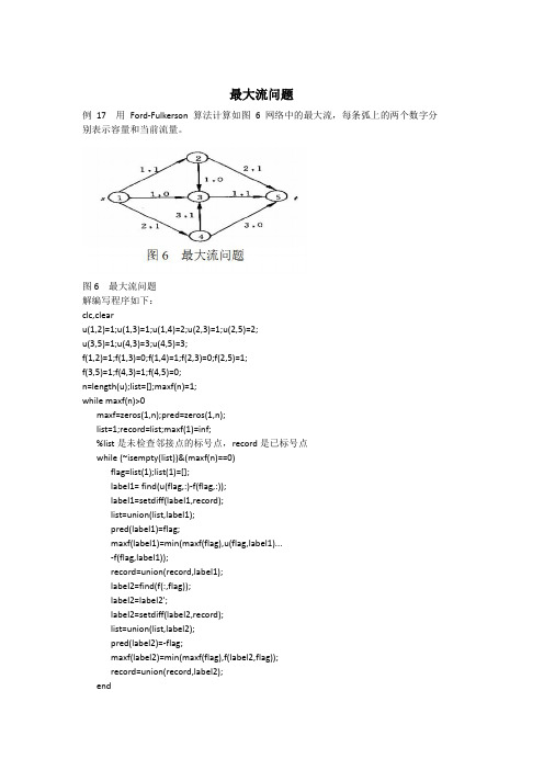
最大流问题例17用Ford-Fulkerson算法计算如图6网络中的最大流,每条弧上的两个数字分别表示容量和当前流量。
图6最大流问题解编写程序如下:clc,clearu(1,2)=1;u(1,3)=1;u(1,4)=2;u(2,3)=1;u(2,5)=2;u(3,5)=1;u(4,3)=3;u(4,5)=3;f(1,2)=1;f(1,3)=0;f(1,4)=1;f(2,3)=0;f(2,5)=1;f(3,5)=1;f(4,3)=1;f(4,5)=0;n=length(u);list=[];maxf(n)=1;while maxf(n)>0maxf=zeros(1,n);pred=zeros(1,n);list=1;record=list;maxf(1)=inf;%list是未检查邻接点的标号点,record是已标号点while(~isempty(list))&(maxf(n)==0)flag=list(1);list(1)=[];label1=find(u(flag,:)-f(flag,:));label1=setdiff(label1,record);list=union(list,label1);pred(label1)=flag;maxf(label1)=min(maxf(flag),u(flag,label1)...-f(flag,label1));record=union(record,label1);label2=find(f(:,flag));label2=label2';label2=setdiff(label2,record);list=union(list,label2);pred(label2)=-flag;maxf(label2)=min(maxf(flag),f(label2,flag));record=union(record,label2);endif maxf(n)>0v2=n;v1=pred(v2);while v2~=1if v1>0f(v1,v2)=f(v1,v2)+maxf(n);elsev1=abs(v1);f(v2,v1)=f(v2,v1)-maxf(n);endv2=v1;v1=pred(v2);endendendf最大流问题例18现需要将城市s的石油通过管道运送到城市t,中间有4个中转站321,,v v v和4v,城市与中转站的连接以及管道的容量如图7所示,求从城市s到城市t的最大流。
求网络的最小费用最大流matlab实现

<!DOCTYPE HTML PUBLIC "-//W3C//DTD HTML 4.0 Transitional//EN"><!-- saved from url=(0048)/yunyan8/shu/file/wlzxfy.htm --><HTML><HEAD><TITLE>求网络的最小费用最大流</TITLE><META http-equiv=Content-Type content="text/html; charset=gb2312"><META content="MSHTML 6.00.2800.1106" name=GENERATOR><META content=FrontPage.Editor.Document name=ProgId></HEAD><BODY background=求网络的最小费用最大流.files/bb.jpg><TABLE height=5124 cellSpacing=0 cellPadding=0 width=585 align=centerborder=0><TBODY><TR><TD width=585 height=33><P><A href="/yunyan8/shu/file/SHAI.HTM">首页</A>|<Ahref="/2/default.asp?name=yunyan8">留言</A>|<Ahref="/" target=_blank>论坛</A></P></TD></TR><TR><TD width=585 height=38><P align=center><FONT size=5><B><FONTcolor=#3366ff>求网络的最小费用最大流</FONT></B></FONT></P></TD></TR><TR><TD width=585 height=5053><FONTcolor=#3366ff>求网络的最小费用最大流,弧旁的数字是容量(运费)。
最小费用最大流算法

//此算法必须指定要求的最大流stream,如果结果无限循环的出现//一些字或者什么也不出现,则说明该图达不到此流量。
#include "iostream.h"#define max 10000#define n 5 //根据不同问题可修改大小#define stream 10 //根据不同问题可修改//最大容量矩阵intc[n][n]={{0,10,8,max,max},{max,0,max,2,7},{max,5,0,10,max},{max,max,max,0,4},{max,max,max,max,0 }};//实际流量矩阵intflow[n][n]={{0,0,0,max,max},{max,0,max,0,0},{max,0,0,0,max},{max,max,max,0,0},{max,max,max,max, 0}};//费用矩阵intmoney[n][n]={{0,4,1,max,max},{max,0,max,6,1},{max,2,0,3,max},{max,max,max,0,2},{max,max,max,ma x,0}};//增广链向量int p[n]={0,0,0,0,0}; //原点到各点的最短路径int D[n]; //原点到各点的路长(用于Dijkstra法中)int pt[n]={0,0,0,0,0}; //原点到各点的路长(用于逐次逼近法中)int maxflow; //设置最大流量//----------------------------计算Vs--Vt最短路径模块---------------------------------------------//void Dijkstra() //求源点V0到其余顶点的最短路径及其长度;得到一条增广链{int s[n]; //D[n]最后保存各点的最短路径长度int i,j,k,vl,pre;int min;int inf=20000;vl=0; //求V0到Vn的增广链for(i=0;i<n;i++){D[i]=money[vl][i]; //置初始距离值if((D[i]!=max) && (D[i]!=0)) p[i]=1;else p[i]=0;}for(i=0;i<n;i++) s[i]=0;s[vl]=1; D[vl]=0;for(i=0;i<n;i++){min=inf;for(j=0;j<n;j++)if((!s[j]) && (D[j]<min)){min=D[j];k=j;}s[k]=1;if(min==max) break;for(j=0;j<n;j++)if((!s[j]) && (D[j]>D[k]+money[k][j])){D[j]=D[k]+money[k][j];p[j]=k+1;}} //此时所有顶点都已扩充到红点集S中cout<<"Vs到Vt的最短路径为(长和径):\n";for(i=0;i<n;i++){if(i=n-1){cout<<D[i]<<" "<<i+1; //这里不需要打印pre=p[i];while (pre!=0){cout<<"<-- "<<pre; //这里不需要打印pre=p[pre-1]; //p[]中保存的路径的顶点标号从1开始,不是0;}cout<<"\n";}}}//-----------------------------------END Dijkstra()-----------------------------------------////------------------用最大流算法的方法调整实际流量矩阵flow[][],以扩充其流量----------------// void modify(){int i,min;int pre;if(D[n-1]==max){cout<<"不存在增广链";return;}pre=p[n-1];i=n-1;min=c[pre-1][i]-flow[pre-1][i]; //增广路上的最后一条边的长while(pre!=0) //再增广路上算出所能增加流量的最大值{i=pre-1;pre=p[pre-1];if(min>c[pre-1][i]-flow[pre-1][i])min=c[pre-1][i]-flow[pre-1][i];if(pre==1)pre=0;}if((min+maxflow)>stream)min=stream-maxflow;pre=p[n-1]; //在增广链上添加流量i=n-1;flow[pre-1][i]+=min;while(pre!=0){i=pre-1;pre=p[pre-1];flow[pre-1][i]+=min;if(pre==1)pre=0;}}//----------------------------------END modify()----------------------------------////--------------------------------调整费用矩阵money[][]-----------------------------// void modifymoney(){int i,j;int moneypre[n][n];for(i=0;i<n;i++)for(j=0;j<n;j++)moneypre[i][j]=money[i][j];for(i=0;i<n;i++)for(j=0;j<n;j++){if(i<j){if(c[i][j]!=max && c[i][j]>flow[i][j])money[i][j]=moneypre[i][j];if((c[i][j]!=max && c[i][j]==flow[i][j]) || (c[i][j]==max && flow[i][j]==max)) money[i][j]=max;}if(i>j){if( flow[j][i]>0 )money[i][j]=-moneypre[j][i];if(flow[j][i]==0)money[i][j]=max;}}for(i=0;i<n;i++)for(j=0;j<n;j++){if(i==j)money[i][j]=0;if(money[i][j]==-max)money[i][j]=max;}}//----------------------------------END modifymoney()----------------------------------////----------------------------采用逐次逼近法得到一条增广链----------------------------// void approach(){int pf[n],ptf[n]={0,0,0,0,0}; //当N变动时,0的个数应与N一致int min=max;int i,j,flag;for(j=0;j<n;j++)pt[j]=money[0][j]; //直接距离做初始解do{flag=1;for(j=0;j<n;j++)pf[j]=pt[j]; //将上一次得到的路径迭代结果保存入pf[]for(i=0;i<n;i++){min=pt[i];for(j=0;j<n;j++){if(min>(pt[j]+money[j][i]))min=pt[j]+money[j][i];}ptf[i]=min;}for(i=0;i<n;i++){pt[i]=ptf[i];if(pf[i]!=pt[i])flag=0; //两次迭代的值不同,继续}}while(flag==0);j=n-1;for(i=0;i<j;i++) //找出最短路径走向if(pt[i]+money[i][j]==pt[j]){p[j]=i+1; //p[j]中的下标从1开始if(p[j]==1) break;j=i;i=-1;}for(i=0;i<n;i++)D[i]=pt[i];}//------------------------------END approach()------------------------------//void main(){int i,j;Dijkstra();while( 1 ){modify(); //调整流量矩阵maxflow=0;for(j=0;j<n;j++){if(flow[0][j]!=max)maxflow+=flow[0][j];}if(maxflow==stream) break;modifymoney();approach(); //采用逐次逼近法得到一条增广链}cout<<"流量矩阵:\n";for(i=0;i<n;i++) //{for(j=0;j<n;j++)cout<<flow[i][j]<<" ";cout<<"\n";}cout<<"费用矩阵:\n";for(i=0;i<n;i++) //{for(j=0;j<n;j++)cout<<money[i][j]<<" ";cout<<"\n";}}。
实验三:使用matlab求解最小费用最大流算问题教学提纲

n=min(ta,n); %将最短路径上的最小允许流量提取出来
end
for i=1:(size(mcr',1)-1)
if a(mcr(i),mcr(i+1))==inf
a(mcr(i+1),mcr(i))=a(mcr(i+1),mcr(i))+n;
else
a(mcr(i),mcr(i+1))=a(mcr(i),mcr(i+1))-n;
if D(i,k)+D(k,j)<D(i,j)
D(i,j)=D(i,k)+D(k,j);
R(i,j)=R(i,k);
end
end
end
k;
D;
R;
end
M=D(1,n);
3.求解如下网络运输图中的最大流最小费用问题:
图2
打开matlab软件,在COMND WINDOW窗口中输入矩阵程序如下:
n=5;
新图E(f)中不考虑原网络D中各个弧的容量cij.为了使E(f)能比较清楚,一般将长度为]的弧从图E(f)中略去.由可扩充链费用的概念及图E(f)中权的定义可知,在网络D中寻求关于可行流f的最小费用可扩充链,等价于在图E(f)中寻求从发点到收点的最短路.因图E(f)中有负权,所以求E(f)中的最短路需用Floyd算法。
end
end
Mm=Mm+n; %将每次叠代后增加的流量累加,叠代完成时就得到最大流量
for i=1:size(a,1)
for j=1:size(a',1)
if i~=j&a(i,j)~=inf
if a(i,j)==A(i,j) %零流弧
c(j,i)=inf;
matlab最大流算法

matlab最大流算法摘要:一、最大流算法简介1.最大流问题的定义2.最大流算法的基本原理二、MATLAB 中的最大流算法1.MATLAB 中最大流算法的实现a.网络数据的表示b.最大流算法的实现c.结果的输出与分析三、最大流算法在MATLAB 中的实际应用1.应用背景与需求2.最大流算法的具体应用a.网络流量优化b.网络资源分配c.其他应用场景四、MATLAB 中最大流算法的优缺点分析1.优点a.高效的计算能力b.灵活的图形界面c.丰富的函数库2.缺点a.参数设置不够灵活b.算法实现不够通用c.需要较高的编程能力正文:一、最大流算法简介在网络分析中,最大流问题是一个经典的问题。
给定一个有向图G=(V,E),其中每条边(u, v) 都具有非负容量c(u, v)。
我们需要找到从源节点s 到汇节点t 的一条路径,使得该路径上的流量最大。
这就是最大流问题。
最大流算法是解决这个问题的有效方法。
最大流算法的基本原理是沿边进行松弛操作,并更新边上的流量。
当所有边的流量都达到最大值时,算法结束。
在实际应用中,最大流算法可以用于网络流量优化、网络资源分配等问题。
二、MATLAB 中的最大流算法MATLAB 提供了丰富的函数库,可以方便地实现最大流算法。
首先,我们需要用MATLAB 表示网络数据。
网络数据包括节点、边和容量信息。
我们可以用邻接矩阵或弧表来表示网络数据。
接下来,我们可以使用MATLAB 中的最大流算法求解最大流问题。
MATLAB 提供了`fmincon`函数,可以用于求解线性规划问题。
我们可以将最大流问题转化为线性规划问题,并使用`fmincon`函数求解。
最后,我们可以使用MATLAB 的图形界面功能,绘制网络图和最大流路径。
这样可以直观地展示最大流问题的解。
三、最大流算法在MATLAB 中的实际应用MATLAB 中的最大流算法可以应用于各种实际问题。
例如,在网络流量优化中,我们可以根据网络结构和流量需求,求解最大流问题,以实现流量的合理分配。
实验三:使用matlab求解最小费用最大流算问题

北京联合大学实验报告项目名称: 运筹学专题实验报告学院: 自动化专业:物流工程班级: 1201B 学号:2012100358081 姓名:管水城成绩:2015 年 5 月 6 日实验三:使用matlab求解最小费用最大流算问题一、实验目的:(1)使学生在程序设计方面得到进一步的训练;,学习Matlab语言进行程序设计求解最大流最小费用问题。
二、实验用仪器设备、器材或软件环境计算机,Matlab R2006a三、算法步骤、计算框图、计算程序等1.最小费用最大流问题的概念。
在网络D(V,A)中,对应每条弧(vi,vj)IA,规定其容量限制为cij(cij\0),单位流量通过弧(vi,vj)的费用为dij(dij\0),求从发点到收点的最大流f,使得流量的总费用d(f)为最小,即mind(f)=E(vi,vj)IA2。
求解原理。
若f是流值为W的所有可行流中费用最小者,而P是关于f的所有可扩充链中费用最小的可扩充链,沿P以E调整f得到可行流fc,则fc是流值为(W+E)的可行流中的最小费用流.根据这个结论,如果已知f是流值为W的最小费用流,则关键是要求出关于f 的最小费用的可扩充链。
为此,需要在原网络D的基础上构造一个新的赋权有向图E(f),使其顶点与D的顶点相同,且将D中每条弧(vi,vj)均变成两个方向相反的弧(vi,vj)和(vj,vi)1新图E(f)中各弧的权值与f中弧的权值有密切关系,图E(f)中各弧的权值定义为:新图E(f)中不考虑原网络D中各个弧的容量cij。
为了使E(f)能比较清楚,一般将长度为]的弧从图E(f)中略去.由可扩充链费用的概念及图E(f)中权的定义可知,在网络D中寻求关于可行流f的最小费用可扩充链,等价于在图E(f)中寻求从发点到收点的最短路.因图E(f)中有负权,所以求E(f)中的最短路需用Floyd算法。
1.最小费用流算法的框图描述。
图一2.计算最小费用最大流MATLAB源代码,文件名为mp_mc.mfunction[Mm,mc,Mmr]=mp_mc(a,c)A=a; %各路径最大承载流量矩阵C=c; %各路径花费矩阵Mm=0; %初始可行流设为零mc=0; %最小花费变量mcr=0;mrd=0;n=0;while mrd~=inf %一直叠代到以花费为权值找不到最短路径for i=1:(size(mcr’,1)—1)if a(mcr(i),mcr(i+1))==infta=A(mcr(i+1),mcr(i))—a(mcr(i+1),mcr(i)); elseta=a(mcr(i),mcr(i+1));endn=min(ta,n);%将最短路径上的最小允许流量提取出来endfor i=1:(size(mcr’,1)-1)if a(mcr(i),mcr(i+1))==infa(mcr(i+1),mcr(i))=a(mcr(i+1),mcr(i))+n;elsea(mcr(i),mcr(i+1))=a(mcr(i),mcr(i+1))—n;endendMm=Mm+n;%将每次叠代后增加的流量累加,叠代完成时就得到最大流量 for i=1:size(a,1)for j=1:size(a’,1)if i~=j&a(i,j)~=infif a(i,j)==A(i,j) %零流弧c(j,i)=inf;c(i,j)=C(i,j);elseif a(i,j)==0 %饱合弧c(i,j)=inf;c(j,i)=C(j,i);elseif a(i,j)~=0 %非饱合弧c(j,i)=C(j,i);c(i,j)=C(i,j);endendendend[mcr,mrd]=floyd_mr(c) %进行叠代,得到以花费为权值的最短路径矩阵(mcr)和数值(mrd)n=inf;end%下面是计算最小花费的数值for i=1:size(A,1)for j=1:siz e(A’,1)if A(i,j)==infA(i,j)=0;endif a(i,j)==infa(i,j)=0;endendendMmr=A—a; %将剩余空闲的流量减掉就得到了路径上的实际流量,行列交点处的非零数值就是两点间路径的实际流量for i=1:size(Mmr,1)for j=1:size(Mmr’,1)if Mmr(i,j)~=0mc=mc+Mmr(i,j)*C(i,j);%最小花费为累加各条路径实际流量与其单位流量花费的乘积endendend利用福得算法计算最短路径MATLAB源代码,文件名为floyd_mr。
- 1、下载文档前请自行甄别文档内容的完整性,平台不提供额外的编辑、内容补充、找答案等附加服务。
- 2、"仅部分预览"的文档,不可在线预览部分如存在完整性等问题,可反馈申请退款(可完整预览的文档不适用该条件!)。
- 3、如文档侵犯您的权益,请联系客服反馈,我们会尽快为您处理(人工客服工作时间:9:00-18:30)。
下面的最小费用最大流算法采用的是“基于Floyd最短路算法的Ford和Fulkerson迭加算法”,其基本思路为:把各条弧上单位流量的费用看成某种长度,用Floyd求最短路的方法确定一条自V1至Vn的最短路;再将这条最短路作为可扩充路,用求解最大流问题的方法将其上的流量增至最大可能值;而这条最短路上的流量增加后,其上各条弧的单位流量的费用要重新确定,如此多次迭代,最终得到最小费用最大流。
本源码由GreenSim团队原创,转载请注明
function [f,MinCost,MaxFlow]=MinimumCostFlow(a,c,V,s,t)
%%MinimumCostFlow.m
%最小费用最大流算法通用Matlab函数
%% 基于Floyd最短路算法的Ford和Fulkerson迭加算法
% GreenSim团队原创作品,转载请注明
%% 输入参数列表
%a单位流量的费用矩阵
%c链路容量矩阵
%V最大流的预设值,可为无穷大
%s源节点
%t目的节点
%% 输出参数列表
%f链路流量矩阵
%MinCost最小费用
%MaxFlow最大流量
%% 第一步:初始化
N=size(a,1);%节点数目
f=zeros(N,N);%流量矩阵,初始时为零流
MaxFlow=sum(f(s,:));%最大流量,初始时也为零
flag=zeros(N,N);%真实的前向边应该被记住
for i=1:N
for j=1:N
if i~=j&&c(i,j)~=0
flag(i,j)=1;%前向边标记
flag(j,i)=-1;%反向边标记
end
if a(i,j)==inf
a(i,j)=BV;
w(i,j)=BV;%为提高程序的稳健性,以一个有限大数取代无穷大
end
end
end
if L(end)<BV
RE=1;%如果路径长度小于大数,说明路径存在
else
RE=0;
end
%% 第二步:迭代过程
while RE==1&&MaxFlow<=V%停止条件为达到最大流的预设值或者没有从s到t的最短路 %以下为更新网络结构
MinCost1=sum(sum(f.*a));
MaxFlow1=sum(f(s,:));
f1=f;
TS=length(R)-1;%路径经过的跳数
LY=zeros(1,TS);%流量裕度
for i=1:TS
LY(i)=c(R(i),R(i+1));
end
maxLY=min(LY);%流量裕度的最小值,也即最大能够增加的流量
for i=1:TS
u=R(i);
v=R(i+1);
if flag(u,v)==1&&maxLY<c(u,v)%当这条边为前向边且是非饱和边时
f(u,v)=f(u,v)+maxLY;%记录流量值
w(u,v)=a(u,v);%更新权重值
c(v,u)=c(v,u)+maxLY;%反向链路的流量裕度更新
elseif flag(u,v)==1&&maxLY==c(u,v)%当这条边为前向边且是饱和边时w(u,v)=BV;%更新权重值
c(u,v)=c(u,v)-maxLY;%更新流量裕度值
w(v,u)=-a(u,v);%反向链路权重更新
elseif flag(u,v)==-1&&maxLY<c(u,v)%当这条边为反向边且是非饱和边时w(v,u)=a(v,u);
c(v,u)=c(v,u)+maxLY;
w(u,v)=-a(v,u);
elseif flag(u,v)==-1&&maxLY==c(u,v)%当这条边为反向边且是饱和边时w(v,u)=a(v,u);
c(u,v)=c(u,v)-maxLY;
w(u,v)=BV;
else
end
end
MaxFlow2=sum(f(s,:));
MinCost2=sum(sum(f.*a));
if MaxFlow2<=V
MaxFlow=MaxFlow2;
MinCost=MinCost2;
[L,R]=FLOYD(w,s,t);
else
f=f1+prop*(f-f1);
MaxFlow=V;
MinCost=MinCost1+prop*(MinCost2-MinCost1);
return
end
if L(end)<BV
RE=1;%如果路径长度小于大数,说明路径存在 else
RE=0;
end
end
function [L,R]=FLOYD(w,s,t)
n=size(w,1);
D=w;
path=zeros(n,n);
%以下是标准floyd算法
for i=1:n
for j=1:n
if D(i,j)~=inf
path(i,j)=j;
end
end
end
for k=1:n
for i=1:n
for j=1:n
if D(i,k)+D(k,j)<D(i,j)
D(i,j)=D(i,k)+D(k,j);
path(i,j)=path(i,k);
end
end
end
end
L=zeros(0,0);
R=s;
while 1
if s==t
L=fliplr(L);
L=[0,L];
return
end
L=[L,D(s,t)];
R=[R,path(s,t)];
s=path(s,t);
end
欢迎您的下载,
资料仅供参考!
致力为企业和个人提供合同协议,策划案计划书,学习资料等等
打造全网一站式需求。