A Greedy Distributed Time Synchronization
融合萤火虫方法的多标签懒惰学习算法

融合萤火虫方法的多标签懒惰学习算法
多标签懒惰学习算法是一种用于多标签分类任务的机器学习算法。
它的主要特点是在
训练过程中只考虑必要的样本,而忽略不需要的样本。
这种算法可以有效地提高分类精度,并降低计算复杂度。
然而,对于大规模数据集,其计算效率仍然较低。
为了提高多标签懒惰学习算法的计算效率,研究者提出了采用萤火虫算法进行优化的
方法。
萤火虫算法是一种启发式算法,模拟了萤火虫在寻找食物和交配时的行为。
它可以
在不依赖于先验知识和参数设置的情况下,自适应地找到最优解。
因此,将萤火虫算法与
多标签懒惰学习算法相结合,可以有效地提高算法的性能。
具体来讲,在融合萤火虫方法的多标签懒惰学习算法中,首先需要从训练数据集中获
取必要的样本,用于训练分类器。
这一步可以利用多标签懒惰学习算法中的近邻筛选技术
来完成。
接着,利用萤火虫算法对分类器进行优化,以提高分类精度和计算效率。
萤火虫算法的优化过程可以分为以下几步:首先,计算每个萤火虫在当前位置附近的
亮度值,用于评估该位置的适应度。
亮度值越高,表示该位置越接近最优解。
接着,根据
亮度值大小和当前位置的差距,调整萤火虫的移动方向和步长。
移动过程中还需要考虑萤
火虫之间的相互吸引作用,以保证全局最优解的搜索。
通过融合萤火虫方法,多标签懒惰学习算法可以在更短的时间内找到最优解,同时还
能兼顾高分类精度的要求。
此外,该方法还具有较好的可扩展性和泛化能力,适用于各类
大规模数据集的多标签分类任务。
A Distributed Algorithm for Joins in Sensor Networks
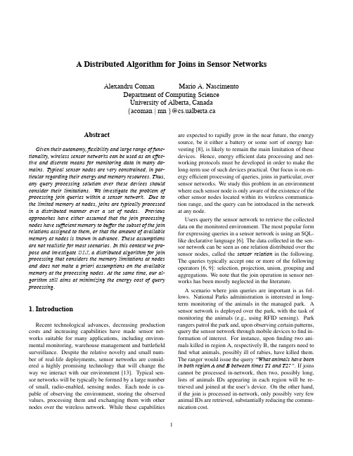
A Distributed Algorithm for Joins in Sensor NetworksAlexandru Coman Mario A.NascimentoDepartment of Computing ScienceUniversity of Alberta,Canada{acoman|mn}@cs.ualberta.caAbstractGiven their autonomy,flexibility and large range of func-tionality,wireless sensor networks can be used as an effec-tive and discrete means for monitoring data in many do-mains.Typical sensor nodes are very constrained,in par-ticular regarding their energy and memory resources.Thus, any query processing solution over these devices should consider their limitations.We investigate the problem of processing join queries within a sensor network.Due to the limited memory at nodes,joins are typically processed in a distributed manner over a set of nodes.Previous approaches have either assumed that the join processing nodes have sufficient memory to buffer the subset of the join relations assigned to them,or that the amount of available memory at nodes is known in advance.These assumptions are not realistic for most scenarios.In this context we pro-pose and investigate DIJ,a distributed algorithm for join processing that considers the memory limitations at nodes and does not make a priori assumptions on the available memory at the processing nodes.At the same time,our al-gorithm still aims at minimizing the energy cost of query processing.1.IntroductionRecent technological advances,decreasing production costs and increasing capabilities have made sensor net-works suitable for many applications,including environ-mental monitoring,warehouse management and battlefield surveillance.Despite the relative novelty and small num-ber of real-life deployments,sensor networks are consid-ered a highly promising technology that will change the way we interact with our environment[13].Typical sen-sor networks will be typically be formed by a large number of small,radio-enabled,sensing nodes.Each node is ca-pable of observing the environment,storing the observed values,processing them and exchanging them with other nodes over the wireless network.While these capabilitiesare expected to rapidly grow in the near future,the energy source,be it either a battery or some sort of energy har-vesting[8],is likely to remain the main limitation of these devices.Hence,energy efficient data processing and net-working protocols must be developed in order to make the long-term use of such devices practical.Our focus is on en-ergy efficient processing of queries,joins in particular,over sensor networks.We study this problem in an environment where each sensor node is only aware of the existence of the other sensor nodes located within its wireless communica-tion range,and the query can be introduced in the network at any node.Users query the sensor network to retrieve the collected data on the monitored environment.The most popular form for expressing queries in a sensor network is using an SQL-like declarative language[6].The data collected in the sen-sor network can be seen as one relation distributed over the sensor nodes,called the sensor relation in the following.The queries typically accept one or more of the following operators[6,9]:selection,projection,union,grouping and aggregations.We note that the join operation in sensor net-works has been mostly neglected in the literature.A scenario where join queries are important is as fol-lows.National Parks administration is interested in long-term monitoring of the animals in the managed park.A sensor network is deployed over the park,with the task of monitoring the animals(e.g.,using RFID sensing).Park rangers patrol the park and,upon observing certain patterns, query the sensor network through mobile devices tofind in-formation of interest.For instance,uponfinding two ani-mals killed in region A,respectively B,the rangers need to find what animals,possibly ill of rabies,have killed them.The ranger would issue the query“What animals have been in both region A and B between times T1and T2?”.If joins cannot be processed in-network,then two,possibly long, lists of animals IDs appearing in each region will be re-trieved and joined at the user’s device.On the other hand, if the join is processed in-network,only possibly very few animal IDs are retrieved,substantially reducing the commu-nication cost.1In this paper we focus on the processing of the join op-erator in sensor networks.Since the energy required for communication is three to four orders of magnitude higher than the energy required by sensing and computation[9], it is important to minimize the energy cost of communica-tion during query processing.Recently,a few works ad-dressed in-network processing of join queries.Bonfils and Bonnet[3]investigate placing a correlation operator at a node in the network.Pandit and Gupta[11]propose two algorithms for processing a range-join operator in the net-work and Yu at al.[16]propose an algorithm for processing equi-joins.These works study the self-join problem where subsets of the sensor relation are joined.Abadi et al.[1]pro-pose several solutions for the join with an external relation, where the sensor relation is joined with a relation stored at the user’s an et al.[5]study the cost of several join processing solutions with respect to the location of the network region where the join is performed.Most previous solutions either assume that nodes have sufficient memory to buffer the partition of the join relations assigned to them for processing,or that the amount of memory available at each node is known in advance and the assigned data par-titions can be set accordingly.These assumptions are un-realistic for most scenarios.It is well known that sensor networks are very constrained on main memory and the en-ergy cost of using theirflash storage(for those devices that have it)is rather prohibitive to be used for data buffering during query processing.In addition,in large scale sensor networks,it is not feasible for the sensor nodes or the user station to be aware of up-to-date information on memory availability of all network nodes.In this paper our contributions are three-fold.First we analyze the requirements of a distributed in-network join processing algorithm.Second,to our knowledge,this is the first work to develop and discuss in details a distributed al-gorithm for in-network join processing.Third,based on the present algorithm,we develop a cost model that can be used to select the most efficient join plan during the execution of the query.Our join algorithm is general in the sense that it can be used with different types of joins,including semi-joins,with minor modifications to the presented algorithm and cost model.As well,our algorithm can be used within the core of other previously proposed join solutions for re-laxing their assumptions on memory availability.2.BackgroundIn our work we consider a sensor network formed by thousands offixed nodes.Each node has several sensing units(e.g.,temperature,RFID reader),a processor,a few kilobytes of main memory for buffer and data processing,a few megabytes offlash storage for long-term storage of sen-sor observations,fixed-range wireless radio and it is battery operated.These characteristics encompass a wide range ofsensor node hardware,making our work independent of aparticular sensor platform.Further on,we consider thateach node is aware of its location,which is periodicallyrefreshed through GPS or a localization algorithm[14]toaccount for any variation in a node’s position due to envi-ronmental hazards.Each node is aware of the nodes locatedwithin its wireless range,which form its1-hop neighbour-hood.A node communicates with nodes other than its1-hop neighbours using multi-hop routing over the wirelessnetwork.As sensor nodes are not designed for user inter-action,users query the sensor network through personal de-vices,which introduce the query in the network through oneof the nodes in their vicinity.We consider a sensor network deployment where nodesacquire observations periodically and the observations arestored locally for future querying.The data stored at thesensor nodes forms a virtual relation over all nodes,denotedR∗.As nodes store the acquired data locally,each node holds the values of the observations recorded by its sensingunits and the time when each recording was performed.We analyze the self-join processing problem in sensornetworks,i.e.,the joined relations are spatially and tempo-rally constrained subsets of the sensor relation R∗.We im-pose no restrictions on the join condition,that is,any tuplefrom a relation could match any tuple of the other relation.For instance,the query“What animals have been in bothregions R A and R B between times T1and T2?”(from ourexample in Section1)can be expressed in pseudo-SQL as:SELECT S.animalIDFROM R∗as S,R∗as TWHERE S.location IN Region R AAND T.location IN Region R BAND S.time IN TimeRange[T1,T2]AND T.time IN TimeRange[T1,T2]AND S.animalID=T.animalIDLet us denote by A the subset of R∗restricted to Region R A and by B the subset of R∗restricted to Region R B. The query may also contain other operators ops(selection, projection,etc.)on each tuple of R∗or on the result of the join.As our focus is on join processing,we consider the relations A and B as the resulting relations after the query operators that can be applied individually on each node’s relation have been applied.We assume operators that can be processed locally by each sensor node on its stored relation and thus they do not involve any communication.We denote with J the result of the join of relations A and B,including any operators on the join result required by the query:J= ops J(A B).We assume operators on the join result can be processed in a pipelined fashion immediately following the join of two tuples.A general query tree and the notations we use are shown in Figure1.A UU opsJopsAopsopsAR iR jkR RmR oR nR pops BopsBopsBopsBJBAFigure1.Query tree and notations3.DIJ:A Distributed Join Processing Algo-rithm for Sensor NetworksJoin processing in sensor networks is a highly complex operation due to the distributed nature of the processing and the limited memory available at nodes.We discuss some of the requirements of an effective and efficient join pro-cessing algorithm for sensor networks,namely:distributed processing,memory management and synchronized com-munication.•Distributed processing.In large scale sensor net-works the join operation must be processed in a dis-tributed manner using localized knowledge.For most queries no single node can buffer all the data required for the join.In addition,no node(or user station) has global network knowledge tofind the optimal join strategy.As nodes have information only about their neighbourhood,the challenge is to take correct and consistent decisions among nodes with respect to pro-cessing the join.For instance,when the join operation is evaluated over a group of nodes,each node in the group must route and buffer tuples such that each pair of join tuples is evaluated exactly once in the join.•Memory management.Each node participating in the join must have sufficient memory to buffer the tu-ples that it joins and the resulting tuples.For some join queries the join relations are larger than the avail-able memory of a single node.Typically,several nodes must collaborate to process the join operator,pooling their memory and processing resources together.A join processing algorithm should pool these resources together and allocate tasks and data among the partici-pating nodes such that the efficiency of the processing is maximized.•Synchronized dataflow.Inter-node communication must be synchronized such that a node does not re-ceive new tuples to process when its memory is full.Otherwise,the node would have to drop some of the buffered or new tuples,which is unacceptable as it may invalidate the result of the join.Thus,each node mustfully process the join tuples it holds before receivingany new tuples.A similar problem occurs also for thenodes routing the data.A parent node routing data formultiple children may not be able to buffer all receiveddata before it can forward it.Thus,a join processingalgorithm should carefully consider theflow of dataduring its execution.In this work we propose a distributed join processing al-gorithm which considers the above requirements.In ourpresentation we focus on the join between two restrictions(A and B)of the R∗relation,where the join condition isgeneral(theta-join).Thus,every pair of tuples from re-lations A and B must be verified against the join condi-tion.Relations A and B are located within regions R A andR B and they are joined in-network in a join region R J. Technique forfinding the location of the join region havebeen presented elsewhere[4,5,16]and are orthogonal toour problem.In fact,our algorithm is general with respectto the join relations and their locations and could be usedwithin the core of other previously proposed join solutions(e.g.[5]),including solutions using semi-joins(e.g.[16]).For clarity of presentation we describe our join algorithm inthe context of the Mediated Join[5]solution.The Mediated Join solution works as follows:relationsA andB are sent to the join region(R J)where they are joined and the resulting relation J is transmitted to the query originator node.(Recall that a query can be posed at any node of the network.)Figure2shows in overview the query processing steps and the dataflow.The Mediated Join seems straightforward based on this description,but there are several issues that must be carefully addressed in the low-level sensor implementation to ensure the correct-ness of the query result,e.g.:•How to ensure that both relation A and B are transmit-ted to the same region R J?•How large should region R J be to have sufficient re-sources,i.e.,memory at nodes,to process the join?•How should A and B be transmitted such that the join is processed correctly at the nodes in R J?•How to process the join in R J such that the join is processed correctly using minimum resources?We now describe in details DIJ,our join processing al-gorithm addressing these questions.The steps of DIJ are: 1.Multi-cast the query from originator node O to nodesin R A and R B.Designate the nodes closest to the cen-tres C A and C B of the regions R A,respectively R B,as regional coordinators.Designate the coordinator lo-cation C J for join region R J.Disseminate the infor-mation about the coordinators along with the query.Figure2.Mediated Join-dataflow2.Construct routing trees in regions R A and R B rootedat their respective coordinators C A and C B.3.Collect information on the number of query relevanttuples for each region at the corresponding coordina-tors.Each coordinator sends this information to coor-dinator C J of the join region R J.4.Construct the join region.C J constructs R J so that ithas sufficient memory space at its nodes to buffer A.5.Distribute A over R J.(a)C J asks C A to start sending packets with tuples.Once C J receives A’s tuples,it forwards them toa node in R J with available memory.(b)Upon receiving a request for data from C J,C Aasks for relevant tuples from its children in therouting tree.The process is repeated by all inter-nal tree nodes until all relevant tuples have beenforwarded up in the tree.6.Broadcast B over R J(a)Once C J receives a signal from C A that it hasno more packets(i.e.,tuples)to send,C J asksfor one packet with tuples from C B.When thepacket is received,it is broadcast to nodes in R J.(b)Each node in R J joins the tuples in the packet re-ceived from B with its local partition of A,send-ing the resulting tuples to O.Once the join iscomplete,each node asks for another packet ofB’s tuples from C J.(c)Upon receiving a request for tuples from C J,C Basks for a number of join tuples from its childrenin the routing tree.The process is repeated byall internal tree nodes if they cannot satisfy therequest alone.(d)Once C J receives requests for B’s tuples from allnodes in R J,Step6is repeated unless C B signalsthat it has no more packets(i.e.,tuples)to send.In the steps above we chose,only for the sake of presen-tation,that relation A is distributed over the nodes in R J and relation B is broadcast over the nodes in R J.The steps above are symmetrical if the roles of A and B are switched, however the actual order does matter in terms of query cost. In Section4we explore this issue and show how to deter-mine which relation should be distributed and which should be broadcast in order to minimize the cost of the processing the join operator.Steps1-3of DIJ are typical to in-network query pro-cessing and do not present particular challenges.In Step4, the join coordinator C J must request and pool together the memory of other nodes in its vicinity for allocating relation A to these nodes(in Step5a).This is a non-trivial task as C J does not have information about the nodes in its vicin-ity(except its1-hop neighbours).Steps5and6also pose a challenge,that is,how to control theflow of tuples effi-ciently without buffer overflows,ensuring correct execution of the join.We detail these steps in the following.3.1.Constructing the join region(Step4)Once node C J receives the size of the join relations A and B from C A and C B(in Step1),it mustfind the nodes in its vicinity where to buffer relation A.DIJ uses the fol-lowing heuristic for this task,called k-hop-pooling: If C J alone does not have sufficient memory tobuffer relation A,C J asks its1-hop neighbours toreport how much memory they have available forprocessing the query.If relation A is smaller thanthe total memory available at the1-hop neigh-bours,C J stops the memory search.Otherwise,C J asks its2-hop neighbours to report their avail-able memory.This process is repeated for k-hops,where k represents the number of hops such thatthe total memory available at the nodes up to khops away from C J plus the memory available atC J is sufficient to buffer relation A.An interesting question is how much memory should a node allocate for processing a particular query.If the sensor network processes only one join query at a time(e.g.,there is a central point that controls the insertion of join queries in the network),then nodes can allocate all the memory they have available for processing the join.However,if nodes al-locate all their memory for a query,but several join queries are processed simultaneously in the network,it may happen that a coordinator C J will notfind any nodes with available memory in its immediate vicinity,forcing it to use farther away nodes during processing,and,thus,consuming more energy.For networks where multiple queries may coexist in the network,nodes should allocate only a part of their avail-able memory for a certain query,reserving the rest for other queries.How to actually best allocate the memory of an individual node is orthogonal to our problem.In this work we assume that nodes report as available only the memorythey are willing to use for processing the requested query.Figure3shows a possible memory allocation scheme at anode.3.2Distributing A over R J(Step5)In this step two tasks are carried out concurrently:C Arequests and gathers relevant tuples(grouped in data pack-ets)from R A,and C J distributes the packets received fromC A over R J.Once the set of k-hop neighbours that will buffer A hasbeen constructed,C J asks for relation A from C A,packetby packet,and distributes each packet of A’s tuples in around-robin fashion to its neighbours,ordered by their hopdistance to C J.When deciding to which node to send a newpacket with A’s tuples,a straightforward packet allocationstrategy would be for C J to pick a node from its list andsend to it all new packets with A’s tuples until its allocatedmemory is full.This strategy has two disadvantages.As allpackets use the same route(for most routing algorithms)toget to their destination node,their delivery will be delayed ifthere is a delay on one of the links in the route.Also,con-secutive packets may contain tuples with values such thatthey all(or many of them)will join with the same tuple inB.In this case,the node holding all these tuples will gener-ate many result tuples that have to be transmitted,delayingthe processing of the join.The hop-based round-robin al-location also ensures that all k-hop neighbours have a fairchance of having some free memory at the end of the allo-cation process,memory that can be used for other queries.Once node C A receives a request for tuples from C J,ithas to gather relevant tuples from R A.If C A would simplybroadcast the tuple request in the routing tree constructedover R A,nodes in R A will start sending these tuples to-ward C A.As each internal tree node has(likely)severalchildren,it should receive and buffer many packages beforebeing able to send these packages out.Some nodes maynot be able to handle such a dataflow due to lack of bufferspace,possibly dropping some of the packets.To ensurethat no packages are lost due to lack of buffer space,wepropose aflow synchronization scheme where each nodewill only buffer one package.In this scheme,the requestfor A’s tuples is transmitted one link at a time.Each nodein the routing tree is in one of the following states duringthe synchronized tupleflow(Figure4):•Wait for a tuple request from the parent node(or C J in the case of C A)in the routing tree constructed in Step2.•Send local tuples(from the local storage or receive buffer)to the parent node.•If buffer space has been freed and there are relevant tu-ples available at the children nodes in the routing tree,Figure3.Memory allocation schemeFigure4.A node’s states during tuple routingrequest tuples from a child node that still has tuples to send.Figure5shows the routing tree for a region and the information maintained in each node of the tree as tuples are routed from either R A or R B to R J.Note that the number of tuples that each child node will pro-vide has been collected as part of Step3.•Receive tuples from child,buffer the tuples and update the number of tuples that the child still has available.Once a node has forwarded to its parent all of A’s tuples from its routing sub-tree,it can free all buffers used for pro-cessing the query.{local: 2 tuples}{local: 2 tuples{local: 0 tuples}{local: 3 tuples}{local: 3 tuples}{local: 2 tuples{local: 3 tuplesN5: 8 tuplesN6: 5 tuples}N3: 0 tuplesN1: 2 tuplesN2: 3 tuples}N4: 3 tuples}N7N5N1N2N3N6N4Figure5.Join tuples information at nodes3.3.Broadcasting B over R J(Step6)The collection of B’s tuples proceeds much like the collection of A’s tuples,with one important difference. Whereas C A gathers and sends all of the relevant tuples of A as a a result of a single tuple request from C J,C B only sends one packet with tuples for each request it re-ceives from C J.This way,C J can broadcast such a packet of tuples to all nodes in R J,wait until all nodes fully pro-cess the local joins and send the results,and then request a new packet of tuples from R B when each node in the join region R J is ready to receive and join a new set of tuples.4.Selecting the relation to be distributedIn the previous discussions we have assumed for clarity of presentation that relation A is distributed over the nodes in region R J and B is broadcast over the nodes in the re-gion.An interesting question is which of the two join rela-tion should be distributed and whether the choice makes a major difference in cost.Let us focusfirst on which of the two join relation should be distributed and,subsequently,which should be incre-mentally broadcast.To decide on this matter,the query optimizer has to estimate the cost of the two options(i.e., distribute A or B)and compare their costs to decide which alternative is more energy efficient.For generality,we de-rive in the following a cost model for processing the join by distributing relation R d and broadcasting relation R b.The actual relations A and B can then be substituted into R d and R b(or vice-versa)to estimate the processing costs.Considering the steps of DIJ,the cost of query process-ing can be decomposed into a sum of components,with one component associated to each step.Several of these com-ponents are independent of the choice of the relation that is distributed.Thus,they do not affect the decision of which relation to distribute and do not need to be derived.For instance,we have the cost for disseminating the query in regions A and B(Step1)and the cost for constructing the routing tree over regions R A and R B(Step2).These costs are identical when processing the join by distributing A or B and do not affect the decision.The steps that have differ-ent costs when A or B are the distributed relation R d are the construction of the join region R J(Step4),the distribution of the relation R d(Step5a)and the broadcast of the relation R b(Step6a).Note that we are only interested in differences in the communication cost between the two alternatives. 4.1.Constructing the join region(Step4)As discussed in Section3.1,we use the k-hop-pooling strategy to construct the join region R J.In each round of memory allocation,C J broadcasts its request for memory in a hop-wise increasing fashion,until sufficient nodes with the required buffer space are located.During a round h,each node within h-hops from C J broadcast the memory request and its1-hop neighbours re-ceive the request message.Thus,the total energy cost is:E memreq4=k−1h=0(E t N h n M r+E r N h n N1n M r),where N h n represents the average number of nodes within h hops from a node,E t and E r represents the energy required to transmit,respectively receive,one bit of information and M r represents the size of the memory request message(in bits).N h n is a network-dependent value independent of our technique and it is derived in the Appendix.When a node receives a memory request message for the first time,it allocates buffer space in its memory and sends the memory information to C J.The nodes located h-hops away from C J perform two tasks:they send their own mem-ory information to the nodes located h−1hops away;and they forward the information they have received from the nodes located between h+1and k hops away from C J.If we denote by M i the size of the memory information for one node,the total energy cost of collecting the information on available memory is:E meminfo4=kh=1((E t+E r)(N h n−N h−1n)M i+(E t+E r)(N k n−N h n)M i)=(E t+E r)(kN k n−k−1h=1N h n)M iNote that(N h n−N h−1n)represents the number of nodesh-hops away and(N k n−N h−1n)represents the number of nodes located more than h and up to k hops away from C J. The total energy cost of the fourth step of DIJ is:E4=E memreq4+E meminfo4.Note that the costs of Step4do not depend on the join re-lations directly,but through k which determines the size of the join region R J and it is determined by the size of the join relation R d.Let B s be the average size(in bits)of the buffer space that each node in R J can allocate for processing the query. The minimum number of nodes that must be used to store relation R d in region R J is||R d||B s,where||R||denotes the size(in bits)of relation R.Since nodes are added to R J in groups based on their hop distance,k is the lowest number of hops such that the nodes within k hops from C J have sufficient buffer space to buffer R d:k={min h|N h n B s≥||R d||}.。
Oracle Argus Safety 8.1 用户指南说明书

U.S. GOVERNMENT END USERS: Oracle programs, including any operating system, integrated software, any programs installed on the hardware, and/or documentation, delivered to U.S. Government end users are "commercial computer software" pursuant to the applicable Federal Acquisition Regulation and agency-specific supplemental regulations. As such, use, duplication, disclosure, modification, and adaptation of the programs, including any operating system, integrated software, any programs installed on the hardware, and/or documentation, shall be subject to license terms and license restrictions applicable to the programs. No other rights are granted to the U.S. Government.
第4章贪心算法-1解读

时间复杂性 排序:O(n log n) 其它:O(n) 为什么采用贪心策略能得到最优解?
2018年11月19日星期一
第4章 贪心算法
11
0 / 1背包问题的几种贪婪策略: 1)从剩余的物品中,选出可以装入背包的价值最大的 物品 2)从剩下的物品中选择可装入背包的重量最小的物品 3)从剩余物品中选择可装入包的pi /wi 值最大的物品 这三种策略都不能保证得到最优解。 我们不必因所考察的几个贪婪算法都不能保证得到 最优解而沮丧, 0 / 1背包问题是一个NP复杂问题。 对于这类问题,也许根本就不可能找到具有多项式 时间的算法。
(1/2, 1/3,1/4) (1,2/15,0) (0,2/3,1) (0,1,1/2)
选取度量标准是用贪心法求解问题的关键。
2018年11月19日星期一
第4章 贪心算法
10
用贪心算法求解背包问题的步骤: 1)计算每种物品的单价vi/wi 2)按物品的单价,从大到小排序 3)单价高的物品优先装包,直至装满。 (最后一种物品可能装入一部分)
2018年11月19日星期一
第4章 贪心算法
3
Байду номын сангаас
贪心算法常常用于求解某些问题的最优解。 这类问题一般有n个输入,而其解由这n个输入的 某个子集组成,要求该子集满足预先给定的约束 条件。这一子集称为该问题的一个可行解。其中 使目标函数取得极值的可行解称为最优解。
约束条件 可行解 准则 最优解
N个输入
2018年11月19日星期一
第4章 贪心算法
12
虽然按pi /wi 非递增的次序装入物品不能保证得到 最优解,但它是一个直觉上近似的解。我们希望 它是一个好的启发式算法,且大多数时候能很好 地接近最后算法。 据统计,在600个随机产生的背包问题中,用这种 启发式贪婪算法来解有 239 题为最优解。有 583 个 例子与最优解相差10%,所有600个答案与最优解 之差全在 25% 以内。该算法能在 O(n log n) 时间内 获得如此好的性能。我们也许会问,是否存在一 个x (x<100 ),使得贪婪启发法的结果与最优值相 差在x%以内。答案是否定的。
放学几点写作业英语

When it comes to doing homework after school,the timing can vary greatly depending on individual schedules,school hours,and personal preferences.Here are some general guidelines and tips for managing homework effectively:1.Immediate After School:Some students find it helpful to start their homework as soon as they get home from school.This can be a good strategy if youre still fresh and can focus well immediately after a day of learning.2.After a Break:If you feel drained after school,it might be beneficial to take a short break before starting your homework.A break could involve a snack,a short walk,or a relaxation activity to recharge.3.Dedicated Homework Time:Establish a routine by setting aside a specific time each day for homework.This could be right after school,after dinner,or before bedtime, depending on what works best for you.4.Prioritize Tasks:If you have multiple assignments,prioritize them based on due dates and difficulty.Tackle the most challenging or timeconsuming tasks first when your energy levels are highest.5.Break It Down:Large assignments can be overwhelming.Break them down into smaller,manageable tasks and tackle them one at a time.6.Create a Study Environment:Find a quiet,comfortable place to do your homework where you can focus without distractions.e a Planner or Calendar:Keep track of assignments and due dates using a planner or digital calendar.This can help you stay organized and manage your time effectively.8.Avoid Procrastination:Its easy to put off homework,but this can lead to stress and poor performance.Try to start your work as soon as possible to avoid lastminute rushes.9.Ask for Help:If youre struggling with a particular subject or assignment,dont hesitate to ask your teacher,a tutor,or a classmate for help.10.Take Regular Breaks:Studies show that taking short breaks can improve focus and e techniques like the Pomodoro Technique,where you work for25 minutes and then take a5minute break.11.Stay Healthy:Make sure youre getting enough sleep,eating well,and exercisingregularly.These factors can greatly affect your ability to concentrate and complete homework efficiently.12.Reflect on Your Progress:At the end of each week,take some time to review what youve accomplished and what you can improve on for the next week.Remember,the best time to do homework is when you can focus and be productive.Its important to find a routine that fits your lifestyle and helps you manage your schoolwork effectively.。
an efficient approach to clustering large multimedia databases with noise
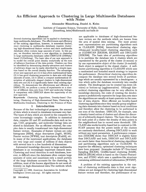
Abstract Several clustering algorithmscan be applied to clustering in large multimediadatabases. The effectiveness and efficiency of the existing algorithms, however, is somewhat limited, since clustering in multimediadatabases requires clustering high-dimensional feature vectors and since multimedia databases often contain large amountsof noise. In this paper, we therefore introduce a new algorithm to clustering in large multimedia databases called DENCLUE (DENsitybased CLUstEring). The basic idea of our new approach is to modelthe overall point density analytically as the sum of influence functions of the data points. Clusters can then be identified by determiningdensity-attractors and clusters of arbitrary shape can be easily described by a simple equation based on the overall density function. The advantages of our newapproachare (1) it has a firm mathematical basis, (2) it has goodclustering properties in data sets with large amountsof noise, (3) it allows a compactmathematicaldescription of arbitrarily shapedclusters in high-dimensional data sets and(4) it is significantly faster than existing algorithms. To demonstratethe effectiveness and efficiency of DENCLUE, perform a series of experiments on a numwe ber of different data sets from CAD molecular biology. and A comparison with DBSCAN shows the superiority of our new approach. Keywords: Clustering Algorithms, Density-based Clustering, Clustering of High-dimensional Data, Clustering in MultimediaDatabases, Clustering in the Presence of Noise 1 Introduction Because of the fast technological progress, the amount of data which is stored in databases increases very fast. The types of data which are stored in the computer become increasingly complex. In addition to numerical data, complex 2D and 3D multimedia data such as image, CAD,geographic, and molecular biology data are stored in databases. For an efficient retrieval, the complex data is usually transformed into high-dimensional feature vectors. Examples of feature vectors are color histograms [SH94], shape descriptors [Jaggl, MG95], Fourier vectors [WW80], text descriptors [Kuk92], etc. In many of the mentioned applications, the databases are very large and consist of millions of data objects with several tens to a few hundreds of dimensions. Automated knowledge discovery in large multimedia databases is an increasingly important research issue. Clustering and trend detection in such databases, however, is difficult since the databases often contain large amounts of noise and sometimes only a small portion of the large databases accounts for the clustering. In addition, most of the knownalgorithms do not work efficiently on high-dimensional data.The methods which Copyright(c) 1998, American Association for Artificial Intelligence (). rights reserved. All 58 Hinneburg
k-center-greedy原理
k-center-greedy原理
K-Center-Greedy是一种常见的贪心算法,用于解决K-Center
问题。
K-Center问题是指在给定一组点和一个整数K的情况下,找
到K个点作为中心,使得这K个点到其他所有点的最大距离最小。
K-Center-Greedy算法的基本原理如下:
1. 初始化:选择一个点作为初始中心点,并将其加入中心点集
合C。
2. 迭代:重复以下步骤直到找到K个中心点:
a. 对于每个非中心点P,计算P到C中所有点的最小距离,选择最大的距离作为当前点P到中心点集合C的距离。
b. 选择距离最大的点作为新的中心点,并将其加入中心点
集合C。
3. 输出:返回中心点集合C作为解。
K-Center-Greedy算法的核心思想是通过贪心的方式逐步选择
距离最远的点作为中心点,以使得选择的中心点集合能够覆盖到其
他所有点,并且最大距离最小。
K-Center-Greedy算法的时间复杂度是O(K(N-K)N),其中N是
点的总数。
这是因为在每次迭代中,需要计算每个非中心点到中心
点集合的距离,共需计算(K(N-K))次。
同时,还需要选择距离最大
的点作为新的中心点,这需要遍历所有非中心点,共需遍历N次。
K-Center-Greedy算法的优点是简单易实现,并且在许多实际
问题中表现良好。
然而,该算法可能不一定能够找到全局最优解,
因为它是基于局部最优选择的贪心算法。
为了得到更好的解,可以
尝试使用其他启发式算法或者精确算法来解决K-Center问题。
背包问题的目标函数和贪心算法最优化量度标准
背包问题的目标函数和贪心算法最优化量度标准
贪心算法是一种较为简单的解决给定问题的优化方法,其具有从利益最优点出发搜索解决方案,实现最优化的优点。
常用在求解最大化或最小化某固定目标函数的问题上。
利用贪心算法可以轻松求解背包问题。
背包问题是指在满足总重量不超过某一给定值的条件下,背包问题最多能容纳多少物体,以及如何选择这些物体,使满足给定总重量的情况下的总价值最大化。
背包问题的目标函数一般可以设计成最大化总价值函数和最大化总重量函数。
在背包问题中,贪心算法最优化量度标准一般是以价值/重量比作为最佳选择标准,从而让计算机可以快速地预测出价值/重量比最大的物品,以达到最优化的效果。
贪心算法的最优化量度标准的例子是在背包问题中,我们可以把所有物品按其价值/重量比从大到小排列,然后依次将相应的物品装入背包,直至背包满或剩余的物品的价值/重量比不高于已经放入背包中的物品的价值/重量比。
因此,贪心算法在背包问题中的优化量度标准一般是以价值/重量比作为最佳选择标准,从而让计算机可以快速地预测并实现最优化的效果。
而该目标函数则是在满足总重量不超过某一给定值的条件下,最多能容纳多少物体,以及如何选择这些物体,使满足给定总重量的情况下的总价值最大化。
Spark经典论文笔记---ResilientDistributedDatasets:AF。。。
Spark经典论⽂笔记---ResilientDistributedDatasets:AF。
Spark 经典论⽂笔记Resilient Distributed Datasets : A Fault-Tolerant Abstraction for In-Memory Cluster Computing为什么要设计spark现在的计算框架如Map/Reduce在⼤数据分析中被⼴泛采⽤,为什么还要设计新的spark?Map/Reduce提供了⾼级接⼝可以⽅便快捷的调取计算资源,但是缺少对分布式内存有影响的抽象。
这就造成了计算过程中需要在机器间使⽤中间数据,那么只能依靠中间存储来保存中间结果,然后再读取中间结果,造成了时延与IO性能的降低。
虽然有些框架针对数据重⽤提出了相应的解决办法,⽐如Pregel针对迭代图运算设计出将中间结果保存在内存中,HaLoop提供了迭代Map/Reduce的接⼝,但是这些都是针对特定的功能设计的不具备通⽤性。
针对以上问题,Spark提出了⼀种新的数据抽象模式称为RDD(弹性分布式数据集),RDD是容错的并⾏的数据结构,并且可以让⽤户显式的将数据保存在内存中,并且可以控制他们的分区来优化数据替代以及提供了⼀系列⾼级的操作接⼝。
RDD数据结构的容错机制设计RDD的主要挑战在与如何设计⾼效的容错机制。
现有的集群的内存的抽象都在可变状态(啥是可变状态)提供了⼀种细粒度(fine-grained)更新。
在这种接⼝条件下,容错的唯⼀⽅法就是在不同的机器间复制内存,或者使⽤log⽇志记录更新,但是这两种⽅法对于数据密集(data-intensive⼤数据)来说都太昂贵了,因为数据的复制及时传输需要⼤量的带宽,同时还带来了存储的⼤量开销。
与上⾯的系统不同,RDD提供了⼀种粗粒度(coarse-grained)的变换(⽐如说map,filter,join),这些变换对数据项应⽤相同的操作。
greedysoup策略
greedysoup策略在计算机科学中,贪心算法(greedy algorithm)是一种通过每一步都选择当前最优解的策略来求解问题的方法。
与动态规划算法相比,贪心算法通常更加简单高效,但也存在一些问题不能通过贪心算法来解决。
贪心算法的基本思想是,每一步都选择当前最优解,不考虑对后续步骤的影响。
这种局部最优解的选择方式可以保证整体的最优解,从而达到求解问题的目的。
贪心算法通常适用于满足“最优子结构”和“贪心选择性质”的问题。
最优子结构是指问题的最优解可以通过子问题的最优解来构造。
贪心选择性质是指每一步都选择当前最优解,并且这个选择不依赖于后续步骤的选择。
这两个性质是贪心算法能够成功求解问题的关键。
贪心算法的应用非常广泛,常见的问题包括最小生成树、单源最短路径、背包问题等。
下面将通过几个例子来说明贪心算法的应用。
1. 最小生成树问题最小生成树问题是指在一个带权无向图中找到一棵包含所有顶点的生成树,使得树的权值之和最小。
贪心算法可以通过每次选择权值最小的边来构建最小生成树。
2. 单源最短路径问题单源最短路径问题是指在一个带权有向图中,求解从一个顶点到其他所有顶点的最短路径。
贪心算法可以通过每次选择当前距离最短的顶点来更新其他顶点的距离。
3. 背包问题背包问题是指给定一个固定大小的背包和一组物品,每个物品有自己的价值和重量,在背包中放入物品使得总价值最大。
贪心算法可以通过每次选择单位价值最高的物品来求解。
虽然贪心算法具有简单高效的特点,但并不是所有问题都适合使用贪心算法来求解。
贪心算法的局限性在于,它无法回退,一旦做出选择就无法撤销。
因此,在某些情况下,贪心算法求得的结果可能并不是全局最优解。
贪心算法是一种常用的求解问题的方法,通过每一步都选择当前最优解的策略,可以高效地求解一些问题。
然而,贪心算法并不适用于所有问题,需要根据具体情况进行选择。
在实际应用中,我们可以结合其他算法来进一步优化贪心算法的效果,以满足实际需求。
- 1、下载文档前请自行甄别文档内容的完整性,平台不提供额外的编辑、内容补充、找答案等附加服务。
- 2、"仅部分预览"的文档,不可在线预览部分如存在完整性等问题,可反馈申请退款(可完整预览的文档不适用该条件!)。
- 3、如文档侵犯您的权益,请联系客服反馈,我们会尽快为您处理(人工客服工作时间:9:00-18:30)。
A Greedy Distributed Time Synchronization Algorithm for Wireless Sensor Networks King-Yip Cheng,King-Shan Lui,Yik-Chung Wu and Vincent TamDepartment of Electrical and Electronic EngineeringThe University of Hong KongPokfulam Road,Hong Kong,ChinaAbstract—In this paper,a distributed network-wise synchro-nization protocol is presented.The protocol employs Pairwise Broadcast Synchronization(PBS)in which sensors can be syn-chronized by merely overhearing the exchange of synchronization packets.We investigate how to minimize the number of PBS required to synchronize all nodes in a network.We show that the problem offinding the minimum number of PBS required is NP-complete.A distributed greedy algorithm is proposed. The protocol is tested by extensive simulations.Although the algorithm behind is heuristic-based,the performance is closed to the centralized algorithm.The message overhead is compared with that of Timing-Sync Protocol for Sensor Networks(TPSN).I.I NTRODUCTIONIn recent years,wireless sensor networks(WSNs)have drawn much attention from the academia and industry as they offer an unprecedented range of potential applications[1][2]. Despite the wide scope of applications,resource-constrained WSNs introduce a lot of challenges for researchers to tackle. Performing time synchronization efficiently in WSN is one of the challenging tasks[3].In WSN applications involving data fusion,target tracking or event monitoring,precise timing information is critical to the functionality of the networks. Whenever an event is detected,packets will be sent to a data sink to report the event with two contexts,time and location of the event.Without coupling these two contexts,the detection of an event is meaningless to many applications.Time synchronization has been studied for a long time in wired distributed systems,but traditional time synchro-nization protocols are not suitable for resource-constrained WSNs.Therefore,many new time synchronization protocols are designed for WSNs.Most protocols are based on two fun-damental approaches,Sender-Receiver Synchronization(SRS) and Receiver-Receiver synchronization(RRS).The two ap-proaches differ by how the timing packets are exchanged between the synchronized node and the unsynchronized node. Although they enable pairwise synchronization in WSNs, extending pairwise time synchronization to network-wise time synchronization in an energy efficient manner is still an issue. Recently,Noh et al.[4]proposed a protocol for synchro-nization in WSNs called Pairwise Broadcast Synchronization (PBS)protocol which can greatly reduce the number of mes-sages required.Through overhearing synchronization packet exchanges,neighbouring nodes can synchronize themselves to the reference node.However,it requires two super nodes to broadcast the synchronization packets to the sensors.There is a lack of efficient distributed protocol to perform network-wise synchronization.In view of this,we propose a distributed multi-hop syn-chronization protocol with PBS in this paper.The protocol is designed for networks whose topologies remain static in a considerable period of time.The paper is organized as follows. Related works are discussed in Section II.Fundamental ap-proaches and existing protocols for synchronization in WSNs will be discussed.In Section III,we analyze the network-wise synchronization problem with PBS.We demonstrate that finding the minimum number of PBS operation for network-wise synchronization is an NP-complete problem.In Section IV,a distributed PBS-based network-wise synchronization protocol will be presented.The proposed protocol is justified by extensive simulations.Results are presented in Section V. The paper is concluded in Section VI.II.R ELATED W ORKSElson et al.[5]proposed a receiver-receiver protocol called Reference Broadcast Synchronization(RBS).A beacon node broadcasts beacons to a pair of receivers.The receiver marks the reception time and exchange the timestamps upon re-ceiving the beacons.Assuming that the propagation delay is negligible and there is no clock skew,the time offset between the receivers is the difference of the timestamps.Despite the simple procedures,providing periodic reference pulses is much more costly,especially in multihop manner.Special nodes are required to transmit the reference pulses or sensors take turns to broadcast the reference pulses periodically.However,both methods do not scale to large sensor networks.Maroti et al.[6]proposed a similar approach called Flood-ing Time Synchronization Protocol(FTSP).The sender broad-casts beacons with MAC-layer timestamps.Receivers do not need to exchange their timestamps of reception to estimate the clock offset.Clock skew can also be estimated using linear regression like RBS.However,the multihop synchronization protocol does not take energy efficiency into consideration. The timing information is distributed byflooding synchroniza-tion packets across the network.Ganeriwal et al.[7]proposed the Timing-sync Protocol for Sensor Network(TPSN).The protocol follows the sender-receiver approach.Nodes are synchronized in a pairwise manner.Timestamps are marked when packets are sent and received at both ends.After exchanging two packets,theFig.1.Synchronization sequence:(1→4),(1→7)sender obtains four timestamps,the sending and reception times of the packets.The clock offset between the sender and the receiver can be estimated by these timestamps.To extend the pairwise synchronization to multi-hop synchronization,a level discovery phase is placed before synchronizations are performed.The level discovery phase constructs a hierarchical structure in the network.Nodes are synchronized along the hierarchical structure starting from the root node.Sensors are synchronized by counterparts of the level that is immediately above.Sichitiu et al.[8]proposed two sender-receiver synchroniza-tion protocols called Tiny-Sync and Mini-Sync.Timestamps are exchanged and are used to establish bounds on the relative clock skew and offset.Tiny-Sync differs from Mini-Sync in terms of the storage and computational requirements.Noh et al.[4]proposed a receiver-only synchronization approach called Pairwise Broadcast Synchronization(PBS). PBS use the broadcast channel to synchronize nodes within a broadcast domain.Two super nodes,A,P,exchange timing information like TPSN.When the messages are overheard by node B,node B marks the arrival times and obtain the times-tamps broadcasted by node A and P.With these timestamps, sensor B can synchronize to node P.This greatly reduce the number of total message required for synchronizing nodes within a broadcast domain.Although PBS enables groupwise synchronization,there is no multihop synchronization protocol to extend PBS for network-wise synchronization.III.A NALYSIS OF N ETWORK-WISE S YNCHRONIZATIONWITH PBSIt is almost impossible to install two super nodes with communication ranges covering the whole sensor network.A multi-hop time synchronization protocol is needed for network-wise synchronization.To allow full play to the group-wise synchronization properties of PBS and reduce the number of PBS message exchange,the pairs performing PBS message exchange have to be chosen carefully.Figure1illustrates an example.Node1is the reference node.The rest of the nodes are unsynchronized and are neighbours of node 1. The number of PBS message exchange can be reduced by synchronizing with the node that the maximum number of unsynchronized nodes can be simultaneously synchronized by overhearing.Thus,a PBS message exchange is performed with node4.Node2to node6are synchronized at the same timeby overhearing.Node7is then synchronized by performinganother PBS message exchange with node1.In fact,node7can be synchronized by node6after node6is synchronized,but synchronizing with node1is more preferable as synchro-nization error will be accumulated.Although a solution can befound in this way,it may not be the best in terms of the numberof PBS performed.The problem becomes more complicatedwhen unsynchronized nodes are more than one-hop away fromthe reference node.These nodes can be synchronized by morethan one synchronized nodes.Suppose there are(N−1)unsynchronized nodes and onereference node.The network can be considered as a graph G(V,E).(v i,v j)∈E if node i and node j can communicate with each other.Levels representing the hop counts fromthe reference node are assigned to nodes.To minimize thesynchronization error,level(i+1)nodes should only besynchronized by nodes of level i,either through messageexchange or overhearing.Then the network-wise synchroniza-tion can be broken down into a number of independent sub-problems.Each sub-problem is to synchronize nodes of level (i+1)to nodes of level i by the least number of PBS message exchanges.In most scenarios,sub-problems are basically the same except for the sub-problem of synchronizing level1 nodes since there is only one reference node in level0.A.Synchronizing nodes of level1Let G(V,E)be a graph that V={v r,v1,...,v n}represents the set of nodes of level1and the reference node,v r.Let D be the synchronization set which is a subset of level1nodes. The reference node performs PBS with every node in D.We aim tofind a D such that for all nodes v i,i=r,at least one of the following conditions is met:•v i∈D such that v i can be synchronized by exchanging timing information with the reference node.•(v i,v j)∈E,for some v j∈D such that v i can be synchronized by overhearing the synchronization packets exchanged between v j and the reference node.This problem is NP-complete since it is NP-hard and we canreduce an instance of the dominating set problem to this Level1problem.An instance of dominating set problem consists ofa graph,G (V ,E )which V is the set of vertices and E is the set of edges.A dominating set K,is a subset of V such that for all(v i,v j)∈E ,either v i or v j or both are in K. It is NP-complete infinding the dominating set K with the minimum size.Given a dominating set instance G (V ,E ), we can reduce it to Level1problem,G(V,E),byV=V ∪{v r}E=E ∪{(v r,v i)|v i∈V }The reduction is illustrated in Figure2.Suppose that G has asynchronization set D⊆(V−{v r}),then for all non-reference node v i in(V−D),there exists a v j in D such that(v i,v j)∈E.Since v i,v j=v r,(v i,v j)∈E ,hence,D is the dominating set of G (V ,E ).'(',')G V E '{}'{(,)|'}r r i i V V v E E v v v V =∪=∪∈Fig.2.Reducing a dominating set problem to a Level 1problemB.Synchronizing nodes of level (i +1),i >0For i >0,it is very likely that any level (i +1)node can be synchronized by more than one node in level i ,for i >0.In this section,we analyze this sub-problem and we call this problem Higher Level Problem (HLP).Let G (V,E )be the graph representing the topology of level i nodes and level (i +1)nodes.V =V M V N is the set of vertices where V M ={m 1,...,m M }are nodes of level i and V N ={n 1,...,n N }are the nodes of level (i +1).Each edge,(j,k )∈E ,implies that connectivity exists between sensor j and sensor k .There are three types of edges in E :edges connecting nodes in V M only,edges connecting nodes in V N only,and edges connecting one node in V M and one node in V N .Note that every node in V N must be a neighbour of a node in V M .PBS messages can only be exchanged between a node in V M and a node in V N .When PBS is performed between m j and n k ,where m j ∈V M ,n k ∈V N and (m j ,n k )∈E,n k becomes synchronized and those nodes that are connected to both m j and n k can overhear the messages and get synchronized as well.Our HLP is to identify the smallest subset,D ,of E ,such that for every n l ∈V N ,at least one of the following conditions is met,•∃m j ∈V M s.t.(m j ,n l )∈D•∃(m j ,n k )∈D s.t.(m j ,n l ),(n k ,n l )∈E ,m j ∈V M ,n k ∈V N .Furthermore,we denote S j,k as the set of nodes that can be synchronized by performing PBS between node m j and node n k .It can be shown that the well-known NP-complete set covering problem [9]can be reduced to our HLP.A set covering problem instance (X,F )consists of a universe X and a family of subset F .Each element of X belongs to at least one subset m ,i.e.X =m ∈Fm The set covering problem is to find a subset of F of minimum size that covers all the elements of X .Given a set covering problem instance (X,F )which X ={n 1,...,n |X |}is the universe,and F :{m 1,m 2,...,m |F |}is a family of subsets,we map each n k to a node of level (i +1).We also map each subset m j to a level i node.Hence,V M ={m 1,...,m |F |}and V N ={n 1,...,n |X |}.For each m ∈F ,we include (n,m )in E for every n in subset m .Let n be the first element of a subset m ,we put (n ,n )in E for every n in the subset m .Then an instance of the sub-problem ism 22, m 3, m 4} 9}Fig.3.A set covering problem instance,(X,F )4} Fig.4.Sub-problem corresponding to set covering problem of Figure 3obtained.Figure 3is the original set covering problem andFigure 4is the corresponding HLP.We argue that A ⊆F is the family of subsets that covers all elements in the set covering problem iff D ={(a,n )|n is the first element in a,a ∈A }is a solution of HLP.If A is a set cover of V N ,performing PBS between (a,n )where n is the first element in a will synchronize all nodes in A .If PBS message exchanges are performed for all a in A ,then all nodes in V N will be synchronized as a covers all nodes in V N .Thus,D is a solution of HLP.If D ={(a,n )|n is the first element in a,a ∈A }is a solution of HLP,a subset of nodes in V N is associated to each a which is the subset of nodes that are synchronized by performing PBS message exchange between a and n .The family of subset of nodes that are associated to A must cover V N since every node in V N is synchronized by D .IV.A DISTRIBUTED G REEDY GLOBAL SYNCHRONIZATIONS PROTOCOL FOR WSN SIn the previous section,we have shown that the problem of finding the optimal synchronization set is of NP-complete.Although sub-optimal solutions for dominating set problems and set covering problems can be obtained by approximation algorithms [10], e.g.greedy algorithm,it is centralized in nature.Huge communication overheads will be incurred if the centralized greedy algorithm is applied in different levels.The overheads may overshadow the energy saved by using PBS.In view of this,we propose a distributed heuristic-based protocol for network-wise synchronization with PBS.Assumethat every node in the network has a unique ID and levels are assigned to sensors as in the level discovery phase presented in [7].The protocol for level i and level (i +1)nodes can be broken down into the following steps:(1)Nodes first discover how many neighbours they have.Neighbour information can be obtained when the level discovery phased is performed.A list,L j ,is created by each sensor j of level i .The list contains the IDs of all of its neighbours from level i .Every sensor of level i sends the list to its level (i −1)neighbours to notify them which level i sensors are their neighbours.Meanwhile,they also receive neighbour lists from nodes of level (i +1).(2)After receiving all neighbour lists from its level (i +1)neighbours,j can determine the maximum number of its neighbours that can be synchronized by one PBS.Let that number be sync num of j and that particular level (i +1)node be k (see Figure 5).The sync num of j will be sent to all level i neighbours of j .(3)Each level i node will receive all the sync num of its level i neighbours eventually.If the sync num of j itself is the largest among the received sync num ,j will send each level i neighbour a list,L ,which contains the IDs of the sensors that can be synchronized by performing a PBS message exchange with node k of level i +1.The ID of node k is stored in another list,the synchronization list.List L j of j is updated as L j =L j −L ,i.e.the synchronized nodes will be removed from the neighbour list of j .Hence,sync num is also updated and it must be smaller than the old value.The updated sync num of j is distributed together with L .If the updated sync num equals 0,j can jump to step (5),afterwards.Neighbours receiving the updated sync num of value 0are indirectly notified that they do not need to wait for any update from j anymore.If j finds that its sync num is not the maximum,it will send a packet not MAX to its level i neigbhours (see Figure 6).Then,j waits for replies from its neighbours and there are two possible scenarios for j after receiving all replies from its level i neighbours.•j receives one or more lists L and corresponding sync num from its level i neighbour(s)and packets not MAX from the rest of its level i neighbours.List L j will be updated as L j =L j −(L ).A new sync num can be determined.The new sync num will be distributed to all level i neighbours of j .If the updated sync num equals 0,j will jump to step (5)after sending the sync num .As mentioned before,neighbours of j will not wait for any update from it.•j receives packets not MAX from all of its level i neighbours.The sync num of j remains unchanged.Then,j will send its sync num to all of its level i neighbours again.This scenario is possible.The node which j thought to have the maximum sync num may not find itself have the maximum sync num .Thati+1)i-1)k Fig.5.Nodes exchanging neighbour lists and determining sync num(a)Nodes exchanging sync num with their neigbhours(b)Node with local maximum of sync num ,i.e.node 1,distributes list LFig.6.Local information exchangenode and j have two different neighbour sets.(4)Step (3)will be reiterated until L j becomes an empty list.(5)j starts performing PBS with the nodes in its synchro-nization list.All level (i +1)sensors must be synchronized eventually as there exist at least one sensor which finds itself having the maximum sync num after step (3)is iterated once by each level i sensor.V.S IMULATIONSimulations are conducted to justify our protocol.We do not focus on the timing accuracy since PBS is shown to be as accurate as RBS in [4].Instead,we study how many rounds of PBS message exchanges are required to achieve network-wise synchronization and the message overheads incurred by the heuristic algorithm.In the simulations,sensors are uniformlyFig.7.Averagenumber of PBS required for network-wise synchronization Fig.8.Average number of messages transmitted to achieve network-wisesynchronizationdistributed in a square munication ranges are equal among all sensors and are adjusted to give different degrees of connectivity,i.e.the average number of neighbours per node. 60network topologies are randomly generated for each setting.A.Number of PBS for Network-wise Synchronization Figure7gives the average number of PBS required to achieve network-wise synchronization with different degrees of connectivity using our proposed protocol.We compare the result with that obtained by the centralized greedy algorithm. The proposed protocol achieve performance close to that of the centralized works with200nodes and connectivity around7can be synchronized after around80 PBS are performed.If TPSN is used to synchronize the same200-node network,each node except the root node must synchronize with another node,giving199pairwise synchronizations.Therefore,the proposed protocol is more efficient than TPSN in terms of the number of pairwise synchronizations.B.Number of messages for Network-wise Synchronization Figure8presents the message overheads introduced by the proposed algorithm.The protocol is scalable with network size as information is only exchanged between immediate neigh-bours.More importantly,it is also scalable with network den-sities that most wireless sensor networks possess.The number of messages required grows modestly as the average number of neighbours increase.Even though increasing connectivity makes sensors have more neighbours to communicate with,it also reduces the number of PBS required to synchronize the whole network.Noted that the message overheads are one-off as long as the topology of the network does not change, but energy can be saved from each round of resynchronization. Using the results obtained from Figure7and Figure8,we can estimate how many rounds of resynchronizations will offset the one-off overheads.For400-node networks with average connectivity of8.13,the average number of PBS for network-wise synchronization is144.83and the overheads from our algorithm are1467.8messages.If the same networks are synchronized by TPSN,399pairwise synchronizations are re-quired.Since each PBS and TPSN synchronization require two message exchanges,after about3rounds of synchronization, the overheads from the proposed algorithm are cancelled out. In other words,after the third round of synchronizations,less energy is spent in resynchronization compared to TPSN.From the simulation results,the one-off overhead of the proposed algorithm is offset after3rounds of resynchronizations in all the topologies tested,when compared to TPSN.VI.C ONCLUSIONIn this paper,we propose a distributed protocol for multi-hop time synchronization in wireless sensor networks using Pairwise Broadcast Synchronization(PBS).We justify our heuristic-based proposal by showing thatfinding the optimal synchronization set is NP-complete.The performance of the protocol is examined by extensive simulations.Results show that the protocol is scalable with network size and connectivity. In the future,the protocol will be tested in real sensor networks.R EFERENCES[1] D.Estrin,indan,J.Heidemann,and S.Kumar,“Next centurychallenges:scalable coordination in sensor networks,”in Proc.of the 5th MobiCom,1999,pp.263–270.[2]I.F.Akyildiz,W.Su,and Y.Sankarasubramaniam,“Wireless sensornetworks:a survey,”Computer Networks,vol.38,pp.393–422,Mar.2002.[3]J.Elson and K.R¨o mer,“Wireless sensor networks:a new regime for timesynchronization,”SIGCOMM mun.Rev.,vol.33,no.1,pp.149–154,2003.[4]K.-L.Noh and E.Serpedin,“Pairwise broadcast clock synchronizationfor wireless sensor networks,”in IEEE International Workshop:From Theory to Practice in Wireless Snsor Networks(T2PWSN07),2007.[5]J.Elson,L.Girod,and D.Estrin,“Fine-grained network time synchro-nization using reference broadcasts,”SIGOPS Oper.Syst.Rev.,vol.36, no.SI,pp.147–163,2002.[6]M.Mar´o ti,B.Kusy,G.Simon,and´Akos L´e deczi,“Theflooding timesynchronization protocol,”in Proc.of the2nd SenSys,2004,pp.39–49.[7]S.Ganeriwal,R.Kumar,and M.B.Srivastava,“Timing-sync protocolfor sensor networks,”in Proc.of the1st ACM SenSys,2003,pp.138–149.[8]M.L.Sichitiu and C.Veerarittiphan,“Simple,accurate time synchro-nization for wireless sensor networks,”in Proc.IEEE WCNC,Mar.2003, pp.1226–1273.[9]R.M.Karp,“Reducibility among combinatorial problems,”in Proc.ofa Symposium on the Complexity of Computer Computations,Mar.1972,pp.85–103.[10]T.H.Cormen,C.E.Leiserson,R.L.Rivest,and C.Stein,Introductionto Algorithms,2nd ed.Cambridge,MA:The MIT Press,2001.。