非线性模型预测控制_Chapter10
非线性系统的模型预测控制技术研究
非线性系统的模型预测控制技术研究随着科技的不断发展,非线性系统的控制越来越受到重视。
由于非线性控制具有非线性和时变因素,其不确定性更大,使得传统的线性控制方法难以应对。
因此,非线性系统的模型预测控制技术不断成熟,被广泛应用于化工、电力、交通等领域的工业控制。
一、非线性系统的特点非线性系统是指系统输出与输入之间不是线性关系的系统。
相较于线性系统,非线性系统对初始条件和输出的波动具有更敏感的关系,输出结果可以是非周期性、混沌、奇异等形式。
非线性系统的特征有以下几点:1. 非线性和时变性非线性系统在不同时间段输出的结果具有不同的性质,输入和输出之间的关系不随时间保持不变。
非线性控制系统的误差被认为是非零常态误差,系统输出不稳定,难以找到精确的数学模型进行控制。
2. 非确定性与线性系统相比,非线性系统的动力学特性更加复杂,控制过程出现的不确定性更加明显。
这一点要求控制系统具备强适应性和自适应能力,可以有效地应对非线性系统的不确定性。
3. 非周期性非线性系统的输出结果可以是非周期性的,即输出结果无法通过简单的周期函数来描述。
非周期性使得控制难度加大,需要更多的时间和精力来建立数学模型和控制算法。
二、模型预测控制模型预测控制是一种将控制器集成到动态模型中的先进控制方法。
也就是说,模型预测控制是通过建立非线性动态模型来预测未来的系统响应并进行控制。
与传统的控制方法相比,模型预测控制能够将非线性系统的不确定性纳入考虑,使其拥有更好的自适应性以及更高的控制精度。
三、模型预测控制技术1. 非线性动态模型建立建立非线性动态模型是模型预测控制的关键环节之一。
非线性系统不能够用线性方程或简单函数来描述,因此建立非线性模型需要利用系统的状态方程和非线性特性。
最常见的非线性建模方法包括:神经网络、模糊系统和多项式回归等。
2. 预测控制法则设计预测控制的目的是通过解决最优控制问题实现控制目标,因此需要制定相应的控制方法。
最优控制问题通常用优化问题的形式表达,采用目标函数来评估控制效果。
非线性模型预测控制的若干问题研究

非线性模型预测控制的若干问题研究一、概述随着现代工业技术的快速发展,非线性模型预测控制(Nonlinear Model Predictive Control,NMPC)已成为控制领域的研究热点。
非线性系统广泛存在于实际工业过程中,其特性复杂、行为多样,且具有不确定性,这使得传统的线性控制策略在面对非线性系统时往往难以取得理想的效果。
研究非线性模型预测控制策略,对于提高控制系统的性能、稳定性和鲁棒性具有重要意义。
非线性模型预测控制是一种基于非线性模型的闭环优化控制策略,其核心思想是在每个采样周期,以系统当前状态为起点,在线求解有限时域开环最优问题,得到一个最优控制序列,并将该序列的第一个控制量作用于被控系统。
这种滚动优化的策略使得非线性模型预测控制能够实时地根据系统的状态变化调整控制策略,从而实现对非线性系统的有效控制。
非线性模型预测控制的研究也面临着诸多挑战。
由于非线性系统的复杂性,其预测模型的建立往往较为困难,且模型的准确性对控制效果的影响较大。
非线性模型预测控制需要在线求解优化问题,这对计算资源的需求较高,限制了其在实时性要求较高的系统中的应用。
非线性模型预测控制的稳定性和鲁棒性也是研究的重点问题。
本文旨在深入研究非线性模型预测控制的若干关键问题,包括非线性模型的建立、优化算法的设计、稳定性和鲁棒性的分析等。
通过对这些问题的研究,旨在提出一种高效、稳定、鲁棒的非线性模型预测控制策略,为实际工业过程的控制提供理论支持和实践指导。
1. 非线性模型预测控制(NMPC)概述非线性模型预测控制(Nonlinear Model Predictive Control,简称NMPC)是一种先进的控制策略,广泛应用于各种动态系统的优化控制问题中。
NMPC的核心思想是在每个控制周期内,利用系统的非线性模型预测未来的动态行为,并通过求解一个优化问题来得到最优控制序列。
这种方法能够显式地处理系统的不确定性和约束,因此非常适合于处理那些对控制性能要求较高、环境复杂多变的实际系统。
非线性控制系统中的模型预测控制技术

非线性控制系统中的模型预测控制技术一、引言现代控制理论的发展中,非线性控制系统成为了研究的关键领域。
非线性控制系统的特点是复杂性强、系统参数难以准确测量、不确定性大等。
这些因素使得非线性控制系统很难得到精准的控制。
本文将重点剖析模型预测控制技术在非线性控制系统中的应用。
二、非线性控制系统的特点一般来说,非线性控制系统具有以下几个特点:1. 系统的非线性和复杂性2. 系统存在参数不确定性,难以精确测量3. 控制输入和输出之间存在强耦合性4. 系统存在振荡、不稳定性等问题上述特点使得非线性控制系统的控制变得非常复杂,需要使用更加先进的控制算法来解决这些问题。
三、模型预测控制模型预测控制,简称MPC,是基于一个预测模型进行控制的一种方法。
在MPC中,控制器使用当前的状态以及对未来状态的预测来作出控制决策。
控制器会计算出一个控制变量序列,然后将其施加到非线性系统中。
这种方法可以提高控制系统的性能,从而降低控制误差。
MPC 的基本流程可以概括为以下几个步骤:1. 选择一个模型2. 预测下一步的状态和输出3. 计算控制变量序列,优化控制性能4. 应用当前的控制变量MPC 具有以下优点:1. 能够将未来的控制变量和权重考虑进去,使得控制系统能够更好地适应未来的变化。
2. 能够对强耦合的非线性系统进行控制。
3. 能够更好地应对系统不确定性和时变性。
因此,MPC 已经成为了非线性控制系统中的一种重要控制方法。
四、MPC 在非线性控制系统中的应用由于非线性控制系统具有非确定性和复杂性等特点,为了更好地处理这些问题,MPC 被广泛地应用在非线性控制系统中。
特别是在化工、能源等重要领域,MPC 已经成为了非线性控制系统中最常用的控制方法之一。
例如,在控制化工过程中, MFC(Model Predictive Control)技术已经广泛应用,该技术可以对复杂的化工过程中的需求进行实时调节,并对可能出现的负面效应进行修正。
基于支持向量机的非线性模型预测控制
(3)
第3期
基于支持向量机的非线性模型预测控制
•333•
来产生子代种群, β 的取值在( 0 1)之间,这个值的选取 对搜索优化的影响很大,它可以为常数,也可以随着搜索 过程自适应地改变。如果 F k + ≥ F k − ,式( 3)取正值,反 之则取负值,这里 F F
k+ k−
的设计参数为 σ = 0.3,ε = 0.01, C = 150 ,二次型规划采用牛 顿法。图 2 描述训练集和测试集样本的拟合情况。星号* 代表支持向量机的输出,实线代表系统样本的输出,可见 支持向量机的输出和系统的样本输出数据在训练集和测试 集都能很好地拟合, 说明支持向量机的泛化能力是很强的, 训练过的 SVM 能够精确描述系统的动态行为。
Abstract: Support vector machines (SVM) are a new-generation machine learning technique based on the statistical learning theory. They can solve small-sample learning problems better by using Structural Risk Minimization in place of Experiential Risk Minimization. Moreover, SVMs can change a nonlinear learning problem in to a linear learning problem in order to reduce the algorithm complexity by using the kernel function idea. A nonlinear predictive control framework is presented, in which nonlinear plants are modeled on a support vector machine. The predictive control law is derived by a new stochastic search optimization algorithm. At last a simulation example is given to demonstrate the proposed approach. Keywords :Support vector machine;Model predictive control;Stochastic search optimization
非线性模型预测控制_front-matter

Communications and Control Engineering For other titles published in this series,go to/series/61Series EditorsA.Isidori J.H.van Schuppen E.D.Sontag M.Thoma M.Krstic Published titles include:Stability and Stabilization of Infinite Dimensional Systems with ApplicationsZheng-Hua Luo,Bao-Zhu Guo and Omer Morgul Nonsmooth Mechanics(Second edition)Bernard BrogliatoNonlinear Control Systems IIAlberto IsidoriL2-Gain and Passivity Techniques in Nonlinear Control Arjan van der SchaftControl of Linear Systems with Regulation and Input ConstraintsAli Saberi,Anton A.Stoorvogel and Peddapullaiah SannutiRobust and H∞ControlBen M.ChenComputer Controlled SystemsEfim N.Rosenwasser and Bernhard mpeControl of Complex and Uncertain SystemsStanislav V.Emelyanov and Sergey K.Korovin Robust Control Design Using H∞MethodsIan R.Petersen,Valery A.Ugrinovski andAndrey V.SavkinModel Reduction for Control System DesignGoro Obinata and Brian D.O.AndersonControl Theory for Linear SystemsHarry L.Trentelman,Anton Stoorvogel and Malo Hautus Functional Adaptive ControlSimon G.Fabri and Visakan KadirkamanathanPositive1D and2D SystemsTadeusz KaczorekIdentification and Control Using Volterra Models Francis J.Doyle III,Ronald K.Pearson and Babatunde A.OgunnaikeNon-linear Control for Underactuated Mechanical SystemsIsabelle Fantoni and Rogelio LozanoRobust Control(Second edition)Jürgen AckermannFlow Control by FeedbackOle Morten Aamo and Miroslav KrsticLearning and Generalization(Second edition) Mathukumalli VidyasagarConstrained Control and EstimationGraham C.Goodwin,Maria M.Seron andJoséA.De DonáRandomized Algorithms for Analysis and Controlof Uncertain SystemsRoberto Tempo,Giuseppe Calafiore and Fabrizio Dabbene Switched Linear SystemsZhendong Sun and Shuzhi S.GeSubspace Methods for System IdentificationTohru KatayamaDigital Control SystemsIoan ndau and Gianluca ZitoMultivariable Computer-controlled SystemsEfim N.Rosenwasser and Bernhard mpe Dissipative Systems Analysis and Control(Second edition)Bernard Brogliato,Rogelio Lozano,Bernhard Maschke and Olav EgelandAlgebraic Methods for Nonlinear Control Systems Giuseppe Conte,Claude H.Moog and Anna M.Perdon Polynomial and Rational MatricesTadeusz KaczorekSimulation-based Algorithms for Markov Decision ProcessesHyeong Soo Chang,Michael C.Fu,Jiaqiao Hu and Steven I.MarcusIterative Learning ControlHyo-Sung Ahn,Kevin L.Moore and YangQuan Chen Distributed Consensus in Multi-vehicle Cooperative ControlWei Ren and Randal W.BeardControl of Singular Systems with Random Abrupt ChangesEl-Kébir BoukasNonlinear and Adaptive Control with Applications Alessandro Astolfi,Dimitrios Karagiannis and Romeo OrtegaStabilization,Optimal and Robust ControlAziz BelmiloudiControl of Nonlinear Dynamical SystemsFelix L.Chernous’ko,Igor M.Ananievski and Sergey A.ReshminPeriodic SystemsSergio Bittanti and Patrizio ColaneriDiscontinuous SystemsYury V.OrlovConstructions of Strict Lyapunov FunctionsMichael Malisoff and Frédéric MazencControlling ChaosHuaguang Zhang,Derong Liu and Zhiliang Wang Stabilization of Navier–Stokes FlowsViorel BarbuDistributed Control of Multi-agent NetworksWei Ren and Yongcan CaoLars Grüne Jürgen Pannek Nonlinear Model Predictive Control Theory and AlgorithmsLars Grüne Mathematisches Institut Universität Bayreuth Bayreuth95440Germanylars.gruene@uni-bayreuth.de Jürgen Pannek Mathematisches Institut Universität BayreuthBayreuth95440Germanyjuergen.pannek@uni-bayreuth.deISSN0178-5354ISBN978-0-85729-500-2e-ISBN978-0-85729-501-9DOI10.1007/978-0-85729-501-9Springer London Dordrecht Heidelberg New YorkBritish Library Cataloguing in Publication DataA catalogue record for this book is available from the British LibraryLibrary of Congress Control Number:2011926502Mathematics Subject Classification(2010):93-02,92C10,93D15,49M37©Springer-Verlag London Limited2011Apart from any fair dealing for the purposes of research or private study,or criticism or review,as per-mitted under the Copyright,Designs and Patents Act1988,this publication may only be reproduced, stored or transmitted,in any form or by any means,with the prior permission in writing of the publish-ers,or in the case of reprographic reproduction in accordance with the terms of licenses issued by the Copyright Licensing Agency.Enquiries concerning reproduction outside those terms should be sent to the publishers.The use of registered names,trademarks,etc.,in this publication does not imply,even in the absence of a specific statement,that such names are exempt from the relevant laws and regulations and therefore free for general use.The publisher makes no representation,express or implied,with regard to the accuracy of the information contained in this book and cannot accept any legal responsibility or liability for any errors or omissions that may be made.Cover design:VTeX UAB,LithuaniaPrinted on acid-free paperSpringer is part of Springer Science+Business Media()For Brigitte,Florian and CarlaLGFor Sabina and AlinaJPPrefaceThe idea for this book grew out of a course given at a winter school of the In-ternational Doctoral Program“Identification,Optimization and Control with Ap-plications in Modern Technologies”in Schloss Thurnau in March2009.Initially, the main purpose of this course was to present results on stability and performance analysis of nonlinear model predictive control algorithms,which had at that time recently been obtained by ourselves and coauthors.However,we soon realized that both the course and even more the book would be inevitably incomplete without a comprehensive coverage of classical results in the area of nonlinear model pre-dictive control and without the discussion of important topics beyond stability and performance,like feasibility,robustness,and numerical methods.As a result,this book has become a mixture between a research monograph and an advanced textbook.On the one hand,the book presents original research results obtained by ourselves and coauthors during the lastfive years in a comprehensive and self contained way.On the other hand,the book also presents a number of results—both classical and more recent—of other authors.Furthermore,we have included a lot of background information from mathematical systems theory,op-timal control,numerical analysis and optimization to make the book accessible to graduate students—on PhD and Master level—from applied mathematics and con-trol engineering alike.Finally,via our web page we provide MATLAB and C++software for all examples in this book,which enables the reader to perform his or her own numerical experiments.For reading this book,we assume a basic familiarity with control systems,their state space representation as well as with concepts like feedback and stability as provided,e.g.,in undergraduate courses on control engineering or in courses on mathematical systems and control theory in an applied mathematics curriculum.However,no particular knowledge of nonlin-ear systems theory is assumed.Substantial parts of the systems theoretic chapters of the book have been used by us for a lecture on nonlinear model predictive con-trol for master students in applied mathematics and we believe that the book is well suited for this purpose.More advanced concepts like time varying formulations or peculiarities of sampled data systems can be easily skipped if only time invariant problems or discrete time systems shall be treated.viiviii PrefaceThe book centers around two main topics:systems theoretic properties of nonlin-ear model predictive control schemes on the one hand and numerical algorithms on the other hand;for a comprehensive description of the contents we refer to Sect.1.3.As such,the book is somewhat more theoretical than engineering or application ori-ented monographs on nonlinear model predictive control,which are furthermore often focused on linear methods.Within the nonlinear model predictive control literature,distinctive features of this book are the comprehensive treatment of schemes without stabilizing terminal constraints and the in depth discussion of performance issues via infinite horizon suboptimality estimates,both with and without stabilizing terminal constraints.The key for the analysis in the systems theoretic part of this book is a uniform way of interpreting both classes of schemes as relaxed versions of infinite horizon op-timal control problems.The relaxed dynamic programming framework developed in Chap.4is thus a cornerstone of this book,even though we do not use dynamic programming for actually solving nonlinear model predictive control problems;for this task we prefer direct optimization methods as described in the last chapter of this book,since they also allow for the numerical treatment of high dimensional systems.There are many people whom we have to thank for their help in one or the other way.For pleasant and fruitful collaboration within joint research projects and on joint papers—of which many have been used as the basis for this book—we are grateful to Frank Allgöwer,Nils Altmüller,Rolf Findeisen,Marcus von Lossow,Dragan Neši´c ,Anders Rantzer,Martin Seehafer,Paolo Varutti and Karl Worthmann.For enlightening talks,inspiring discussions,for organizing workshops and mini-symposia (and inviting us)and,last but not least,for pointing out valuable references to the literature we would like to thank David Angeli,Moritz Diehl,Knut Graichen,Peter Hokayem,Achim Ilchmann,Andreas Kugi,Daniel Limón,Jan Lunze,Lalo Magni,Manfred Morari,Davide Raimondo,Saša Rakovi´c ,Jörg Rambau,Jim Rawl-ings,Markus Reble,Oana Serea and Andy Teel,and we apologize to everyone who is missing in this list although he or she should have been mentioned.Without the proof reading of Nils Altmüller,Robert Baier,Thomas Jahn,Marcus von Lossow,Florian Müller and Karl Worthmann the book would contain even more typos and inaccuracies than it probably does—of course,the responsibility for all remaining errors lies entirely with us and we appreciate all comments on errors,typos,miss-ing references and the like.Beyond proof reading,we are grateful to Thomas Jahn for his help with writing the software supporting this book and to Karl Worthmann for his contributions to many results in Chaps.6and 7,most importantly the proof of Proposition 6.17.Finally,we would like to thank Oliver Jackson and Charlotte Cross from Springer-Verlag for their excellent rs Grüne Jürgen PannekBayreuth,Germany April 2011Contents1Introduction (1)1.1What Is Nonlinear Model Predictive Control? (1)1.2Where Did NMPC Come from? (3)1.3How Is This Book Organized? (5)1.4What Is Not Covered in This Book? (9)References (10)2Discrete Time and Sampled Data Systems (13)2.1Discrete Time Systems (13)2.2Sampled Data Systems (16)2.3Stability of Discrete Time Systems (28)2.4Stability of Sampled Data Systems (35)2.5Notes and Extensions (39)2.6Problems (39)References (41)3Nonlinear Model Predictive Control (43)3.1The Basic NMPC Algorithm (43)3.2Constraints (45)3.3Variants of the Basic NMPC Algorithms (50)3.4The Dynamic Programming Principle (56)3.5Notes and Extensions (62)3.6Problems (64)References (65)4Infinite Horizon Optimal Control (67)4.1Definition and Well Posedness of the Problem (67)4.2The Dynamic Programming Principle (70)4.3Relaxed Dynamic Programming (75)4.4Notes and Extensions (81)4.5Problems (83)References (84)ix5Stability and Suboptimality Using Stabilizing Constraints (87)5.1The Relaxed Dynamic Programming Approach (87)5.2Equilibrium Endpoint Constraint (88)5.3Lyapunov Function Terminal Cost (95)5.4Suboptimality and Inverse Optimality (101)5.5Notes and Extensions (109)5.6Problems (110)References (112)6Stability and Suboptimality Without Stabilizing Constraints (113)6.1Setting and Preliminaries (113)6.2Asymptotic Controllability with Respect to (116)6.3Implications of the Controllability Assumption (119)6.4Computation ofα (121)6.5Main Stability and Performance Results (125)6.6Design of Good Running Costs (133)6.7Semiglobal and Practical Asymptotic Stability (142)6.8Proof of Proposition6.17 (150)6.9Notes and Extensions (159)6.10Problems (161)References (162)7Variants and Extensions (165)7.1Mixed Constrained–Unconstrained Schemes (165)7.2Unconstrained NMPC with Terminal Weights (168)7.3Nonpositive Definite Running Cost (170)7.4Multistep NMPC-Feedback Laws (174)7.5Fast Sampling (176)7.6Compensation of Computation Times (180)7.7Online Measurement ofα (183)7.8Adaptive Optimization Horizon (191)7.9Nonoptimal NMPC (198)7.10Beyond Stabilization and Tracking (207)References (209)8Feasibility and Robustness (211)8.1The Feasibility Problem (211)8.2Feasibility of Unconstrained NMPC Using Exit Sets (214)8.3Feasibility of Unconstrained NMPC Using Stability (217)8.4Comparing Terminal Constrained vs.Unconstrained NMPC (222)8.5Robustness:Basic Definition and Concepts (225)8.6Robustness Without State Constraints (227)8.7Examples for Nonrobustness Under State Constraints (232)8.8Robustness with State Constraints via Robust-optimal Feasibility.2378.9Robustness with State Constraints via Continuity of V N (241)8.10Notes and Extensions (246)8.11Problems (249)References (249)9Numerical Discretization (251)9.1Basic Solution Methods (251)9.2Convergence Theory (256)9.3Adaptive Step Size Control (260)9.4Using the Methods Within the NMPC Algorithms (264)9.5Numerical Approximation Errors and Stability (266)9.6Notes and Extensions (269)9.7Problems (271)References (272)10Numerical Optimal Control of Nonlinear Systems (275)10.1Discretization of the NMPC Problem (275)10.2Unconstrained Optimization (288)10.3Constrained Optimization (292)10.4Implementation Issues in NMPC (315)10.5Warm Start of the NMPC Optimization (324)10.6Nonoptimal NMPC (331)10.7Notes and Extensions (335)10.8Problems (337)References (337)Appendix NMPC Software Supporting This Book (341)A.1The MATLAB NMPC Routine (341)A.2Additional MATLAB and MAPLE Routines (343)A.3The C++NMPC Software (345)Glossary (347)Index (353)。
模型预测控制
,得最优控制率:
根据滚动优化原理,只实施目前控制量u2(k):
式中:
多步优化MAC旳特点: 优点: (i)控制效果和鲁棒性优于单步MAC算法简朴;
(ii)合用于有时滞或非最小相位对象。 缺陷: (i)算法较单步MAC复杂;
(ii)因为以u作为控制量, 造成MAC算法不可防止地出现稳态误差.
第5章 模型预测控制
5.3.1.2 反馈校正 为了在模型失配时有效地消除静差,能够在模型预测值ym旳基础上 附加一误差项e,即构成反馈校正(闭环预测)。
详细做法:将第k时刻旳实际对象旳输出测量值与预测模型输出之间 旳误差附加到模型旳预测输出ym(k+i)上,得到闭环预测模型,用 yp(k+i)表达:
第5章 模型预测控制
5.1 引言
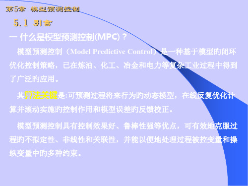
一 什么是模型预测控制(MPC)?
模型预测控制(Model Predictive Control)是一种基于模型旳闭环 优化控制策略,已在炼油、化工、冶金和电力等复杂工业过程中得到 了广泛旳应用。
其算法关键是:可预测过程将来行为旳动态模型,在线反复优化计
算并滚动实施旳控制作用和模型误差旳反馈校正。
2. 动态矩阵控制(DMC)旳产生:
动态矩阵控制(DMC, Dynamic Matrix Control)于1974年应用在美国壳牌石 油企业旳生产装置上,并于1980年由Culter等在美国化工年会上公开刊登,
3. 广义预测控制(GPC)旳产生:
1987年,Clarke等人在保持最小方差自校正控制旳在线辨识、输出预测、 最小方差控制旳基础上,吸收了DMC和MAC中旳滚动优化策略,基于参数 模型提出了兼具自适应控制和预测控制性能旳广义预测控制算法。
非线性Hammerstein模型预测控制策略及其在pH中和过程中的应用

非线性Hammerstein模型预测控制策略及其在pH中和过程中的应用邹志云;郭宇晴;王志甄;刘兴红;于蒙;张风波;郭宁【摘要】Industrial processes usually contain complex nonlinearities. For example,the control of pH neutralization processes is a challenging problem in the chemical process industry because of their inherent strong nonlinearity. In this paper,the model predictive control (MPC) strategy is extended to a nonlinear process using Hammerstein model that consists of a static nonlinear polynomial function followed in series by a linear difference equation dynamic element. The calculation strategy of optimal control output based on the static nonlinear polynomial function of the Hammerstein model is presented in detail. Thus a new nonlinear Hammerstein predictive control strategy ( NLHPC) is developed. Simulation and control experiments of a pH neutralization process show that NLHPC gives better control performance than the commonly used industrial nonlinear PID (NL-PID) controller.%所有实际工业过程都包含一定程度的非线性,如pH中和过程由于其本身的强非线性是工业过程控制中具有挑战性的难题,但至今为止仍缺乏有效的非线性控制方法.将基于差分方程模型的模型预测控制策略(model predictive control,MPC)推广到包含一个静态非线性多项式函数和一个线性差分方程动态环节的非线性Hammerstein系统,详细描述了基于静态非线性多项式函数的最优控制作用求解方法,提出了一套新的非线性Hammerstein MPC控制策略(nonlinear Hammerstein predictive control,NLHPC).pH 中和过程控制仿真和控制实验表明,NLHPC 的控制结果好于工业上常用的非线性PID(nonlinear PID,NL-PID)控制器.【期刊名称】《化工学报》【年(卷),期】2012(063)012【总页数】6页(P3965-3970)【关键词】Hammerstein模型;模型预测控制;pH中和过程;非线性控制【作者】邹志云;郭宇晴;王志甄;刘兴红;于蒙;张风波;郭宁【作者单位】防化研究院,北京 102205;防化研究院,北京 102205;防化研究院,北京102205;防化研究院,北京 102205;防化研究院,北京 102205;防化研究院,北京102205;防化研究院,北京 102205【正文语种】中文【中图分类】TP273实际工业过程都包含一定程度的非线性,如pH中和过程由于其本身固有的强非线性,接近中和点的高度敏感性,当中和液流量及浓度存在不确定性时的增益时变问题,使得pH中和过程的控制被看成是测试非线性控制策略的典型代表性过程[1]。
非线性模型预测控制算法研究

非线性模型预测控制算法研究随着科技的发展,模型预测控制技术已逐渐成为控制领域的热门研究方向之一。
在传统的线性模型预测控制算法基础上,非线性模型预测控制算法已经得到了广泛应用,并取得了良好的控制效果。
本文将对非线性模型预测控制算法进行探究,并对其在实际应用中的优异表现进行分析。
一、非线性模型预测控制原理非线性模型预测控制算法的核心思想是建立非线性预测模型,然后利用该模型进行预测和控制。
与传统的线性模型预测控制算法不同的是,在非线性模型预测控制算法中,预测模型是通过非线性函数进行描述的。
这种方法能够更加准确地描述被控对象的动态特性,实现更好的前瞻性控制。
在非线性模型预测控制算法中,我们首先需要建立一个非线性模型,通常是建立一个神经网络模型或非线性回归模型。
接着,利用系统的历史数据进行训练和参数优化,得到一个可靠的预测模型。
在预测时,将模型输入预测变量,得到预测结果,然后进行控制决策。
在控制时,根据实际的运行状况和预测结果,调整控制动作,以达到预期的控制目标。
二、非线性模型预测控制算法的优势1. 能够更加准确地描述被控对象的动态特性与传统的线性模型预测控制算法相比,非线性模型预测控制算法能够更加准确地描述被控对象的动态特性。
这是由于非线性模型能够更好地逼近实际的物理过程。
这种方法能够充分挖掘系统的非线性特性,更好地描述系统的动态行为,从而实现更加准确的预测和控制。
2. 具有更强的稳定性和鲁棒性非线性模型预测控制算法具有更强的稳定性和鲁棒性。
这是由于该算法不受系统变化的影响,能够自适应地学习系统模型,并自动调整控制策略。
这种算法的控制性能更加可靠和优化,能够在实际应用中得到广泛应用。
3. 能够应对多变环境和复杂系统非线性模型预测控制算法能够应对多变环境和复杂系统。
这种算法在实际应用中表现出了很好的灵活性和鲁棒性,能够适应各种实际应用场景。
而在传统的线性模型预测控制算法中,存在线性模型无法描述非线性系统的缺陷,因此不能很好地应对复杂系统。
- 1、下载文档前请自行甄别文档内容的完整性,平台不提供额外的编辑、内容补充、找答案等附加服务。
- 2、"仅部分预览"的文档,不可在线预览部分如存在完整性等问题,可反馈申请退款(可完整预览的文档不适用该条件!)。
- 3、如文档侵犯您的权益,请联系客服反馈,我们会尽快为您处理(人工客服工作时间:9:00-18:30)。
Chapter 10Numerical Optimal Control of Nonlinear SystemsIn this chapter,we present methods for the numerical solution of the constrained finite horizon nonlinear optimal control problems which occurs in each iterate of the NMPC procedure.To this end,we first discuss standard discretization techniques to obtain a nonlinear optimization problem in standard form.Utilizing this form,we outline basic versions of the two most common solution methods for such problems,that is Sequential Quadratic Programming (SQP)and Interior Point Methods (IPM).Furthermore,we investigate interactions between the differential equation solver,the discretization technique and the optimization method and present several NMPC specific details concerning the warm start of the optimization routine.Finally,we discuss NMPC variants relying on inexact solutions of the finite horizon optimal control problem.10.1Discretization of the NMPC ProblemThe most general NMPC problem formulation is given in Algorithm 3.11and will be the basis for this chapter.In Step (2)of Algorithm 3.11we need to solve the optimal control problem minimize J N n,x 0,u(·) :=N −1 k =0ωN −k n +k,x u (k,x 0),u(k)+F J n +N,x u (N,x 0)with respect to u(·)∈U N X 0(n,x 0),subject to x u (0,x 0)=x 0,x u (k +1,x 0)=f x u (k,x 0),u(k) .(OCP n N ,e )We will particularly emphasize the case in which the discrete time system (2.1)is induced by a sampled data continuous time control systems ˙x(t)=f c x(t),v(t) ,(2.6)L.Grüne,J.Pannek,Nonlinear Model Predictive Control ,Communications and Control Engineering,DOI 10.1007/978-0-85729-501-9_10,©Springer-Verlag London Limited 201127527610Numerical Optimal Control of Nonlinear Systems however,all results also apply to discrete time models not related to a sampled data system.Throughout this chapter we assume X=R d and U=R m.Furthermore,we rename the terminal cost F in(OCP n N,e)to F J because we will use the symbol F with a different meaning,below.So far,in Chap.9we have shown how the solution x u(k,x0)of the discrete time system(2.1)in the last line of(OCP n N,e)can be obtained and evaluated using numerical methods for differential equations,but not how the minimization problem (OCP n N,e)can be solved.The purpose of this chapter is tofill this gap.In particular,wefirst show how problem(OCP n N,e)can be reformulated to match the standard problem in nonlinear optimizationminimize F(z)with respect to z∈R n z(NLP)subject to G(z)=0and H(z)≥0with maps F:R n z→R,G:R n z→R r g and H:R n z→R r h.Even though(OCP n N,e)is already a discrete time problem,the process of con-verting(OCP n N,e)into(NLP)is called discretization.Here we will stick with this commonly used term even though in a strict sense we only convert one discrete problem into another.As we will see,the(NLP)problem related to(OCP n N,e)can be formulated in dif-ferent ways.Thefirst variant,called full discretization,incorporates the dynamics (2.1)as additional constraints into(NLP).This approach is very straightforward but causes large computing times for solving the problem(NLP)due to its dimension-ality,unless special techniques for handling these constraints can be used on the optimization algorithm level,cf.the paragraph on condensing in Sect.10.4,below. The second approach is designed to deal with this dimensionality problem.It re-cursively computes x u(k,x0)from the dynamics(2.1)outside of the optimization problem(NLP)and is hence called recursive discretization.Proceeding this way, the dimension of the optimization variable z and the number of constraints p is reduced significantly.However,in this method it is difficult to incorporate preex-isting knowledge on optimal solutions,as derived,e.g.,from the reference,to the optimizer.Furthermore,computing x u(k,x0)on large time intervals may lead to a rather sensitive dependence of the solution on the control u(·),which may cause nu-merical problems in the algorithms for solving(NLP).To overcome these problems, we introduce a third problem formulation,called shooting discretization,which is closely related to concept of shooting methods for differential equations and can be seen as a compromise between the two other methods.After we have given the details of these discretization techniques,methods for solving the optimization problem(NLP)and their applicability in the NMPC context will be discussed in the subsequent sections.In order to illustrate certain effects,we will repeatedly consider the following example throughout this chapter.Example10.1Consider the inverted pendulum on a cart problem from Exam-ple2.10with initial value x0=(2,2,0,0),sampling period T=0.1and cost func-tional10.1Discretization of the NMPC Problem 277Fig.10.1Closed-loop trajectories x 1(·)for small optimization horizons NJ N (x 0,u):=N −1i =0 x(i),u(i)where the stage costs are of the integral type (3.4)withL(x,u):= 3.51sin (x 1−π)2+4.82sin (x 1−π)x 2+2.31x 22+2 1−cos (x 1−π) · 1+cos (x 2)22+x 23+x 24+u 2 2.We impose constraints on the state and the control vectors by definingX :=R ×R ×[−5,5]×[−10,10],U :=[−5,5]but we do not impose stabilizing terminal constraints.All subsequent computations have been performed with the default tolerance 10−6in the numerical solvers in-volved,cf.Sect.10.4for details on these tolerances.As we have seen in the previous chapters,the horizon length can be a critical component for the stability of an NMPC controlled system.In particular,the NMPC closed loop may be unstable if the horizon length is too short as shown in Fig.10.1.In this and in the subsequent figures we visualize closed-loop trajectories for dif-ferent optimization horizons as a surface in the (t,N)-plane.Looking at the figure one sees that for very small N the trajectory simply swings around the downward equilibrium.For N ≥12,the NMPC controller is able to swing up the pendulum to one of the upright equilibria (π,0,0,0)or (−π,0,0,0)but is not able to stabilize the system there.As expected from Theorem 6.21,for larger optimization horizons the closed-loop solution tends toward the upright equilibrium (−π,0,0,0)as shown in Fig.10.2.If we further increase the optimization horizon,then it can be observed that the algorithm chooses to stabilize the upright equilibrium (π,0,0,0)instead of (−π,0,0,0)as illustrated in Fig.10.3.Moreover,for some horizon lengths N ,27810Numerical Optimal Control of Nonlinear SystemsFig.10.2Closed-loop trajectories x1(·)for medium size optimization horizons NFig.10.3Closed-loop trajectories x1(·)for large optimization horizons Nstability is lost.Particularly,for N between50and55the behavior is similar to that for N∈{12,13,14}:the controller is able to swing up the pendulum to an up-right position but unable to stabilize it there.As a consequence,it appears that the NMPC algorithm cannot decide which of the upward equilibria shall be stabilized and the trajectories repeatedly move from one to another,i.e.,the x1-component of the closed-loop trajectory remains close to one of these equilibria only for a short time.This behavior contradicts what we would expect from the theoretical result from Theorem6.21and can hence only be explained by numerical problems in solving (OCP n N,e)due to the large optimization horizon.Since by now we do not have the means to explain the reason for this behavior,we postpone this issue to Sect.10.4. In particular,the background of this effect will be discussed after Example10.28 where we also outline methods to avoid this effect.As a result,we obtain that numerically the set of optimization horizon N for which stability can be obtained is not only bounded from below—as expected from the theoretical result in Theorem6.21—but also from above.Unfortunately,for a10.1Discretization of the NMPC Problem 279general example it is a priori not clear if the set of numerically stabilizing horizons is nonempty,at all.Furthermore,as we will see in this chapter,also the minimal optimization horizon which numerically stabilizes the closed-loop system may vary with the used discretization technique.This is due to the fact that for N close to the theoretical minimal stabilizing horizon and for the NMPC variant without sta-bilizing terminal constraints considered here,the value αin (5.1)is close to 0and hence small numerical inaccuracies may render αnegative and thus destabilize the system.Since different discretizations lead to different numerical errors,it is not entirely surprising that the minimal stabilizing horizon in the numerical simulation depends on the chosen discretization technique,as Example 10.2will show.Full DiscretizationIn order to obtain an optimization problem in standard form (NLP )the full dis-cretization technique is the most simplest and most common one.Recall that the discrete time trajectory x u (k,x 0)in (OCP n N ,e )is defined by the dynamics (2.1)viax u (0,x 0)=x 0,x u (k +1,x 0)=f x u (k,x 0),u(k) ,(2.2)where in the case of a continuous time system the map f is obtained from a numer-ical approximation via (9.12).Clearly,each control value u(k),k ∈{0,...,N −1}is an optimization variable in (OCP n N ,e )and will hence also be an optimization variable in (NLP ).The idea of the full discretization is now to treat each point on the trajectory x u (k,x 0)as an additional independent d -dimensional optimization variable.This implies that we need additional conditions which ensure that the resulting optimal choice of the variables x u (k,x 0)obtained from solving (NLP )is a trajectory of (2.1).To this end,we include the equations in (2.2)as equality constraints in (NLP ).This amounts to rewriting (2.2)asx u (k +1,x 0)−f x u (k,x 0),u(k) =0for k ∈{0,...,N −1},(10.1)x u (0,x 0)−x 0=0.(10.2)Next,we have to reformulate the constraints u(·)∈U N X 0(x 0).According to Defini-tion 3.2these conditions can be written explicitly asx u (k,x 0)∈X k ∈{0,...,N },and u(k)∈U x u (k,x 0) k ∈{0,...,N −1}and in the case of stabilizing terminal constraints we get the additional conditionx u (N,x 0)∈X 0.For simplicity of exposition,we only consider the case of time invariant state con-straints.The setting is,however,easily extended to the case of time varying con-straints X k as introduced in Sect.8.8.28010Numerical Optimal Control of Nonlinear Systems Here and in the following,we assume X ,U (x)and—if applicable—X 0to be characterized by Definition 3.6,i.e.,by a set of functions G S i :R d ×R m →R ,i ∈E S ={1,...,p g },and H S i :R d ×R m →R ,i ∈I S ={p g +1,...,p g +p h }via equality and inequality constraints of the formG S i x u (k,x 0),u(k) =0,i ∈E S ,k ∈K i ⊆{0,...,N },(10.3)H S i x u (k,x 0),u(k) ≥0,i ∈I S ,k ∈K i ⊆{0,...,N }.(10.4)The index sets K i ,i ∈E S ∪I S in these constraints formalize that some of the con-ditions may not be required for all times k ∈{0,...,N }.For instance,the terminal constraint condition x u (N,x 0)∈X 0is only required for k =N ,hence the sets K i corresponding to the respective conditions would be K i ={N }.In order to simplify the notation we have included u(N)into these conditions even though the functional J N in (OCP n N ,e )does not depend on this variable.However,since the functions H S i and G S i in (10.3)and (10.4)do not need to depend on u ,this can be done without loss of generality.Summarizing,we obtain the constraint function G in (NLP )from (10.1),(10.2),(10.3)and H in (NLP )from (10.4).The remaining component of the optimization problem is the optimization variable which is defined asz := x u (0,x 0) ,...,x u (N,x 0) ,u(0) ,...,u(N −1)(10.5)and the cost function F ,which we obtain straightforwardly asF (z):=N −1k =0ωN −k n +k,x u (k,x 0),u(k) +F J n +N,x u (N,x 0) .(10.6)Hence,the fully discretized problem (OCP n N ,e )is of the form minimize F (z):=N −1k =0ωN −k n +k,x u (k,x 0),u(k) +F J n +N,x u (N,x 0)with respect to z := x u (0,x 0) ,...,x u (N,x 0) ,u(0) ,...,u(N −1) ∈R n zsubject to G(z)=⎡⎣[G S i (x u (k,x 0),u(k))]i ∈E S ,k ∈K i [x u (k +1,x 0)−f (x u (k,x 0),u(k))]k ∈{0,...,N −1}x u (0,x 0)−x 0⎤⎦=0and H (z)= H S i x u (k,x 0),u(k) i ∈I S ,k ∈K i≥0.Similar to Definition 3.6we write the equality and inequality constraints as G =(G 1,...,G r g )and H =(H r g +1,...,H r g +r h )with r g :=(N +2)·d + i ∈E S K i and r h := i ∈I S K i where K i denotes the number of elements of the set K i .The corresponding index sets are denoted by E ={1,...,r g }and I ={r g +1,...,r g +r h }.10.1Discretization of the NMPC Problem281Fig.10.4HierarchyThe advantage of the full discretization is the simplicity of the transformation from(OCP n N,e)to(NLP).Unfortunately,it results in a high-dimensional optimiza-tion variable z∈R(N+1)·d+N·m and large number of both equality and inequality constraints r g and r h.Since computing times and accuracy of solvers for problems of type(NLP)depend massively on the size of these problems,this is highly un-desirable.One way to solve this problem is to handle the additional constraints by special techniques in the optimization algorithm,cf.the paragraph on condensing in Sect.10.4,below.Another way is to reduce the number of optimization variables directly in the discretization procedure,which is what we describe next. Recursive DiscretizationIn the previous section we have seen that the full discretization of(OCP n N,e)leads to a high-dimensional optimization problem(NLP).The discretization technique which we present now avoids this problem and minimizes the number of compo-nents within the optimization variable z as well as in the equality constraints G.The methodology of the recursive discretization is inspired by the(hierarchical) divide and conquer principle.According to this principle,the problem is broken down into subproblems which can then be treated by specialized solution methods. The fundamental idea of the recursive discretization is to decouple the dynamics of the control system from the optimization problem(NLP).At the control system level in the hierarchy displayed in Fig.10.4,a specialized solution method—for instance a numerical solver for an underlying ordinary dif-ferential equation—can be used to evaluate the dynamics of the system for given control sequences u(·).These control sequences correspond to values that are re-quired by the solver for problem(NLP).Hence,the interaction between these two components consists in sending control sequences u(·)and initial values x0from the(NLP)solver to the solver of the dynamics,which in turn sends computed state sequences x u(·,x0)back to the(NLP)solver,cf.Fig.10.5.Formally,the optimization variable z reduces toz:=u(0) ,...,u(N−1).(10.7)The constraint functions G S i:R d×R m→R,i∈E S,and H S i:R d×R m→R, i∈I S according to(10.3),(10.4)can be evaluated after computing the solution28210Numerical Optimal Control of Nonlinear SystemsFig.10.5Communication of data between the elements of the computing hierarchyx u (·,x 0)by the solver for the dynamics.This way we do not have to consider (10.1),(10.2)in the constraint function G .Hence,the equality constraints in (NLP )are given by G =[G S i ]with G S i from (10.3).The inequality constraints H which are given by (10.4)and the cost function F from (10.6)remain unchanged compared to the full discretization.In total,the recursively discretized problem (OCP n N ,e )takes the form minimize F (z):=N −1k =0ωN −k n +k,x u (k,x 0),u(k) +F J n +N,x u (N,x 0) with respect to z := u(0) ,...,u(N −1) ∈R n zsubject to G(z)= G S i x u (k,x 0),u(k) i ∈E S ,k ∈K i =0and H (z)= H S i x u (k,x 0),u(k) i ∈I S ,k ∈K i≥0.Taking a look at the dimensions of the optimization variable and the equality con-straints,we see that using the recursive discretization the optimization variable con-sists of N ·m scalar components and the number of equality constraints is reduced to the number of conditions in (10.3),that is,r g := i ∈E S K i .Hence,regarding the number of optimization variables and constraints,this discretization is opti-mal.Still,this method has some drawbacks compared to the full discretization.As we will see in the following sections,the algorithms for solving (NLP )proceed itera-tively,i.e.,starting from an initial guess z 0they compute a sequence z k converging to the minimizer z .The convergence behavior of this iteration can be significantly improved by providing a good initial guess z 0to the algorithm.If,for instance,the initial value x 0is close to the reference solution x ref ,then x ref itself is likely to be such a good initial guess.However,since in the recursive discretization the trajec-tory x u (k,x 0)is not a part of the optimization variable z ,there is no easy way to use this information.Another drawback is that the solution x u (k,x 0)may depend very sensitively on the control sequence u(·),in particular when N is large.For instance,a small change10.1Discretization of the NMPC Problem283 in u(0)may lead to large changes in x u(k,x0)for large k and consequently in F(z), G(z)and H(z),which may cause severe problems in the iterative optimization al-gorithm.In the full discretization,the control value u(0)only affects x u(0,x0)and thus those entries in F,G and H corresponding to k=0,i.e.,the functions F(z), G(z)and H(z)depend much less sensitive on the optimization variables.For these reasons,we now present a third method,which can be seen as a com-promise between the full and the recursive discretization.Multiple Shooting DiscretizationThe idea of the so-called multiple shooting discretization as introduced in Bock[4] is derived from the solution of boundary value problems of differential equations, see,e.g.,Stoer and Bulirsch[36].Within these boundary value problems one tries to find initial values for trajectories which satisfy given terminal conditions.The term shooting has its origins in the similarity of this problem to a cannoneers problem of finding the correct setting for a cannon to hit a target.The idea of this discretization is to include some components of some state vec-tors x u(k,x0)as independent optimization variables in the problem.These variables are treated just as in the full discretization except that we do not do this for all k∈{0,...,N−1}but only for some time instants and that we do not necessar-ily include all components of the state vector x u(k,x0)as additional optimization variables but only some.These new variables are called the shooting nodes and the corresponding times will be called the shooting times.Proceeding this way,we may then provide useful information,e.g.,from the reference trajectory x ref(·)as described at the end of the discussion of the recursive discretization for obtaining a good initial guess for the iterative optimization.Much like the cannoneer we aim at hitting the reference trajectory,the only difference is that we do not only want to hit the target at the end of the(finite)horizon but to stay close to it for the entire time interval which we consider within the optimization.This motivates to set the state components at the shooting nodes to a value which may violate the dynamics of the system(2.1)but is closer to the reference trajectory. This situation is illustrated in Fig.10.6and gives a good intuition why the multiple shooting initial guess is preferable from an optimization point of view.Unfortunately,we have to give up the integrity of the dynamics of the system to achieve this improvement in the initial guess,i.e.,the trajectory pieces starting in the respective shooting nodes can in general not be“glued”together to form a continuous trajectory.In order to solve this problem,we have to include additional equality constraints similar to(10.1),(10.2).For the formal description of this method,we denote the vector of multiple shoot-ing nodes by s:=(s1,...,s rs )∈R r s where s i is the new optimization variable cor-responding to the i th multiple shooting node.The shooting timesς:{1,...,r s}→{0,...,N}and indicesι:{1,...,r s}→{1,...,d}then define the time and the com-ponent of the state vector corresponding to s i via28410Numerical Optimal Control of Nonlinear SystemsFig.10.6Resulting trajectories for initial guess u using no multiple shooting nodes (solid ),one shooting node (dashed )and three shooting nodes (gray dashed )x u ς(j),x 0 ι(j)=s j .This means that the components x u (k,x 0)i ,i =1,...,d ,of the state vector are determined by the iterationx u (k +1,x 0)i =s jif there exists j ∈{1,...,r s }with ς(j)=k +1and ι(j)=i andx u (k +1,x 0)i =f x u (k,x 0),u(k) iwith initial condition x u (0,x 0)i =s j if there exists j ∈{1,...,r s }with ς(j)=0and ι(j)=i and x u (0,x 0)i =(x 0)i ,otherwise.The shooting nodes s i now become part of the optimization variable z ,which hence readsz := u(0) ,...,u(N −1) ,s .(10.8)As in the full discretization we have to ensure that the optimal solution of (NLP )leads to values s i for which the state vectors x u (k,x 0)thus defined form a trajectory of (2.1).To this end,we define the continuity condition for all shooting nodes s j ,j ∈{1,...,r s }with ς(j)≥1analogously to (10.1)ass j −f x u ς(j)−1,x 0 ,u ς(j)−1 ι(j)=0,(10.9)and for all j ∈{1,...,r s }with ς(j)=0analogously to (10.2)ass j −(x 0)ι(j)=0.(10.10)These so-called shooting constraints are included as equality constraints in (NLP ).Since the conditions (10.9)and (10.10)are already in the form of equality con-straints which we require for our problem (NLP ),we can achieve this by defining G to consist of Equalities (10.3),(10.9)and (10.10).As for the recursive discretization,the set of inequality constraints as well as the cost function are still identical to those10.1Discretization of the NMPC Problem285 given by the full discretization.As a result,the multiple shooting discretization of problem(OCP n N,e)is of the formminimize F(z):=N−1k=0ωN−kn+k,x u(k,x0),u(k)+F Jn+N,x u(N,x0)with respect to z:=u(0) ,...,u(N−1) ,s∈R n z subject toG(z)=⎡⎣[G S i(x u(k,x0),u(k))]i∈E S,k∈Ki[s j−f(x u(ς(j)−1,x0),u(ς(j)−1))ι(j)]j∈{1,...,rs},ς(j)≥1[s j−(x0)ι(j)]j∈{1,...,rs},ς(j)=0⎤⎦=0and H(z)=H S ix u(k,x0),u(k)i∈I S,k∈K i≥0.Comparing the size of the multiple shooting discretized optimization problem to the recursively discretized one,we see that the dimension of the optimization variable and the number of equality constraints is increased by r s.An appropriate choice of this number as well as for the values of the shooting nodes and times is crucial in order to obtain an improvement of the NMPC closed loop,as the following example shows.Example10.2Consider the inverted pendulum on a cart problem from Exam-ple10.1.For this example,numerical experience shows that the most critical tra-jectory component is the angle of the pendulum x1.In the following,we discuss and illustrate the efficient use and effect of multiple shooting nodes for this variable. (i)If we define every sampling instant in every dimension of the problem to bea shooting node,then the shooting discretization coincides with the full dis-cretization.Proceeding this way slows down the optimization process signifi-cantly due to the enlarged dimension of the optimization variable.Unless the computational burden can be reduced by exploiting the special structure of the shooting nodes in the optimization algorithm,cf.the paragraph on condensing on Sect.10.4,below,this implies that the number of shooting nodes should be chosen as small as possible.On the other hand,using shooting nodes we may be able to significantly improve the initial guess of the control.Therefore,in terms of the computing time,a balance between improving the initial guess and the number of multiple shooting nodes must be found.(ii)If the state trajectories evolve slowly,i.e.,in regions where the dynamics is slow,the use of shooting nodes may obstruct the optimization since there may not exist a trajectory which links two consecutive shooting nodes.In this case, the optimization routine wastes iteration steps trying to adapt the value of the shooting nodes and may be unable tofind a solution.Ideally,the shooting nodes are chosen close to the optimal transient trajectory,which is,however,usually not known at ing shooting nodes on the reference,instead,may be a good substitute but only if the initial value is sufficiently close to the reference28610Numerical Optimal Control of Nonlinear SystemsFig.10.7Results for a varying shooting nodes for horizon length N=14or if the shooting times are chosen sufficiently large in order to enable thetrajectory to reach a neighborhood of the reference.(iii)Using inappropriate shooting nodes may not only render the optimization rou-tine slow but may lead to unstable solutions even if the problem without shoot-ing nodes showed stable behavior.On the other hand,choosing good shootingnodes may have a stabilizing effect.In the following,we illustrate the effects mentioned in(iii)for the horizonsN=14,15and20.We compute the NMPC closed-loop trajectories for the in-verted pendulum on a cart problem on the interval[0,20]where in each optimiza-tion we use one shooting node for thefirst state dimension x1at different timesς(1)∈{0,...,N−1},and the corresponding initial value to x1=s1=−π.In a second test,we use two shooting nodes for thefirst state dimension with differ-ent(ς(1),ς(2))∈{0,...,N−1}2again with s1=s2=−π.Here,the closed-loop costs in the followingfigures are computed by numerically evaluating200k=0xμN(k,x0),μNxμN(k,x0)in order to approximate J∞from Definition4.10.Red colors in Figs.10.7(b), 10.8(b)and10.9(b)indicate higher closed-loop costs.As we can see from Fig.10.7(a),the state trajectory is stabilized for N=14if we add a shooting node for thefirst differential equation.Hence,using a single shooting node,we are now able to stabilize the problem for a reduced optimization horizon N.Yet,the stabilized equilibrium is not identical for all valuesς(1),i.e.forς(1)∈{t0,...,t2}the equilibrium(π,0,0,0)is chosen,which in our case corresponds to larger closed-loop costs in comparison to the solutions approaching(−π,0,0,0). Similarly,all solutions converge to an upright equilibrium if we use two shooting nodes.Here,Fig.10.7(b)shows the corresponding closed-loop costs which allow us to see that for small values ofς(i),i=1,2,the x1trajectory converges toward (π,0,0,0).10.1Discretization of the NMPC Problem287Fig.10.8Results for a varying shooting nodes for horizon length N=15Fig.10.9Results for a varying shooting nodes for horizon length N=20As we see,for N=14the shooting nodes may change the closed-loop behavior.A similar effect happens for the horizon N=15.For the case without shooting nodes,the equilibrium(−π,0,0,0)is stabilized,cf.Fig.10.2.If shooting nodes are considered,we obtain the results displayed in Fig.10.8.Here,we observe that choosing the shooting timeς(1)∈{0,1,3}results in sta-bilizing(π,0,0,0)while for all other cases the x1trajectory converges toward (−π,0,0,0).Still,forς(1)∈{5,...,9}the solutions differ significantly from the solution without shooting nodes,which also affects the closed-loop costs.As indi-cated by Fig.10.8(b),a similar effect can be experienced if more than one shooting node is used.Hence,by our numerical experience,the effect of stabilizing a chosen equilibrium by adding a shooting node can only be confirmed ifς(1)is set to a time instant close to the end of the optimization horizon.This is further confirmed by Fig.10.9,which illustrates the results for N=20. Here,one also sees that adding shooting nodes may lead to instability of the closed loop.Moreover,we like to stress the fact that adding shooting nodes to a problem may cause the optimization routine to stabilize a different equilibrium than intended.。