数字信号处理(第四版)第四章ppt
合集下载
《数字信号处理》课件第4章 (2)

(4-6b)
j 1
V jk (z) Fjk (z)W j (z)
(4-7)
相应的信号流图如图4.8所示。
第四章 数字滤波器的结构表示
源节 点1 1 X(z)或x(n)
a
2
3
z- 1 b
4
吸收 节点 1 Y(z)或y(n)
图4.8 标有支路传输比的Z变换形式的流图
第四章 数字滤波器的结构表示
在图4.8中,每一个支路的传输比均列于该支路的箭头之侧。 对支路(2、4)而言,它所作的是单位延迟变换, 此时的传递
第四章 数字滤波器的结构表示
第四章 数字滤波器的结构表示
4.1 引言 4.2 数字滤波器的信号流图表示 4.3 数字网络的矩阵表示 4.4 无限冲激响应(IIR)系统的基本网络结构 4.5 转置型 4.6 有限冲激响应(FIR)系统的基本网络结构
第四章 数字滤波器的结构表示
4.1 引 言
在设计数字滤波器的过程中,通常总是根据工程指标,按一 定的设计方法或技术,正确确定能够满足所需指标要求的滤波器 的数学模型,然后利用计算机或专用硬件加以实现。为了论述方 便, 我们把滤波器数学模型的确定放到第六章数字滤波器的设计 方法中专门研究,而把数学模型的具体实现放在这里先作必要的 介绍。 而且在这一章中,我们只对该数学模型的硬件实现作必要 的讨论, 利用计算机实现的软件设计则不再赘述。
第四章 数字滤波器的结构表示
S jk (z) bjk X j (z) Rjk (z) c jkWj (z)
把它们代入式(4-6),
N
M
Wk (z) Fjk (z)Wj (z) bjk X j (z)
j 1
j 1
N
Yk (z) c jkWj (z) j 1
数字信号处理(第四版)第四章ppt

Digital Signal Processing
© 2013 Jimin Liang
Discrete-Time Systems Outline Discrete-time system examples Classification of DT systems Impulse and step responses Time-domain characteristics of LTI Simple interconnection schemes
Process a given sequence, called the input system, to generate another sequence, called the output sequence, with more desirable properties or to extract certain information about the input signal. DT system is usually also called the digital filter
12
Digital Signal Processing
© 2013 Jimin Liang
Discrete-Time Systems 4.2 Classification of DT systems Stable system
A system is stable if and only if for every bounded input, the output is also bounded, called BIBO stable.
Discrete-Time Systems 4.1 Discrete-time system examples (4) Linear Interpolator Linear factor-2 interpolator
数字信号处理第四章快速傅里叶变换PPT课件
2N (2N – 1)
复乘的加
法次数
4
4.2 FFT:直接计算 DFT 的问题及改进
如 N=512、1024 和 8192 时,DFT 的乘法运算 N2 = 5122 = 218 = 262144(26万次) N2 = 10242 = 220 = 1048576(105万次) N2 = 81922 = 226 = 67108864(6千7百万次)
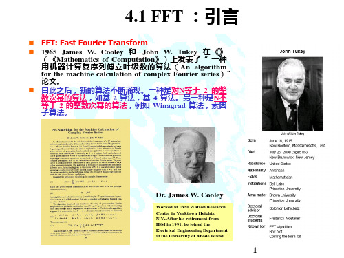
Dr. James W. Cooley
Worked at IBM Watson Research Center in Yorktown Heights, N.Y..After his retirement from IBM in 1991, he joined the Electrical Engineering Department at the University of Rhode Island.
x(0)
x(2)
-1
x(1)
x(3)
-1 W41
X(0) X(0)x(0) x(2)x(1) x(3)
X(1) X(1)x(0) x(2)x(1) x(3)W41 只需要 1
-1 X(2) X(2)x(0) x(2)x(1) x(3)
次复数乘
-1
X(3) X(3)x(0) x(2)x(1) x(3)W41
4.1 FFT :引言
FFT: Fast Fourier Transform 1965 James W. Cooley 和 John W. Tukey 在 《》
(《Mathematics of Computation》)上发表了“ 一种 用机器计算复序列傅立叶级数的算法(An algorithm for the machine calculation of complex Fourier series)” 论文。 自此之后,新的算法不断涌现。一种是对N等于 2 的整 数次幂的算法,如基 2 算法,基 4 算法。另一种是N不 等于 2 的整数次幂的算法,例如 Winagrad 算法,素因 子算法。
数字信号处理课件第四章资料

k 0,1,..., N 1 2
5、时间抽取蝶形运算流图符号
X1(k)
X1(k) WNk X 2 (k)
X 2 (k )
WNk
1 X1(k) WNk X 2 (k)
返回DIF 返回例题
设 N 23 8
X1(k)
X 2 (k )
WNk
k 0
W80
1
W81
2
W82
3
W83
X (k)
k 0,1,,7
l0
l 0
X1(k) X 3(k) WNk X 4 (k)
2
X1(k
N 4
)
X 3 (k )
W Nk
2
X
4
(k)
k 0,1,..., N 1 4
x2(r)也进行同样的分解:
x5 (l) x2 (2l)
x6 (l) x2 (2l 1)
l 0,1,..., N 1 4
)
N
/ 21
x1(r)WNrk/ 2
X1(k)
r 0
r 0
X2(k N / 2) X2(k) X (k) X1(k) WNk X 2 (k)
W (kN N
/
2)
WNkWNN
/
2
WNk
N点X(k)可以表示成前 N点和后 点N 两部分:
2
2
前半部分X(k):
X (k) X1(k) WNk X 2 (k)
N 1
X (k) x(n)WNnk k = 0, 1, …, N-1
n0
x(n)
1 N
N 1
X (k )WNnk
k 0
n = 0, 1, …, N-1
二者的差别只在于WN 的指数符号不同,以及差一 个常数因子1/N,所以IDFT与DFT具有相同的运算量。
数字信号处理-原理、实现及应用(第4版) 第四章 模拟信号的数字处理

(3)当未知时,由 x(n) 无法恢复原正弦信号。
结论:
正弦信号采样(2)
三点结论: (1)对正弦信号,若 Fs 2 f0 时,不能保证从采样信号恢
复原正弦信号; (2)正弦信号在恢复时有三个未知参数,分别是振幅A、
频率f和初相位,所以,只要保证在一个周期内均匀采样 三点,即可由采样信号准确恢复原正弦信号。所以,只要 采样频率 Fs 3 f0 ,就不会丢失信息。 (3)对采样后的正弦序列做截断处理时,截断长度必须 是此正弦序列周期的整数倍,才不会产生频谱泄漏。(见 第四章4.5.3节进行详细分析)。
D/A
D/A为理想恢复,相当于理想的低通滤波器,ya (t) 的傅里叶变换为:
Ya ( j) Y (e jT )G( j) H (e jT ) X (e jT )G( j)
保真系统中的应用。
在 |Ω|>π/T ,引入了原模拟信号没有的高频分量,时域上表现
为台阶。
ideal filter
•
-fs
-fs/2 o
• fs/2 fs
f •
2fs
•
•
-fs
-fs/2 o
fs/2
•
fs
•
f
2fs
措施
D/A之前,增加数字滤波器,幅度特性为 Sa(x) 的倒数。
在零阶保持器后,增加一个低通滤波器,滤除高频分量, 对信号进行平滑,也称平滑滤波器。
c
如何恢复原信号的频谱?
P (j)
加低通滤波器,传输函数为
G(
j)
T
0
s 2 s 2
s
0
s
X a ( j)
s 2
s c c
s
理想采样的恢复
《数字信号处理教学课件》第四章 快速傅立叶变换
k
)
k 0,1,...... N 4 1
注意:通常我们会把
WNk
/
写成
2
W
2k N
。
N点DFT的第二次时域抽取分解图(N=8)
x(0)
x(4) x(2) x(6) x(1) x(5) x(3) x(7)
x(0) xD2(F2点)T
X3(0) X3(1)
4点
x2(4点) xD(F6)T
x2(1点) xD(F3)T
分解后的运算量:
一个N 点DFT 一个N / 2点DFT 两个N / 2点DFT
一个蝶形 N / 2个蝶形
总计
复数乘法 N2
(N / 2)2 N2/ 2
1 N/2 N2/2 + N/2 ≈ N2/2
运算量减少了近一半
复数加法 N (N–1) N / 2 (N / 2 –1) N (N / 2 –1)
x(1),x(3),x(5),x(7)为奇子序列 频域上:X(0)~X(3),由X(k)给出
X(4)~X(7),由X(k+N/2)给出
N=8点的直接DFT的计算量为: 复乘:N2次 = 64次 复加:N(N-1)次 = 8×7=56次
X (k )
X
1
(k
)
W
k N
X2(k)
k 0,, N / 2 1
N点 DFT
复乘:
N2
N/2点 DFT
N/2点 DFT
N/4点 DFT N/4点 DFT N/4点 DFT N/4点 DFT
…….
N
2
N
2
2 2
N2 2
数字信号处理(第四版)高西全第4章ppt课件

第4章 快速傅里叶变换(FFT)
2. 旋转因子的变化规律
如上所述,N点DIT-FFT运算流图中,每级都有N/2
个蝶形。每个蝶形都要乘以因子
W
p N
,称其为旋转因子,
p为旋转因子的指数。但各级的旋转因子和循环方式都
有所不同。为了编写计算程序,应先找出旋转因子
W
p N
与运算级数的关系。用L表示从左到右的运算级数
mN
WN 2
WNm
(4.2.3b)
FFT算法就是不断地把长序列的DFT分解成几个短序
列的DFT,并利用
W
kn N
的周期性和对称性来减少DFT
的运算次数。算法最简单最常用的是基2FFT。
第4章 快速傅里叶变换(FFT)
4.2.2 时域抽取法基2FFT基本原理 基2FFT算法分为两类:时域抽取法FFT(Decimation
第4章 快速傅里叶变换(FFT)
自从1965年库利(T. W. Cooley)和图基(J. W. Tuky) 在《计算数学》(Math. Computation, Vol. 19, 1965)杂 志上发表了著名的《机器计算傅里叶级数的一种算法》 论文后,桑德(G. Sand)—图基等快速算法相继出现, 又经人们进行改进,很快形成一套高效计算方法,这 就是现在的快速傅里叶变换(FFT)。
其运算流图应有M级蝶形,每一级都由N/2个蝶形运算构成。
因此,每一级运算都需要N/2次复数乘和N次复数加(每个蝶
形需要两次复数加法)。所以,M级运算总共需要的复数乘
次数为
CM
NMNlbN
2
2
复数加次数为
CANMNlbN
第4章 快速傅里叶变换(FFT)
数字信号处理4
平均值等于它的真值卷积三角谱窗函数,因此周期图是有偏估 计,但当N→∞时,wB(m)→1,三角谱窗函数趋近于δ 函数,周
期图的统计平均值趋于它的真值,因此周期图属于渐近无偏估
计。
第四章 功 率 谱 估 计 2) 周期图的方差 由于周期图的方差的精确表示式很繁冗,为分析简单起见,
通常假设x(n)是实的零均值的正态白噪声信号,方差是σ
ˆ (e j ) PBT
式中
m ( M 1)
ˆ rxx (m)e
- jωω
(4.2.3)
w(m) -(M-1)≤m≤(M-1) w(m) , M≤N 其它 0
(4.2.4)
第四章 功 率 谱 估 计 有时称(4.2.3)式为加权协方差谱估计。它要求加窗后的 功率谱仍是非负的,这样窗函数w(m)的选择必须满足一个原 则,即它的傅里叶变换必须是非负的, 例如巴特利特窗就满 足这一条件。 为了采用FFT计算(4.2.3)式,设FFT的变换域为(0~L-1),
(4.2.7) 按照(4.2.1)式估计自相关函数,我们已经证明这是渐近一 致估计,但经过傅里叶变换得到功率谱的估计,功率谱估计却 不一定仍是渐近一致估计,可以证明它是非一致估计,是一种 不好的估计方法。下面我们将证明:BT法中用有偏自相关函数 进行估计时,它和用周期图法估计功率谱是等价的,因此BT 法估计质量和周期图法的估计质量是一样的。
第四章 功 率 谱 估 计 现代谱估计以信号模型为基础,图4.1.1表示的是x(n)的 信号模型,输入白噪声w(n)均值为0,方差为σ 谱由下式计算:
2 Pxx (e j ) w | H (e j ) |2
2
w,x(n)的功率
(4.1.7)
如果由观测数据能够估计出信号模型的参数,信号的功率谱可 以按照(4.1.7)式计算出来,这样,估计功率谱的问题变成了 由观测数据估计信号模型参数的问题。模型有很多种类,例如 AR模型、 MA模型等等,针对不同的情况,合适地选择模型,
- 1、下载文档前请自行甄别文档内容的完整性,平台不提供额外的编辑、内容补充、找答案等附加服务。
- 2、"仅部分预览"的文档,不可在线预览部分如存在完整性等问题,可反馈申请退款(可完整预览的文档不适用该条件!)。
- 3、如文档侵犯您的权益,请联系客服反馈,我们会尽快为您处理(人工客服工作时间:9:00-18:30)。
4
Digital Signal Processing
© 2013 Jimin Liang
Discrete-Time Systems 4.1 Discrete-time system examples (2) Moving-Average Filter If multiple measurements are available
Causal system
The n_0 output sample y[n_0] depends only on input samples x[n] for n<=n_0, and do not depend on input samples for n>n_0 For a causal system, changes in the output samples do not precede changes in the input samples Interpolator is not a causal system
Passive and lossless system
13
Digital Signal Processing
© 2013 Jimin Liang
Discrete-Time Systems 4.3 Impulse and step responses Unit impulse response, or impulse response
Eg. Accumulator form-1 is linear:
Eg. Accumulator form-2 is not linear:
11
Digital Signal iang
Discrete-Time Systems 4.2 Classification of DT systems Shift invariant system and time shift invariant
3
Digital Signal Processing
© 2013 Jimin Liang
Discrete-Time Systems 4.1 Discrete-time system examples (1) Accumulator Form 1: Form 2: Form 3:
Corresponding with the integral for analog signal
17
Digital Signal Processing
© 2013 Jimin Liang
Discrete-Time Systems 4.4 Time-domain characteristics of LTI
An LTI system is completely characterized by its impulse response
Example 4.15 Question: For double-side sequences, where is the location of n=0?
16
Digital Signal Processing
© 2013 Jimin Liang
Discrete-Time Systems 4.4 Time-domain characteristics of LTI
© 2013 Jimin Liang
Discrete-Time Systems 4.1 Discrete-time system examples (3) Exponentially Weighted Running Average Filter Why: Place more emphasis on recent data samples and less emphasis on samples that are further away. Why call it “exponentially”?
Causality condition in terms of impulse response
8 7 6 5 5
Amplitude
8 d[n] s[n] x[n] 7 6 s[n] y[n]
4 3 2 1 0 -1
Amplitude
4 3 2 1 0
0
5
10
15
20 25 30 Time index n
35
40
45
50
0
5
10
15
20 25 30 Time index n
35
40
45
50
6
Digital Signal Processing
The response of a system to a unit sample sequence.
Unit step response, or unit response Eg. 4.9, 4.10
14
Digital Signal Processing
© 2013 Jimin Liang
Discrete-Time Systems 4.4 Time-domain characteristics of LTI Input-output relationship
Proof:
Properties of convolution
Commutative:
Associative:
Distributive:
15
Digital Signal Processing
© 2013 Jimin Liang
Discrete-Time Systems 4.4 Time-domain characteristics of LTI Tabular method of convolution sum computation
© 2013 Jimin Liang
Digital Signal Processing
Chapter 04-1-Discretre-Time Systems
Dr. Jimin Liang School of Life Sciences and Technology
Xidian University
jimleung@
Steps
Zero padding Sliding a window of odd length Median filtering
10
Program_4_2.m
Digital Signal Processing
© 2013 Jimin Liang
Discrete-Time Systems 4.2 Classification of DT systems Linear system
7
Digital Signal Processing
© 2013 Jimin Liang
Discrete-Time Systems 4.1 Discrete-time system examples (4) Linear Interpolator Why: for signal up-sampling or down-sampling, especially for images. Steps
Digital Signal Processing
© 2013 Jimin Liang
Discrete-Time Systems Outline Discrete-time system examples Classification of DT systems Impulse and step responses Time-domain characteristics of LTI Simple interconnection schemes
How can it reduce the noise level?
If measurements cannot be repeated
It is a lowpass filter
5
Digital Signal Processing
© 2013 Jimin Liang
Discrete-Time Systems 4.1 Discrete-time system examples (2) Moving-Average Filter Matlab: program_4_1.m (filter, rand)
An LTI system is completely characterized by its impulse response
Stability condition in terms of impulse response
An LTI system is BIBO stable if and only if its impulse response sequence is absolutely summable.
Process a given sequence, called the input system, to generate another sequence, called the output sequence, with more desirable properties or to extract certain information about the input signal. DT system is usually also called the digital filter
9
Digital Signal Processing
© 2013 Jimin Liang
Discrete-Time Systems 4.1 Discrete-time system examples
(5) Median filter
Why: remove additive impulse noise Definition: The median of a set of (2K+1) numbers is the number such that K number form the set have values greater than this number, while other K numbers have values smaller.
Digital Signal Processing
© 2013 Jimin Liang
Discrete-Time Systems 4.1 Discrete-time system examples (2) Moving-Average Filter If multiple measurements are available
Causal system
The n_0 output sample y[n_0] depends only on input samples x[n] for n<=n_0, and do not depend on input samples for n>n_0 For a causal system, changes in the output samples do not precede changes in the input samples Interpolator is not a causal system
Passive and lossless system
13
Digital Signal Processing
© 2013 Jimin Liang
Discrete-Time Systems 4.3 Impulse and step responses Unit impulse response, or impulse response
Eg. Accumulator form-1 is linear:
Eg. Accumulator form-2 is not linear:
11
Digital Signal iang
Discrete-Time Systems 4.2 Classification of DT systems Shift invariant system and time shift invariant
3
Digital Signal Processing
© 2013 Jimin Liang
Discrete-Time Systems 4.1 Discrete-time system examples (1) Accumulator Form 1: Form 2: Form 3:
Corresponding with the integral for analog signal
17
Digital Signal Processing
© 2013 Jimin Liang
Discrete-Time Systems 4.4 Time-domain characteristics of LTI
An LTI system is completely characterized by its impulse response
Example 4.15 Question: For double-side sequences, where is the location of n=0?
16
Digital Signal Processing
© 2013 Jimin Liang
Discrete-Time Systems 4.4 Time-domain characteristics of LTI
© 2013 Jimin Liang
Discrete-Time Systems 4.1 Discrete-time system examples (3) Exponentially Weighted Running Average Filter Why: Place more emphasis on recent data samples and less emphasis on samples that are further away. Why call it “exponentially”?
Causality condition in terms of impulse response
8 7 6 5 5
Amplitude
8 d[n] s[n] x[n] 7 6 s[n] y[n]
4 3 2 1 0 -1
Amplitude
4 3 2 1 0
0
5
10
15
20 25 30 Time index n
35
40
45
50
0
5
10
15
20 25 30 Time index n
35
40
45
50
6
Digital Signal Processing
The response of a system to a unit sample sequence.
Unit step response, or unit response Eg. 4.9, 4.10
14
Digital Signal Processing
© 2013 Jimin Liang
Discrete-Time Systems 4.4 Time-domain characteristics of LTI Input-output relationship
Proof:
Properties of convolution
Commutative:
Associative:
Distributive:
15
Digital Signal Processing
© 2013 Jimin Liang
Discrete-Time Systems 4.4 Time-domain characteristics of LTI Tabular method of convolution sum computation
© 2013 Jimin Liang
Digital Signal Processing
Chapter 04-1-Discretre-Time Systems
Dr. Jimin Liang School of Life Sciences and Technology
Xidian University
jimleung@
Steps
Zero padding Sliding a window of odd length Median filtering
10
Program_4_2.m
Digital Signal Processing
© 2013 Jimin Liang
Discrete-Time Systems 4.2 Classification of DT systems Linear system
7
Digital Signal Processing
© 2013 Jimin Liang
Discrete-Time Systems 4.1 Discrete-time system examples (4) Linear Interpolator Why: for signal up-sampling or down-sampling, especially for images. Steps
Digital Signal Processing
© 2013 Jimin Liang
Discrete-Time Systems Outline Discrete-time system examples Classification of DT systems Impulse and step responses Time-domain characteristics of LTI Simple interconnection schemes
How can it reduce the noise level?
If measurements cannot be repeated
It is a lowpass filter
5
Digital Signal Processing
© 2013 Jimin Liang
Discrete-Time Systems 4.1 Discrete-time system examples (2) Moving-Average Filter Matlab: program_4_1.m (filter, rand)
An LTI system is completely characterized by its impulse response
Stability condition in terms of impulse response
An LTI system is BIBO stable if and only if its impulse response sequence is absolutely summable.
Process a given sequence, called the input system, to generate another sequence, called the output sequence, with more desirable properties or to extract certain information about the input signal. DT system is usually also called the digital filter
9
Digital Signal Processing
© 2013 Jimin Liang
Discrete-Time Systems 4.1 Discrete-time system examples
(5) Median filter
Why: remove additive impulse noise Definition: The median of a set of (2K+1) numbers is the number such that K number form the set have values greater than this number, while other K numbers have values smaller.