
abaqus FSI流固耦合教程
1 abaqus/CFD模块简介
精品课件
1 abaqus/CFD模块简介
精品课件
1 abaqus/CFD模块简介
1.2 abaqus/cfd的介绍 采用基于混合有限体积和有限元元的计算方法 只能采用非可压缩流、基于压力的求解器 可选择层流和湍流 从6.10版开始引入 前后处理及求解都可以在软件中完成
精品课件
适用范围
2 abaqus流固耦合简介
精品课件
2 abaqus流固耦合简介
不适用的范围 震动噪声 利用杆、梁、桁架、线缆建立的模型 喷射成形、铸造、超塑性成形 破裂、渗透分析
精品课件
2 abaqus流固耦合简介
2.2操பைடு நூலகம்流程
精品课件
2 abaqus流固耦合简介
(1)定义流体介质属性
精品课件
间15s
精品课件
4、热流耦合操作与实例
精品课件
4、热流耦合操作与实例
后处理:
temperature pressure
velocity vector
精品课件
精品课件
1 abaqus/CFD模块简介
精品课件
1 abaqus/CFD模块简介
1.3 入门实例
精品课件
2、abaqus流固耦合简介
精品课件
2 abaqus流固耦合简介
2.1 概述 流固耦合即FSI,是指流体的运动会影响固体,而固
体变化又会反过来影响流体运动。
精品课件
2 abaqus流固耦合简介
精品课件
1 abaqus/CFD模块简介
精品课件
1 abaqus/CFD模块简介
精品课件
1 abaqus/CFD模块简介
精品课件
1 abaqus/CFD模块简介
精品课件
1 abaqus/CFD模块简介
非稳态分析必须设定初始条件:
压强、速度、温度、湍流数量
需要设定的区域:
进口和出口、壁面、远场及其他抽象区域
ABAQUS/CFD及流固耦合视频教程
制作人:辉墨点睛
精品课件
目录
• 1、abaqus/CFD模块简介 • 2、abaqus流固耦合简介 • 3、流固耦合操作与实例 • 4、流热耦合操作与实例
精品课件
1、abaqus/CFD模块简介
精品课件
1 abaqus/CFD模块简介
1.1 计算流体动力学基础
精品课件
3、流固耦合操作与实例
润滑油简化为不可压缩、均匀介质 质量864Kg/m3 动力粘度4.33cp 比定压热容2063J/(Kg.K) 入口速度1.93m/s
单位mm,圆角R100 精品课件
3、流固耦合操作与实例
后处理: 1、管道的压力云图 2、管道转弯处的位移随时间变化 3、流体的速度剖面图 4、显示流线
精品课件
4、流热耦合操作与实例
精品课件
4、流热耦合操作与实例
实例题目:单芯片的电路板流热耦合分析[1] 分析对象:芯片与周围介质 分析平台:ABAQUS 6.12 分析类型:双向流热耦合 分析目标:了解芯片传导换热的状况
[1]Conjugate heat transfer analysis of a component-mounted electronic circuit board. Abaqus Example Problems Manual 6.1.Abaqus 6.12 Documentation.
精品课件
2 abaqus流固耦合简介
(4)定义边界和载荷
精品课件
2 abaqus流固耦合简介
精品课件
2 abaqus流固耦合简介
精品课件
2 abaqus流固耦合简介
精品课件
2 abaqus流固耦合简介
精品课件
2 abaqus流固耦合简介
精品课件
2 abaqus流固耦合简介
精品课件
2 abaqus流固耦合简介
精品课件
4、热流耦合操作与实例
1、建立几何模型 PCB板尺寸 7.8X11.6X0.16 cm 芯片尺寸 3X3X0.7 cm 发热块尺寸 1.8X1.8X0.3cm 核心尺寸 0.75X0.75X0.2cm 空气尺寸 27.8X20X12.56 cm
精品课件
4、热流耦合操作与实例
• 单元类型DC3D8 • 初始温度293K • 体热通量50mW/s/mm3 • 瞬态热传递分析步,初始增量0.01s;CFD分析;总仿真时
2 abaqus流固耦合简介
(2)定义分析步
精品课件
2 abaqus流固耦合简介
精品课件
2 abaqus流固耦合简介
(3)定义预定义场
精品课件
2 abaqus流固耦合简介
(3)定义预定义场
精品课件
2 abaqus流固耦合简介
精品课件
2 abaqus流固耦合简介
精品课件
2 abaqus流固耦合简介
精品课件
3、流固耦合操作与实例
精品课件
3、流固耦合操作与实例
实例题目:管道流体双向耦合的动力学模拟分析[1]
分析对象:管道(固)润滑油(流) 分析平台:ABAQUS 6.12 分析类型:双向流固耦合 分析目标:得到管道位移过大的主要影响因素
参考文献
[1]潘海丽,张亚新.管道流体双向耦合的动力学模拟分析[J].中国石油和化工标准与质量,2013,(6).
精品课件
2 abaqus流固耦合简介
精品课件
2 abaqus流固耦合简介
精品课件
2 abaqus流固耦合简介
(5)定义输出变量
精品课件
2 abaqus流固耦合简介
可用求解器(6.10版)
精品课件
2 abaqus流固耦合简介
可供耦合的求解器
动力隐式求解器(模型1) 动力显式求解器(模型2) 热传递(模型3) 动力温度位移耦合求解器,不含温度求解(模型4)
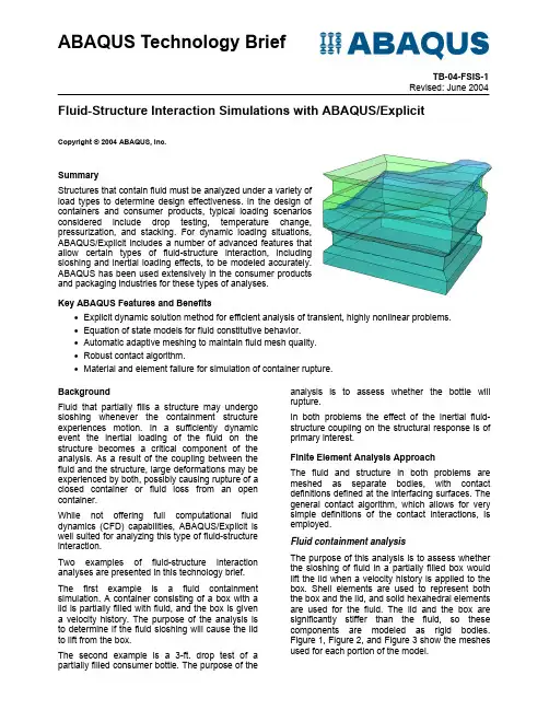
技术简介-ABAQUS显式的流固耦合仿真
ABAQUS Technology BriefTB-04-FSIS-1 Revised: June 2004Fluid-Structure Interaction Simulations with ABAQUS/ExplicitCopyright © 2004 ABAQUS, Inc.SummaryStructures that contain fluid must be analyzed under a variety of load types to determine design effectiveness. In the design of containers and consumer products, typical loading scenarios considered include drop testing, temperature change, pressurization, and stacking. For dynamic loading situations, ABAQUS/Explicit includes a number of advanced features that allow certain types of fluid-structure interaction, including sloshing and inertial loading effects, to be modeled accurately. ABAQUS has been used extensively in the consumer products and packaging industries for these types of analyses.Key ABAQUS Features and Benefits• Explicit dynamic solution method for efficient analysis of transient, highly nonlinear problems. • Equation of state models for fluid constitutive behavior. • Automatic adaptive meshing to maintain fluid mesh quality. • Robust contact algorithm. • Material and element failure for simulation of container rupture.BackgroundFluid that partially fills a structure may undergo sloshing whenever the containment structure experiences motion. In a sufficiently dynamic event the inertial loading of the fluid on the structure becomes a critical component of the analysis. As a result of the coupling between the fluid and the structure, large deformations may be experienced by both, possibly causing rupture of a closed container or fluid loss from an open container.While not offering full computational fluid dynamics (CFD) capabilities, ABAQUS/Explicit is well suited for analyzing this type of fluid-structure interaction.Two examples of fluid-structure interaction analyses are presented in this technology brief.The first example is a fluid containment simulation. A container consisting of a box with a lid is partially filled with fluid, and the box is given a velocity history. The purpose of the analysis is to determine if the fluid sloshing will cause the lid to lift from the box.The second example is a 3-ft. drop test of a partially filled consumer bottle. The purpose of theanalysis is to assess whether the bottle will rupture.In both problems the effect of the inertial fluidstructure coupling on the structural response is of primary interest.Finite Element Analysis ApproachThe fluid and structure in both problems are meshed as separate bodies, with contact definitions defined at the interfacing surfaces. The general contact algorithm, which allows for very simple definitions of the contact interactions, is employed.Fluid containment analysisThe purpose of this analysis is to assess whether the sloshing of fluid in a partially filled box would lift the lid when a velocity history is applied to the box. Shell elements are used to represent both the box and the lid, and solid hexahedral elements are used for the fluid. The lid and the box are significantly stiffer than the fluid, so these components are modeled as rigid bodies. Figure 1, Figure 2, and Figure 3 show the meshes used for each portion of the model.Figure 1: Rigid element mesh for the lid. Figure 2: Solid element mesh for the fluid.The box is constrained to remain on the horizontal plane throughout the analysis; that is, it is not allowed to rotate in space or to lift from the ground. Gravity loads are applied to the lid and to the fluid; and a sinusoidal, time-varying velocity is applied to the box. The velocity history is such that the box moves only in the horizontal plane; no vertical motion has been prescribed.The lid simply sits on the box; therefore, an airtight seal is not assumed at this interface. Consequently, there is no gas pressure in the space above the fluid. If the effect of a gas were to be included in the analysis, the following modeling approaches could be taken:• The gas could be modeled with solid elements (using an equation of state material model) and a contact interface between the fluid and the gas.• A surface-based hydrostatic fluid cavity could be defined for the gas.• A simple surface pressure load could be applied to the free surface of the fluid.Bottle drop analysisThe purpose of this analysis is to determine the integrity of a fluid-filled bottle when dropped from a height of 3 ft. Shell elements are used to represent the bottle, and solid hexahedral elements are used for the fluid. A single rigid element is used to model the floor. The undeformed model is shown in Figure 4.Figure 3: Rigid element mesh for the box.Contact is defined between the lid and the box and between the fluid and the entire container. No attachment has been defined between the lid and the box.ABAQUS has a number of contact algorithms; the general contact capability is the easiest to use and the most comprehensive. An advantage of the general contact algorithm is its ability to include the “edge-to-edge” contact at the top of the box in the contact definition. With edge-toedge contact, geometric feature edges, perimeter edges of shell and solid elements, and segments of beam and truss elements can be included in the contact domain. This feature allows contact interactions that cannot be detected as penetrations of nodes into faces to be enforced.Figure 4: Undeformed bottle, fluid, and rigid floor.Contact is defined between the bottle and the fluid and between the bottle and the floor. Gravity loads are applied to both the fluid and the container. The initial conditions of the bottle are consistent with a drop of 3 ft. The bottle is positioned slightly above the point of contact, and the fluid and the container are given an initial velocity of 168 in/s. The rigid floor is fully constrained.2The elastic-plastic constitutive properties of the bottle are those of high-density polyethylene (HDPE). A failure model is included for the HDPE, based on the tensile hydrostatic pressure stress in the elements. This failure model allows elements to be deleted from the mesh once failure has been detected. The general contact algorithm will automatically eliminate failed elements from the contact domain and update contact surfaces so that the resulting surface lies on elements that have not failed; surface erosion is a key capability in modeling the contact as the fluid sloshes out of a broken container. The base of the bottle is thicker than the walls, making the material in this region slightly more resistant to failure. This region is shown in red in Figure 5.Figure 5: Regions of different thicknesses in the bottle.The effect of any gas pressure in the bottle has been ignored. In this case the size of the enclosed gas cavity is small compared to the fluid, so the effect of the gas has been assumed negligible. The additional features common to both models are discussed below.Equation of state material model In both examples the fluid is considered as incompressible and inviscid. An equation of state material model is typically used for such applications and is chosen here. The equation of state determines the volumetric strength of a hydrodynamic material and specifies the pressure in the material as a function of density and internal energy. With this approach the deviatoric strength of the material is considered separately and can be included if viscous behavior is needed.Section properties of the fluid elements ABAQUS/Explicit offers alternative kinematic formulations for solid hexahedral elements: when appropriate for the analysis, choosing a nondefault formulation can significantly reduce computational expense. For the elementsrepresenting the fluid in the present simulations, an orthogonal formulation is chosen. This formulation provides a good balance between computational speed and accuracy. If the objective of the analyses was to determine the shape of the fluid free surface with the highest possible accuracy, the default kinematic formulation would be appropriate. However, because the inertial coupling of the fluid and structure is of primary importance, a less computationally expensive formulation can be used.Automatic adaptive meshing for the fluid Automatic adaptive meshing in ABAQUS/Explicit allows it to maintain high-quality element shapes as the fluid undergoes large deformation during sloshing. While a regular Lagrangian approach could be used to model the fluid, the elements would become very distorted after a short period of time. Adaptive meshing maintains well-shaped elements, allowing for a longer simulation time by periodically adjusting the element shapes in the fluid domain. Initially regular, relatively coarse meshes of hexahedral elements are used for the fluid. A single adaptive mesh domain that incorporates the entire fluid region is defined. In the bottle drop example a graded smoothing objective is used so that the initial mesh gradation of the water is preserved approximately while continuous adaptive meshing is performed. In addition, the default curvature refinement weighting is increased, causing the adaptive meshing algorithm to retain more elements in areas of high concave curvature.Analysis Results and Discussion Some representative results from the analyses are presented.Fluid containment analysis Figure 6–Figure 9 display the deformed shape of the fluid at several points of the analysis.Figure 6: Deformed shape after 0.12 seconds.3No restraint mechanism is applied to the lid; it is simply placed on the box. Since the lid is modeled as rigid, the history of the vertical displacement of the center of the lid (Figure 10) clearly shows that the sloshing induced in the fluid will cause the lid to separate from the box.Figure 7: Deformed shape after 0.375 seconds.Figure 10: History of vertical displacement of the lid center.Bottle drop analysisThe deformation and damage sustained by the bottle are shown in Figure 11–Figure 15.Figure 8: Deformed shape after 0.6 seconds.Figure 11: Deformed shape after 6.3 milliseconds.Figure 9: Deformed shape after 0.877 seconds.The deformed shape plots show the large deformations achieved by the fluid as the box moves. The automatic adaptive meshing capability in ABAQUS/Explicit maintains well shaped elements in the fluid, allowing the fluid to achieve high levels of deformation.Figure 12: Deformed shape after 10.8 milliseconds.4Figure 13: Deformed shape after 12.6 milliseconds.Figure 15: Deformed shape after 18 milliseconds.The deformed shape plots clearly show the buckling response of the bottle on impact and the instant of rupture (the failed elements have been removed from the plots). The tensile failure material model produces an output variable that indicates whether failure has occurred for each element, and the Visualization module in ABAQUS/CAE can remove the failed elements from the display. As the failure propagates, it can be seen that the tear travels down the corner of the bottle and turns along the interface between the thicker base section and the thinner bottle wall.Figure 14: Deformed shape after 14.4 milliseconds.ConclusionsAs demonstrated in the above analyses, ABAQUS/Explicit can be used to incorporate the effects of sloshing-type fluid-structure interaction into dynamic analyses. While it is generally not possible in ABAQUS/Explicit to model complex fluid flow behaviors or phenomena such as freesurface interactions and splashing, inclusion of the inertial loading caused by the fluid deformation allows for a more complete simulation capability.ABAQUS ReferencesFor additional information on the ABAQUS capabilities referred to in this brief, see the following ABAQUS Version 6.4 documentation references:• Analysis User’s Manual- “Explicit dynamic analysis,” Section 6.3.3 - “Adaptive meshing,” Section 7.16 - “Equation of state,” Section 10.9.1• Example Problems Manual- “Cask drop with foam impact limiter,” Section 2.1.12 - “Water sloshing in a baffled tank,” Section 2.1.14• Benchmarks Manual- “Water sloshing in a pitching tank,” Section 1.11.75。
滚筒洗衣机ABAQUS流固耦合实例分析(步骤)
例子的来源是Abaqus CLE的官方教程,可是写的太粗线条,我还是搞了两天才做出了这个例子。
其实就是个滚筒洗衣机带着洗衣机里的水一起转的问题。
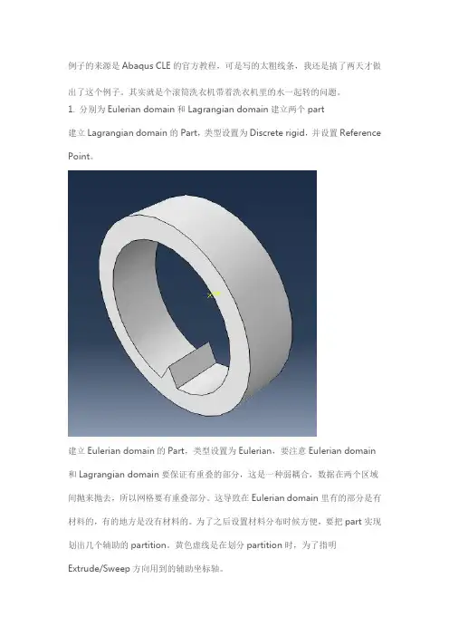
1. 分别为Eulerian domain和Lagrangian domain建立两个part建立Lagrangian domain的Part,类型设置为Discrete rigid,并设置Reference Point。
建立Eulerian domain的Part,类型设置为Eulerian,要注意Eulerian domain 和Lagrangian domain要保证有重叠的部分,这是一种弱耦合,数据在两个区域间抛来抛去,所以网格要有重叠部分。
这导致在Eulerian domain里有的部分是有材料的,有的地方是没有材料的。
为了之后设置材料分布时候方便,要把part实现划出几个辅助的partition。
黄色虚线是在划分partition时,为了指明Extrude/Sweep方向用到的辅助坐标轴。
2. 定义水的材料属性选择状态方程模型EOS中Us-Up,设置声速c0=1483m/s;密度为1000kg/m3;粘度为0.001kg/ms。
并把截面属性赋给Eulerian domain。
3. 把两个Part组装起来4. 新建一个Step-15. 为Eulerian domain和Lagrangian domain划分网格6. 设置接触新建一个Contact Property ,因为不是普通的面和面的接触,水中的任何的一个部分可能在流动区域里的任何一个地方和Lagrangian domain接触,设置Tangential Behavior为Rough,赋给水和洗衣机之间的关系。
新建一个Interaction,把刚才的Contact Property赋给它。
更重要的是设置接触的两个Surface。
其中一个Surface是Lagrangian domain 部分的内侧面,为Geometry类型,另一个Surface是Eulerian domain的全部网格,为Mesh类型。
abaqus声固耦合方法

abaqus声固耦合方法
Abaqus是一种常用的有限元分析软件,它可以用于解决声学和
固体力学问题。
声固耦合是指声学问题和固体力学问题之间的耦合
关系,也就是声波对固体的影响或者固体对声波的影响。
在Abaqus 中,可以通过声固耦合方法来模拟这种耦合关系。
在Abaqus中,声固耦合分析通常涉及到以下几个方面:
1. 声学模型,首先需要建立声学模型,包括声源、声波传播介
质和接收器等。
在Abaqus中可以使用声学元素来建立声学模型,比
如声压元素和声速元素。
2. 固体力学模型,同时需要建立固体力学模型,包括受力结构、材料性质等。
可以使用Abaqus中的固体单元来建立固体力学模型。
3. 耦合边界条件,在声固耦合分析中,需要定义声学模型和固
体力学模型之间的耦合边界条件,比如固体表面的声压加载或者固
体的振动对声波的影响。
4. 求解耦合问题,最后需要进行耦合问题的求解,Abaqus提
供了耦合分析的功能来解决声固耦合问题,可以通过设置合适的分析步骤和求解器来完成声固耦合分析。
总的来说,在Abaqus中进行声固耦合分析需要建立声学模型、固体力学模型,定义耦合边界条件并进行耦合问题的求解。
通过合理的建模和分析设置,可以模拟声波对固体的影响以及固体对声波的影响,从而完成声固耦合分析。
希望这个回答可以帮助你理解在Abaqus中进行声固耦合分析的方法。
ABAQUS流固耦合

当只进行渗流计算时:1.由于Abaqus中缺乏非耦合的孔压单元,这时可采用耦合单元,但要约束住所有位移的自由度。
2.渗流材料参数选择。
在CAE中都是在(Material-creat-other-pore fluid)选项中。
1)Gel:定义凝胶微粒吸湿膨胀的发育过程,这在一般的岩土分析中应用不多。
2)Moisture swelling:定义由于吸湿饱和所引起的固体骨架体积膨胀(或负吸力引起的骨架收缩)。
3)(3)Permeability:定义饱和介质的渗透系数,该渗透系数可以在type选项中定义为各向同性、正交各向异性和各向异性,并且可以根据Void Ratio定义为孔隙比的函数。
在Suboptions中选择Saturation Dependent 参数来指定与饱和度相关性系数ks(s),缺省设置为ks=s3,而非饱和介质渗透系数k’=ksk 选择Velocity dependence参数可以激活Forchheimer定律,缺省的是Darcy定律4)Pore Fluid Expansion:定义固体颗粒与流体体积热变化效应。
5)Porous Bulk Moduli:定义固体颗粒与流体体积模量。
6)Sorption:定义负孔隙压力与饱和度之间的相关性。
当type=Absorption时,定义吸湿曲线,type=Exsorption时定义排水曲线。
3、载荷及边界条件1)通过(Load-creat-step-fluid-surface pore fluid)选项定义沿着单元表面的外法线方向的渗流速度vn,当考虑降雨影响时可采用此载荷2)边界条件(Boundary condition-creat-other-pore pressure)选项定义孔压边界条件,此时要先假定浸润面的位置,然后定义浸润面上的孔压为零,Abaqus会在后续的分析计算中自动计算出浸润面的位置。
Abaqus默认的是不透水边界。
3)当渗流自由面遇到临空的自由排水面时,需要定义一个特殊的边界条件。
abaqus FSI流固耦合教程

适用范围
2 abaqus流固耦合简介
精品课件
2 abaqus流固耦合简介
不适用的范围 震动噪声 利用杆、梁、桁架、线缆建立的模型 喷射成形、铸造、超塑性成形 破裂、渗透分析
精品课件
2 abaqus流固耦合简介
2.2操作流程
精品课件
2 abaqus流固耦合简介
(1)定义流体介质属性
精品课件
精品课件
4、热流耦合操作与实例
1、建立几何模型 PCB板尺寸 7.8X11.6X0.16 cm 芯片尺寸 3X3X0.7 cm 发热块尺寸 1.8X1.8X0.3cm 核心尺寸 0.75X0.75X0.2cm 空气尺寸 27.8X20X12.56 cm
精品课件
4、热流耦合操作与实例
• 单元类型DC3D8 • 初始温度293K • 体热通量50mW/s/mm3 • 瞬态热传递分析步,初始增量0.01s;CFD分析;总仿真时
精品课件
2 abaqus流固耦合简介
(4)定义边界和载荷
精品课件
2 abaqus流固耦合简介
精品课件
2 abaqus流固耦合简介
精品课件
2 abaqus流固耦合简介
精品课件
2 abaqus流固耦合简介
精品课件
2 abaqus流固耦合简介
精品课件
2 abaqus流固耦合简介
精品课件
2 abaqus流固耦合简介
精品课件
3、流固耦合操作与实例
润滑油简化为不可压缩、均匀介质 质量864Kg/m3 动力粘度4.33cp 比定压热容2063J/(Kg.K) 入口速度1.93m/s
单位mm,圆角R100 精品课件
3、流固耦合操作与实例
流固耦合分析(FSI)理论详解

流固耦合分析(FSI)流固耦合分析(FSI)是涉及流体和固体之间相互作用的问题研究,其理论包括了几个主要方面:流体力学、固体力学、耦合边界条件、求解器等。
以下是流固耦合分析的详细理论讲解,带有相关公式和尽量详细的说明。
一、流体力学1. 守恒定律质量守恒定律:$$ \frac{\partial \rho}{\partial t} + \nabla \cdot (\rho \mathbf{u}) = 0 $$动量守恒定律:$$ \rho \frac{\partial \mathbf{u}}{\partial t} + \rho (\mathbf{u} \cdot \nabla) \mathbf{u} = \nabla \cdot \tau + \mathbf{f} $$其中,$\rho$是流体密度,$\mathbf{u}$是流体速度,$\tau$是应力张量,$\mathbf{f}$是体力。
2. 纳维-斯托克斯方程$$ \rho \frac{\partial \mathbf{u}}{\partial t} + \rho (\mathbf{u} \cdot \nabla) \mathbf{u} = \nabla \cdot (-p\mathbf{I} + \tau) + \mathbf{f} $$其中,$p$是静压力,$\mathbf{I}$是单位张量。
3. 边界条件(1)速度边界条件:$\mathbf{u} = \mathbf{u}_b$,其中$\mathbf{u}_b$是边界上的速度。
(2)压力边界条件:$p = p_b$,其中$p_b$是边界上的压力。
4. 流体力学求解器常用的流体力学求解器有OpenFOAM、ANSYS Fluent等。
二、固体力学1. 力学基本方程$$ \tau = \sigma\cdot \mathbf{n} $$其中,$\tau$是表面上的接触力,$\sigma$是固体的应力张量,$\mathbf{n}$是表面的单位法向量。
流固耦合过程_教程
湖南大学先进动力流固耦合过程(仅耦合热边界)准备软件:¾AVL-FIRE¾Hypermesh(用于划分和处理网格)¾ABAQUS(熟悉inp文件结构和语句)¾MSC-Patran湖南大学先进动力以AVL-FIRE安装目录下面简单例子为例,位于以下目录:D(安装盘符):\AVL\FIRE\v(版本号)\exam湖南大学先进动力第一步:CFD计算所有设置与例子中保持一致湖南大学先进动力第一步计算CFD的时候,不需要选上Mesh FEM format,只需指定输出Frequency即可。
湖南大学先进动力第一步计算完之后会产生一个htcc 文件,如下图:湖南大学先进动力第二步:耦合面网格及固体网格获取为了便于统一坐标位置和热边界插值,不用例子中的FEM 网格。
FEM 网格将从CFD 网格(cyl.flm )中“抽取”,如下图,在Fire 中导出.nas 格式文件。
湖南大学先进动力在hypermesh中TOOl>faces 板块中把流体网格的外表面抽取,然后删除两端面的面网格选择全部网格(displayed)即可湖南大学先进动力通过3D>elem offset 来获得实体网格湖南大学先进动力第三步:映射(mapping )热边界条件上一步得到的面网格导出为.nas 文件(如sur_mesh_for_mapping.nas )FIRE 中FEM Interface中设置如下两图湖南大学先进动力保存之后,Start ,next 直到如图所示界面,输入-fem –mode=mapping湖南大学先进动力第四步:查看热边界结果(这一步不是必需的,为了Mapping之后会产生一个包含热边界的inp文件,用于后续的固体温度场计算。
湖南大学先进动力映射距离与用例子比较(用三角形面单元)湖南大学先进动力第五步:在MSC-Patran 中做MPC注意:这里的面网格节点号和单元号要与前面用来mapping 的面网格对应上,可以在patran 或者hypermesh 中通过renumber 来实现,固体网格最好也把节点号和单元号renumber ,记下所有的节点号和单元号,以备后用。
Abaqus流固耦合仿真方法大全,总有你的菜,哪怕是佛系
Abaqus流固耦合仿真⽅法⼤全,总有你的菜,哪怕是佛系对于⼀般的流固耦合问题,Abaqus提供的仿真⽅法多种多样,最常⽤的三⼤类是:1.协同求解需要不同求解器之间进⾏通信:a.使⽤SIMULIA 协同仿真引擎b.使⽤多场耦合分析⼯具MpCCIc.使⽤Abaqus的ZAERO接⼝程序2.CEL3.SPH⽽特殊流固耦合问题,⽐如渗流(Seepage分析)、湿模态(可⽤Acoustic单元)、流体腔(Fluid Cavity)等,Abaqus也都有对应的分析⼿段。
最近问到的流固耦合问题⽐较多,这期⽂章就介绍⼀下Abaqus常⽤的三⼤类流固耦合分析⽅法。
1.协同求解a.使⽤SIMULIA协同仿真引擎⾸先要有两个model,⼀个CFD,⼀个Structure,定义耦合界⾯,并分别创建两个作业;然后通过SIMULIA协同仿真引擎引⽤两个model的作业,创建⼀个协同仿真;最后提交协同仿真任务,在模型树中可调出两个协同分析作业的监控。
Abaqus/CFD特点:能够进⾏不可压缩流体(通常认为是液体或者密度变化相对较⼩的⽓体,0≤Ma≤0.1~0.3)动⼒学分析,可以是层流或湍流(4种湍流模型)、稳态或瞬态(能够使⽤ALE变形⽹格)。
流体参数:密度、粘度、初始速度、等压⽐热容、热膨胀系数。
⼯程应⽤领域:⼤⽓扩散、汽车⽓动设计、⽣物医药、⾷品加⼯、电器冷却、模具填充等。
6.10版引⼊CFD求解器,2017版取消,因此该⽅法只能在Abaqus有限版本内使⽤:SIMULIA Co-simulation Engine简介:达索SIMULIA的多场耦合求解平台,内置于Abaqus Job模块,功能强⼤,可以⽤于耦合Abaqus不同求解器或第三⽅求解器,⽐如单独在Abaqus内可以做到:①流固耦合将⼀个Abaqus/Standard或Abaqus/Explicit分析过程与⼀个Abaqus/CFD分析过程进⾏协同;②共轭热传导将⼀个Abaqus/Standard分析过程与⼀个Abaqus/CFD分析过程进⾏协同;③电磁-热或电磁-⼒学耦合将两个Abaqus/Standard分析过程进⾏协同;④隐式瞬态分析和显式动态分析之间耦合将⼀个Abaqus/Standard分析过程与⼀个Abaqus/Explicit分析过程进⾏协同。
[P]ABAQUS流固耦合之 增量步参数设置
[P]ABAQUS流固耦合之增量步参数设置----e0a22f3a-6ea4-11ec-a67b-7cb59b590d7d[p]abaqus流固耦合之--增量步参数设置1.ABAQUS流固耦合分析步骤参数设置(1)abaqus流固耦合分析步参数设置-basicTimeperiod是分析步骤的总时间。
例如,如果图中设置为86400s(该单位与建模时设置的系统单位一致,以下时间单位默认为秒),则认为分析步骤在86400s内完成,即24小时。
(2)editstep―incrementation,增量步的设置通常,类型选择自动选项,即,系统根据计算速度和收敛程度自动调整增量步长(fixed是一个固定的增量步骤,如果每一步设置8640,将执行10步,最终总时间为86400。
不建议使用此选项,当模型复杂时,很容易导致不收敛)maximumnumberofincrements,默认为100,模型复杂不易收敛时,可将其调大,即最大迭代次数增加(通常设置1000即足够)。
初始,初始增量步长,通常设置为时间周期的0.1~0.01倍。
如果模型具有良好的收敛性,系统将通过自动功能自动增加增量步长,以加快计算速度。
max.porepressurechangeperincrement,允许每步最大增量,该选项建议调大,例如本模型初始孔压最大值为6e5pa,则该选项可设定大于e5的数量级(设置过小,如e-5,则每步允许增量步太小,反复迭代次数过多易导致不收敛),EndStep当无法设置ExpressureChangeRateIsLessThan时,即其计算被视为最终终止。
(3)other其他选项求解非线性模型时,通常检查不对称性。
以下为网络帖子,其所遇到问题正是由于增量步设置导致(尤其最大允许增量步的设置),供参考。
2.职位1[流固耦合]abaqus流固耦合进行瞬态分析时,设定的utol是什么意义?例如,最近的模拟是注水试验过程。
Abaqus热流固耦合——围绕圆柱形热源进行固结
Abaqus热流固耦合——围绕圆柱形热源进行固结翻译抖音号abaquser,qq443941211这个问题提出了在圆柱形热源周围饱和土壤中固结的解决方案。
布克和萨维维杜(Booker and Savvidou,1985)对该问题进行了研究,它代表了埋在饱和土壤中的放射性废物罐问题的理想化。
由于来自罐的热辐射而发生的温度变化导致孔隙水的膨胀量大于土壤中的孔隙,导致热源周围的孔隙压力增加。
产生的孔隙压力梯度将孔隙流体驱离热源,导致孔隙压力随时间消散。
Booker和Savvidou开发了针对点热源深埋在饱和土壤中的基本问题的分析解决方案。
随后,他们使用该分析解决方案得出了圆柱热源周围固结问题的近似解决方案。
该问题为Abaqus中的耦合热固结能力提供了验证。
饱和土壤的分析需要耦合应力-扩散方程的解,Abaqus中使用的公式在《Abaqus理论指南》第2.8节“多孔介质分析”中有详细描述。
热固结能力还可以与应力扩散方程完全耦合地求解传热方程(同时考虑传导和对流效应),从而模拟孔隙压力对孔隙流体和管道中温度场的影响。
土壤,反之亦然。
定义几何形状和材料特性的参数的数值是基于Lewis和Schrefler(2000)对这个问题进行的参数研究中给出的细节。
问题描述问题设置如图1.15.7-1所示。
半径为0.1604m,高度为2.5m的圆柱形热源被埋在半径和高度均等于10m的圆柱形土壤中。
实际上,土壤的圆柱形体积代表了围绕热源的无限介质。
重力被忽略了。
由于边界条件(下面将详细讨论),问题基本上是一维的,唯一的梯度是在径向上。
分析的目的是预测整个土壤质量,特别是热源附近的孔隙压力和温度随时间的变化。
几何和模型利用垂直方向的对称性,仅对问题的一半进行建模。
使用三维和轴对称的温度-孔压力元件均可解决此问题。
为了呈现结果,选择了三维元素类型C3D8RPT。
三维分析和轴对称分析均使用基本三维8节点或轴对称4节点元素以及修饰的四面体元素的不同变体(例如,积分和混合)进行。