MATLAB编程求解二维泊松方程doc资料
matlab二维有限元编程

matlab二维有限元编程Matlab是一种常用的数学软件,广泛应用于科学计算和工程领域。
在有限元分析中,Matlab可以用来进行二维有限元编程,实现对复杂结构的力学行为进行模拟和分析。
本文将介绍如何使用Matlab进行二维有限元编程,并给出一些实例来说明其应用。
二维有限元编程是一种将连续的物理问题离散化处理的方法,通过将连续问题转化为离散的节点和单元来进行分析。
在Matlab中,我们可以使用网格生成工具来创建二维网格,然后将其转化为节点和单元的数据结构。
节点表示问题的离散点,而单元则表示节点之间的连接关系。
在二维有限元编程中,我们通常需要定义材料的性质、载荷条件和边界条件。
材料的性质可以包括弹性模量和泊松比等。
载荷条件可以包括集中力、分布力和压力等。
边界条件可以包括固支、自由支承和位移约束等。
在Matlab中,我们可以通过定义相应的矩阵和向量来表示这些条件。
接下来,我们需要根据节点和单元的数据结构建立刚度矩阵和载荷向量。
刚度矩阵描述了节点之间的刚度关系,而载荷向量描述了节点上的外力作用。
在Matlab中,我们可以使用循环和矩阵运算来建立这些矩阵和向量。
然后,我们可以通过求解线性方程组的方法来计算节点的位移和应力。
我们可以根据节点的位移和应力来进行结果的后处理。
后处理可以包括绘制位移和应力云图、计算节点和单元的应变能和应力分布等。
在Matlab中,我们可以使用绘图函数和计算函数来实现这些后处理操作。
下面是一个简单的例子来说明如何使用Matlab进行二维有限元编程。
假设我们要分析一个弹性材料的悬臂梁,在梁的一端施加一个集中力。
首先,我们需要定义材料的性质、载荷条件和边界条件。
然后,我们可以使用网格生成工具创建二维网格,并将其转化为节点和单元的数据结构。
接下来,我们可以建立刚度矩阵和载荷向量,并求解线性方程组得到节点的位移。
最后,我们可以进行结果的后处理,如绘制位移和应力云图。
Matlab提供了强大的工具和函数来进行二维有限元编程。
有限元法求解二维Poisson方程的MATLAB实现
(x,y) e 9 0 ,
其中
— ax ay
e i 2(/3), 为 i?2 中的
有界凸区域,区 域 / 3 = { ( * ,;K) U2 + y2 < l }.
1 二 维 P oisson方程的有限元法
l .i 有限元方法的基本原理和步骤 有限元法是基于变分原理和剖分技术的一种数
值计算方法,把微分方法的定解问题转化为求解一
摘 要 :文 章 讨 论 了 圆 形 区 域 上 的 三 角 形 单 元 剖 分 、有 限 元 空 间 ,通 过 变 分 形 式 离 散 得 到 有 限 元 方 程 .用 M A T L A B 编程求得数值解,并进行了误差分析. 关 键 词 :Poisson方 程 ;有限元方法;M A T L A B 编 程 ;三角形单元剖分
U e l f +2( n , R m).
定理[7]1 (有 限 元 近 似 解 的 炉 模 估 计 )假设 满足引理的条件,则 对 V f/ E 妒+1(/3,i T ) ,存在与 A 无 关 的常数C , 使得
W u - u . w, ^ chk \ u \ M
定理[7]2 (有 限 元 近 似 解 的 i 2 模 估 计 )假设
1
0
0
0
2
3
0
0
細 !1[8]:
4
560ຫໍສະໝຸດ 中 图 分 类 号 :0241.8
文 献 标 识 码 :A
文章编号:1009 - 4 9 7 0 ( 2 0 1 8 ) 0 5 - 0015 - 04
0 引言
热 学 、流 体 力 学 、电 磁 学 、声 学 等 学 科 中 的 相
关 过 程 ,都 可 以 用 椭 圆 型 方 程 来 描 述 .最 为 典 型 的
利用有限差分和MATLAB矩阵运算直接求解二维泊松方程
以求解 大型 线性 方程 组 。 关 键词 :半 导体 ; 泊松方 程 ;有 限差分 法 ;MA L T AB
中图分 类号 :T 0 N3 1 文献标 识码 :A 文章编 号 : 10 —8 12 1)40 1 —4 0 18 9 (0 00 —2 30
Di e tSo uto fTwo di e i na is n Eq to r c l ino - m nso l Po s o ua i n
1 二 维 泊 松 方 程 在 正 方 形 网 格 节 点 上 的 有 限 差 分
Abs r c :Ba e n fn t if r n ep n i l s a e o ut e i n i i i e n o a s reso ic ee n de ta t s d o ied fe e c r c p e , f rs l i r g o sd v d d i t e i fd s r t o s i i t on
p o r m mi g. rga n
Ke r : s mi on u t r Po s o qu ton, fn t i e e c t od, M ATLAB y wo ds e c d co , i s n e ai i ied f r n eme h
摹
半 导 体 器 件 模 拟 中 的静 电场 问题 可 归 结 为 在 给 定 电荷 分布 和边 界条 件 下求 解泊 松 方程…。和 薛定 谔
(完整版)基于MATLAB的泊松分布的仿真
(完整版)基于MATLAB的泊松分布的仿真泊松过程样本轨道的MATLAB 仿真⼀、 Poisson Process 定义若有⼀个随机过程{:0}t N N t =≥是参数为λ>0的Poisson 过程,它满⾜下列条件: 1、0N = 0;2、对任意的时间指标0s t ≤<,增量()()t s N N t s ω-ωλ(-)服从参数为泊松分布。
3、对任意的⾃然数n ≥2和任意的时间指标0120n t t t t =<<12110,,n n t t t t t t N N N N N N --?,--是相互独⽴的随机变量。
⼆、从泊松过程的定义可知1、泊松过程具有平稳独⽴增量性。
2、时间指标集合为[ 0 , +∞],状态空间为*S=N 。
3、泊松过程是⼀个连续时间离散状态的随机过程。
三、MATLAB 仿真泊松过程的思想1、若定义i T 为泊松过程的到达时间,1,n n n T T n τ=+-∈N 为到达时间间隔。
那么泊松过程N 的到达时间间隔{:}n n N τ∈是相互独⽴且同服从于参数为λ的指数分布。
2、若U 是服从于[0,1]的均匀分布,则1()E Ln U =-λ服从于参数为λ的指数分布。
利⽤随机变量分布函数的定义很容易证明这条性质。
3、由于1、和2、中的条件成⽴,现在我们考虑11[()]n n n T T Ln U n τ=+=--λ那么就可以推出11[()]n n T T Ln U n +=-λ在MATLAB 中我们可以⽤rand(1,K)产⽣⼀个具有K 个值的随机序列,它们在[0,1]上服从于均匀分布,利⽤上式计算出 n T ,在每⼀个到达时间 n T 处,N 的值从n-1变成n 。
⽤plot 函数就可以将样本轨道画出了。
四、MATLAB 程序1、⾸先我们建⽴⼀个poisson 函数,即poisson.m:function poisson(m)%This function can help us to simulate poisson processes. %If you give m a integer like 1 2 3 and so on ,then you will get %a figure to illustrate the m sample traces of the process. %rand('state',0); %复位伪随机序列发⽣器为0状态 K=10; %设置计数值为10%m=6; %设置样本个数color=char('r+','b+','g+','m+','y+','c+'); %不同的轨道采⽤不同的颜⾊表⽰lambda=1; %设置到达速率为1for n=1:mu=rand(1,K); %产⽣服从均匀分布的序列T=zeros(1,K+1); %长⽣K+1维随机时间全零向量k=zeros(1,K+1); %产⽣K+1维随机变量全零向量for j=1:Kk(j+1)=j;T(j+1)=T(j)-log(u(j))/lambda; %计算到达时间endfor i=1:Kplot([T(i):0.001:T(i+1)],[k(i):k(i)],color(n,[1,2])); hold on;endend2、下⾯我们在命令窗⼝键⼊以下命令:clear;poisson(1);就可以得到⼀条样本轨道,如下所⽰:键⼊poisson(2),得到的图如下:键⼊poisson(3),得到的图如下:键⼊poisson(4),仿真结果:键⼊poisson(5),仿真结果:键⼊poisson1(6),仿真结果:。
matlaB程序的有限元法解泊松方程.doc

基于matlaB 编程的有限元法一、待求问题:泛定方程:2=x ϕ-∇边界条件:以(0,-1),(0,1),(1,0)为顶点的三角形区域边界上=0ϕ二、编程思路及方法1、给节点和三角形单元编号,并设定节点坐标画出以(0,-1),(0,1),(1,0)为顶点的三角形区域figure1由于积分区域规则,故采用特殊剖分单元,将区域沿水平竖直方向分等份,此时所有单元都是等腰直角三角形,剖分单元个数由自己输入,但竖直方向份数(用Jmax 表示)必须是水平方向份数(Imax )的两倍,所以用户只需输入水平方向的份数Imax 。
采用上述剖分方法,节点位置也比较规则。
然后利用循环从区域内部(非边界)的节点开始编号,格式为NN(i,j)=n1,i ,j 分别表示节点所在列数与行数,并将节点坐标存入相应矩阵X(n1),Y(n1)。
由于区域上下两部分形状不同因此,分两个循环分别编号赋值,然后再对边界节点编号赋值。
然后再每个单元的节点进行局部编号,由于求解区域和剖分单元的特殊性,分别对内部节点对应左上角正方形的两个三角形单元,上左,左上,下斜边界节点要对应三个单元,上左,左上,左下,右顶点的左下、左上,右上边界的左上,分别编号以保证覆盖整个区域。
2、求解泊松方程首先一次获得每个单元节点的整体编号,然后根据其坐标求出每个三角形单元的面积。
利用有限元方法的原理,分别求出系数矩阵和右端项,并且由于边界,因此做积分时只需对场域单元积分而不必对边界单元积条件特殊,边界上=0分。
求的两个矩阵后很容易得到节点电位向量,即泊松方程的解。
3、画解函数的平面图和曲面图由节点单位向量得到,j行i列节点的电位,然后调用绘图函数imagesc(NNV)与surf(X1,Y1,NNV')分别得到解函数的平面图figure2和曲面图figure3。
4、将结果输出为文本文件输出节点编号,坐标,电位值三、计算结果1、积分区域:2、f=1,x 方向75份,y 方向150份时,解函数平面图和曲面图20406080100120140102030405060700.0050.010.0150.020.0250.0320.0050.010.0150.020.0250.03对比:当f=1时,界函数平面图20406080100120140102030405060700.010.020.030.040.050.060.073、输出文本文件由于节点多较大,列在本文最末四、结果简析由于三角形区域分布的是正电荷,因此必定电位最高点在区域中部,且沿x 轴对称,三角形边界电位最低等于零。
泊松方程 neumann 边界 matlab

在MATLAB中解决带有Neumann边界条件的泊松方程,可以使用内置的偏微分方程求解器pdepe。
以下是一个简单的示例:假设我们有一个二维的泊松方程:Δu = f并且我们有一个Neumann边界条件:grad(u) · n = g这里,n是边界的外法线向量,g是已知的Neumann边界条件。
首先,我们需要定义问题的大小和区域。
假设我们的区域是[0,1]×[0,1],我们可以使用pdepe函数来求解这个问题。
以下是一个示例代码:matlab复制代码% 定义区域和网格大小[x, y] = meshgrid(0:0.01:1, 0:0.01:1);[X, Y] = ndgrid(0:0.01:1, 0:0.01:1);[Xf,Yf] = mesh2patch(X(:),Y(:));N = length(Xf);x = reshape(Xf, size(x));y = reshape(Yf, size(y));% 定义函数f和gf = -6*pi*pi*sin(pi*x).*sin(pi*y);g = -pi*cos(pi*x).*sin(pi*y);g = g(:); % flatten the vector% 定义初值条件和边界条件u = zeros(size(x)); % 初始条件,全为0Du = zeros(size(x)); % 对u的偏导数,全为0bc = []; % 边界条件,空向量表示所有边界都是Dirichlet边界bcs = {'u','Du'}; % 边界条件的标识符,'u'表示u在边界上的值,'Du'表示u的偏导数在边界上的值% 求解泊松方程options = optimset('Display','off'); % 不显示求解过程[U,Fval] = pdepe(bcs,x,y,u,Du,f,bc,options);注意,这只是一个简单的示例。
二维泊松方程很基础详细的求解过程
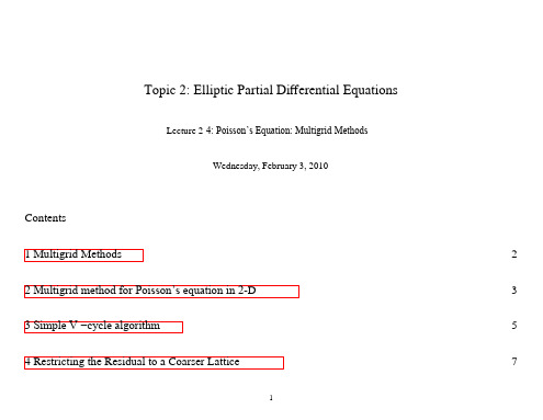
Topic 2: Elliptic Partial Differential EquationsLecture 2-4: Poisson’s Equation: Multigrid MethodsWednesday, February 3, 2010Contents1 Multigrid Methods2 Multigrid method for Poisson’s equation in 2-D3 Simple V −cycle algorithm4 Restricting the Residual to a Coarser Lattice 2 35 71 MULTIGRID METHODS5 Prolongation of the Correction to the Finer Lattice6 Cell-centered and Vertex-centered Grids and Coarsenings7 Boundary points8 Restriction and Prolongation Operators9 Improvements and More Complicated Multigrid Algorithms8 8 11 11 151 Multigrid MethodsThe multigrid method provides algorithms which can be used to accelerate the rate of convergence of iterative methods, such as Jacobi or Gauss-Seidel, for solving elliptic partial differential equations.Iterative methods start with an approximate guess for the solution to the differential equation. In each iteration, the difference between the approximate solution and the exact solution is made smaller.One can analyze this difference or error into components of different wavelengths, for example by using Fourier analysis. In general the error will have components of many different wavelengths: there will beshort wavelength error components and long wavelength error components.Algorithms like Jacobi or Gauss-Seidel are local because the new value for the solution at any lattice site depends only on the value of the previous iterate at neighboring points. Such local algorithms are generally more efficient in reducing short wavelength error components.The basic idea behind multigrid methods is to reduce long wavelength error components by updating blocks of grid points. This strategy is similar to that employed by cluster algorithms in Monte Carlo simulations of the Ising model close to the phase transtion temperature where long range correlations are important. In fact, multigrid algorithms can also be combined with Monte Carlo simulations.2 Multigrid method for Poisson’s equation in 2-DWith a small change in notation, Poisson’s equation in 2-D can be written:∂ 2u ∂x2 +∂ 2u∂y2= −f (x, y) ,where the unknown solution u(x, y) is determined by the given source term f (x, y) in a closed region. Let’s consider a square domain 0 ≤ x, y ≤ 1 with homogeneous Dirichlet boundary conditions u = 0 on the perimeter of the square. The equation is discretized on a grid with L + 2 lattice points, i.e., L interior points and 2 boundary points, in the x and y directions. At any interior point, the exact solution obeysu i,j = 14u i+1,j + u i−1,j + u i,j+1 + u i,j−1 + h2f i,j .The algorithm uses a succession of lattices or grids. The number of different grids is called the number of multigrid levels . The number of interior lattice points in the x and y directions is then taken to be 2 , so that L = 2 + 2, and the lattice spacing h = 1/(L − 1). L is chosen in this manner so that the downward multigrid iteration can construct a sequence of coarser lattices with2−1→ 2−2→ . . . → 20 = 1interior points in the x and y directions.Suppose that u(x, y) is the approximate solution at any stage in the calculation, and u exact(x, y) is the exact solution which we are trying to find. The multigrid algorithm uses the following definitions:· The correctionv = u exact− uis the function which must be added to the approximate solution to give the exact solution. · The residual or defect is defined asr = 2 u + f .Notice that the correction and the residual are related by the equation2 v = 2 u exact+ f − 2 u + f = −r .This equation has exactly the same form as Poisson’s equation with v playing the role of unknown function and r playing the role of known source function!3 SIMPLE V −CYCLE ALGORITHM3 Simple V −cycle algorithmThe simplest multigrid algorithm is based on a two-grid improvement scheme. Consider two grids:· a fine grid with L = 2 + 2 points in each direction, and· a coarse grid with L = 2−1 + 2 points.We need to be able to move from one grid to another, i.e., given any function on the lattice, we need to able to· restrict the function from fine → coarse, and· prolongate or interpolate the function from coarse → fine.Given these definitions, the multigrid V −cycle can be defined recursively as follows:· If = 0 there is only one interior point, so solve exactly foru1,1 = (u0,1 + u2,1 + u1,0 + u1,2 + h2f1,1)/4 .· Otherwise, calculate the current L = 2 + 2.3 SIMPLE V −CYCLE ALGORITHM· Perform a few pre-smoothing iterations using a local algorithm such as Gauss-Seidel. The idea is to damp or reduce the short wavelength errors in the solution.· Estimate the correction v = u exact− u as follows:– Compute the residualr i,j = 1h2 [u i+1,j + u i−1,j + u i,j+1 + u i,j−1− 4u i,j] + f i,j .–Restrict the residual r → R to the coarser grid.– Set the coarser grid correction V = 0 and improve it recursively.–Prolongate the correction V → v onto the finer grid.· Correct u → u + v.· Perform a few post-smoothing Gauss-Seidel interations and return this improved u. How does this recursive algorithm scale with L? The pre-smoothing and post-smoothing Jacobi or Gauss- Seidel iterations are the most time consuming parts of the calculation. Recall that a single Jacobi or Gauss-Seidel iteration scales like O(L2). The operations must be carried out on the sequence of grids with2 → 2−1→ 2−2→ . . . → 20 = 1interior lattice points in each direction. The total number of operations is of orderL2n=0122n≤ L211 .1 − 44 RESTRICTING THE RESIDUAL TO A COARSER LATTICEThus the multigrid V −cycle scales like O(L 2), i.e., linearly with the number of lattice points N!4Restricting the Residual to a Coarser LatticeThe coarser lattice with spacing H = 2h is constructed as shown. A simple algorithm for restricting the residual to the coarser lattice is to set its value to the average of the values on the four surrounding lattice points (cell-centered coarsening):6 CELL-CENTERED AND VERTEX-CENTERED GRIDS AND COARSENINGSR I,J = 14[r i,j + r i+1,j + r i,j+1 + r i+1,j+1] , i = 2I − 1 , j = 2J − 1 .5 Prolongation of the Correction to the Finer LatticeHaving restricted the residual to the coarser lattice with spacing H = 2h, we need to solve the equation2 V = −R(x, y) ,with the initial guess V (x, y) = 0. This is done by two-grid iterationV = twoGrid(H, V, R) .The output must now be i nterpolated or prolongated to the finer lattice. The simplest procedure is to copy the value of V I,J on the coarse lattice to the 4 neighboring cell points on the finer lattice: v i,j = v i+1,j = v i,j+1 = v i+1,j+1 = V I,J , i = 2I − 1, j = 2J − 1 .6 Cell-centered and Vertex-centered Grids and CoarseningsIn the cell-centered prescription, the spatial domain is partitioned into discrete cells. Lattice points are defined at the center of each cell as shown in the figure:The coarsening operation is defined by doubling the size of a cell in each spatial dimension and placing a coarse lattice point at the center of the doubled cell.Note that the number of lattice points or cells in each dimension must be a power of 2 if the coarsening operation is to terminate with a single cell. In the figure, the finest lattice has 23 = 8 cells in each dimension, and 3 coarsening operations reduce the number of cells in each dimension23= 8 → 22= 4 → 21= 2 → 20 = 1 .Note also that with the cell-centered prescription, the spatial location of lattice sites changes with each coarsening: coarse lattice sites are spatially displaced from fine lattice sites.A vertex-centered prescription is defined by partitioning the spatial domain into discrete cells and locating the discrete lattice points at the vertices of the cel ls as shown in the figure:The coarsening operation is implemented simply by dropping every other lattice site in each spatial dimension. Note that the number of lattice points in each dimension must be one greater than a power of 2 if the coarsening operation is to reduce the number of cells to a single coarsest cell. In the example in the figure the finest lattice has 23 + 1 = 9 lattice sites in each dimension, and 2 coarsening operations reduce the number of vertices in each dimension23+ 1 = 9 → 22+ 1 = 5 → 21 + 1 = 3 .The vertex-centered prescription has the property that the spatial locations of the discretization points are not changed by the coarsening operation.8 RESTRICTION AND PROLONGATION OPERATORS7 Boundary pointsLet’s assume that the outermost perimeter points are taken to be the boundary points. The behavior of these boundary points is different in the two prescriptions:· Cell-centered Prescription: The boundary points move in space towards the center of the region at each coarsening. This implies that one has to be careful in defining the “boundary values” of the solution.· Vertex-centered Prescription: The boundary points do not move when the lattice is coarsened.This make i t easier in principle to define the boundary values.These two different behaviors of the boundary points make the vertex-centered prescription a little more convenient to use in multigrid applications. However, there is no reason why the cell-centered prescription should not work as well.8 Restriction and Prolongation OperatorsIn the multigrid method it is necessary to move functions from a fine grid to the next coarser grid (Restric- tion), and from a coarse grid to the next finer grid (Prolongation). Many prescriptions for restricting andprolongating functions have been studied. Let’s consider two of the simplest prescriptions appropriate for cell- and vertex-centered coarsening:· Cell-centered Coarsening: In this prescription, a coarse lattice point is naturally associated with 2d neighboring fine lattice points in d-dimensions.· Suppose that f (x) is a function on the fine lattice at spatial position x, and F (X ) is the corresponding function on the coarse lattice, then this diagram suggests a simple prescription for restriction and prolongation.–Restriction: Average the function values at the 4 neighboring fine lattice sites x i:F (X ) = 144i=1f (x i) .– Prolongation: Inject the value of the function at the coarse lattice site to the 4 neighboring fine lattice sites:f (x i) = F (X ) , i = 1 . . . 4· Vertex-centered Coarsening: Consider a coarse lattice point and the 9 neighboring fine lattice points shown in the figure:2 2 · In this prescription, a coarse lattice point can naturally associated (in 2-D) with · the corresponding fine lattice point, or· the four nearest neighbor fine lattice points, left, right, up, and down, or · with the four diagonally nearest fine lattice points, etc.· It is a little more complicated here to define transfer operators. The problem is that the fine lattice points are associated with more than one coarse lattice point, unlike the cell-centered case: – The single red fine lattice point in the center coincides with an unique coarse lattice point. – Each of the 4 black fine lattice points however is equidistant from two coarse lattic e points. – Each of the 4 red fine lattice points is equidistant from four coarse lattice points. · This sharing of lattice points suggests the following prescriptions:· Prolongation: use bilinear interpolation in which the value of F at a coarse grid point is copied to 9 neighboring fine -grid points with the following weights:1 1 14 2 1 1 1 1 4 1 1.4 24This matrix is called the stencil for the prolongation.8 8 9 IMPROVEMENTS AND MORE COMPLICATED MULTIGRID ALGORITHMS· Restriction: The restriction operator is taken to be the adjoint of the prolongation operator:1 1 116 1 1 16 8 1 4 1 8 161 1 16.This choice of restriction operator is called full weighting.9Improvements and More Complicated Multigrid AlgorithmsThe algorithm implemented above is the simplest multigrid scheme with a single V-cycle. Section 19.6 of Numerical Recipes discusses various ways of improving this algorithm:· One can repeat the two-grid iteration more than once. If it is repeated twice in each multigrid level one obtains a W-cycle type of algorithm.· The Full Multigrid Algorithm starts with the coarsest grid on which the equation can be solved exactly. It then proceeds to finer grids, performing one or more V -cycles at each level along the way. Numerical Recipes gives a program mglin(u,n,ncycle) which accepts the source function −f in the first argument and implements the full multigrid algorithm with = log 2(n − 1) levels, performing ncycle V-cycles at each level, and returning the solution in the array parameter u. Note that this program assumes that the number of lattice points in each dimension L is odd, which leads to vertex centered coarsening:REFERENCESREFERENCESReferences[Recipes-C19-5] W.H. Press, S.A. Teukolsky, W. Vetterling, and B.P. Flannery, “Numerical Recipes in C”,Chapter 19 §6: Multigrid Methods for Boundary Value Problems, /a/bookcpdf/c19-6.pdf.。
matlab泊松方程第二类边界

泊松方程是数学和物理学中的一个重要方程,描述了在给定边界条件下,场的分布情况。
在工程学、地理学、地球物理学以及生物学等领域都有着广泛的应用。
而在数学和科学计算软件领域,Matlab是一个强大的工具,可以用于求解泊松方程并对其进行深入的研究。
Matlab作为一款高效的科学计算软件,提供了丰富的数学工具箱,其中包括了解决偏微分方程(PDE)的工具。
泊松方程作为一种二维的偏微分方程,在Matlab中有着完善的求解方式,而第二类边界条件则是泊松方程中的一种特殊情况,值得我们深入探讨。
在处理泊松方程第二类边界条件时,我们需要明确边界条件的定义和意义。
泊松方程第二类边界条件通常是指在边界上给定了场函数的某种形式,比如通过边界上的电势来定义电场的分布。
在Matlab中,我们可以通过指定边界条件的类型和数值来求解泊松方程,进而得到不同边界条件下场的分布情况。
在求解泊松方程第二类边界条件时,我们首先需要构建二维的网格模型,并在网格上定义泊松方程的离散形式。
根据边界条件的要求,我们可以在网格的边界上指定相应的数值。
通过Matlab提供的PDE工具箱,可以很方便地对这些边界条件进行处理,并求解泊松方程得到场的分布情况。
在实际求解中,我们还需要考虑网格的精细程度、求解的精度要求以及计算效率等因素。
在Matlab中,我们可以通过调整网格的密度和使用不同的求解算法来得到更精确和高效的结果。
Matlab还提供了丰富的可视化工具,可以直观地展示泊松方程第二类边界条件下场的分布情况,使我们更好地理解并分析结果。
总结来看,Matlab作为一款强大的科学计算软件,为我们提供了丰富的工具和方法来求解并研究泊松方程第二类边界条件。
在实际应用中,我们可以通过合理地设置边界条件、调整网格密度和求解算法,得到满足精度和计算效率要求的结果。
通过对泊松方程第二类边界条件的深入研究和分析,可以更好地理解场的分布情况,为工程、物理和其他领域的问题提供有效的解决方案。