宏观经济学作业(第四版)
宏观经济学作业(必作)

宏观经济学习题(必作)第一章:1.如何理解宏观经济学的研究对象?2.简述宏观经济学的学科体系。
3.试说明宏观经济学是怎样运用总量分析方法的。
4.古典经济学家有哪些主要的宏观经济观点?5.新古典经济学形成了哪些重要的宏观经济思想?6.凯恩斯革命的主要内容是什么?7.凯恩斯主义宏观经济理论的逐步完善主要体现在哪些方面?8.宏观经济学进一步发展呈现出哪些重要趋势?第二章1.名词解释:流量存量 GDP GNP NDP PDI PI 国民收入支出法收入法GDP缩减指数真实GDP 名义GDP 价格指数失业自然失业率充分就业潜在GDP 奥肯定律2.国民收入核算指标的问题是什么?应如何纠正?3.分别绘出两部门、三部门和四部门经济循环图并加以说明。
4.物价和就业水平的衡量有哪些主要指标?应如何加以运用?5.已知某国有如下统计资料(单位:亿元)资本消耗补偿356.4,雇员酬金1 866.6,企业利息支付264.9,间接税266.3,个人租金收入34.1,公司利润164.8,非公司业主收入120.8,红利66.4,社会保险税253.9,个人所得税402.1,消费者支付的利息64.4,政府支付的利息105.1,政府和企业的转移支付374.5,个人消费支出1 991.9。
分别计算国民收入、国内生产净值、国内生产总值、个人收入、个人可支配收入和个人储蓄。
6.假定国内生产总值是5 000,个人可支配收入是4 100,政府预算赤字是200,消费是3 800,贸易赤字是100(单位:亿美元)。
试计算:(1)储蓄;(2)投资;(3)政府支出7.设一经济社会生产五种产品,它们在1990年和1992年的产量和价格分别如下表所示。
产品 1990年的产量 1990年的价格 1992年产量 1992年价格(美元) (美元)A 25 1.50 30 1.60B 50 7.50 60 8.00C 40 6.00 50 7.00D 30 5.00 35 5.50E 60 2.00 70 2.50试计算:(1)1990年和1992年的名义国内生产总值;(2)如果以1990年以基年,则1992年的实际国内生产总值;(3)计算1990~1992年的国内生产总值缩减指数。
高鸿业 宏观经济学 课后习题答案 第四版
高鸿业宏观经济学课后习题答案第五章宏观经济政策实践一、选择题1.政府的财政收入政策通过哪一个因素对国民收入产生影响?A、政府转移支付B、政府购买C、消费支出D、出口2.假定政府没有实行财政政策,国民收入水平的提高可能导致:A、政府支出增加B、政府税收增加C、政府税收减少D、政府财政赤字增加3.扩张性财政政策对经济的影响是:A、缓和了经济萧条但增加了政府债务B、缓和了萧条也减少了政府债务C、加剧了通货膨胀但减轻了政府债务D、缓和了通货膨胀但增加了政府债务4.商业银行之所以有超额储备,是因为:A、吸收的存款太多B、未找到那么多合适的贷款C、向中央银行申请的贴现太多D、以上几种情况都可能5.市场利率提高,银行的准备金会:A、增加B、减少C、不变D、以上几种情况都可能6.中央银行降低再贴现率,会使银行准备金:A、增加B、减少C、不变D、以上几种情况都可能7.中央银行在公开市场卖出政府债券是企图:A、收集一笔资金帮助政府弥补财政赤字B、减少商业银行在中央银行的存款C、减少流通中基础货币以紧缩货币供给D、通过买卖债券获取差价利益二、计算题1、假设一经济有如下关系:C=100+0.8Yd(消费)I=50(投资)g=200(政府支出)Tr=62.5(政府转移支付)t=0.25(边际税率)单位都是10亿美元(1)求均衡收入;(2)求预算盈余BS;(3)若投资增加到I=100时,预算盈余有何变化?为什么会发生这一变化?(4)若充分就业收入y*=1200,当投资分别为50和100时,充分就业预算盈余BS*为多少?(5)若投资I=50,政府购买g=250,而充分就业收入仍为1200,试问充分就业预算盈余为多少?答案:(1)Y=C+I+G=100+0.8Yd+50+200=100+0.8(Y-0.25Y+62.5)+250 解得Y=1000 (2)BS=tY- G- TR=0.25×1000-200-62.5=-12.5(3)Y=C+I+G=100+0.8(Y-0.25Y+62.5)+100+200 解得Y=1125BS=tY- G - TR=0.25×1125-200-62.5=18.75由预算赤字变成了预算盈余,因为投资增加,带动产出增加,在相同的边际税率下税收增加,导致出现盈余。
(完整版)宏观经济学题库加答案

《宏观经济学》学习指导(2007年2月第四版)南京审计学院经济学院西方经济学教研室目录第一部分《宏观经济学》教学辅导第二部分习题第十二章国民收入核算第十三章简单国民收入决定理论第十四章产品市场和货币市场的一般均衡第十五、十六章宏观经济政策分析与实践第十七章总需求——总供给模型第十八章失业与通货膨胀第十九、二十章开放经济条件下的宏观经济学第二十一章经济增长和经济周期理论第二十二章新古典宏观经济学与新凯恩斯主义经济学第三部分习题参考答案第一部分《宏观经济学》教学辅导一、课程概述(一)课程属性及课程介绍宏观经济学是财经类院校经济学类和工商管理类专业本科生学科共同课,是一门研究经济总体行为的经济学科,由宏观经济理论和宏观经济政策两部分组成。
宏观经济理论以国民收入决定理论为核心,分析产出、消费、储蓄、投资、物价水平、利率、货币需求和货币供给等经济变量之间的关系,探讨经济增长、经济周期、失业和通货膨胀等宏观经济学问题;宏观经济政策以理论研究为依据,主要分析政府财政货币政策的目标、工具、机制和效应。
本课程的体系安排以凯恩斯主义宏观经济理论为主体框架,并且融合新古典宏观经济学、新凯恩斯主义经济学和新增长理论。
由于宏观经济计量模型以及案例分析的广泛运用,通过本课程的学习,将为进一步学习其它经济学课程建立理论基础,而且能够掌握宏观经济学分析工具,用来认识和理解现实中的宏观经济,尤其是中国宏观经济。
总体上说,宏观经济学可大体分为五个部分:第一部分即第一章。
第一章包含两部分内容:一是宏观经济学概述,介绍宏观经济学与微观经济学的关系,宏观经济学的形成、发展,以及宏观经济运行模型、研究对象与框架结构。
二是介绍国民收入及其核算理论,以及国民收入核算中的重要恒等式。
第二部分包括第二、三、四、五、六章,主要介绍凯恩斯主义宏观经济学的国民收入决定理论。
其中,第二、三、四、五章是总需求分析模型,这一分析是凯恩斯主义的基本方法,它假定总供给存在过剩或资源没有得到充分利用,或者说在需求变化时价格水平可以保持不变,所以总供给也就不能成为国民收入的制约力量;第六章是引入总供给后的国民收入决定理论,由于价格水平既定不变的假定并不符合实际,这就严重地制约了总需求分析的解释能力,因此就有必要研究总需求与总供给共同决定国民收入的模型。
宏观经济学第四版习题答案

第一章答案一、单项选择题1. A;2.B;3.B ;4. C;5. D ;6. B ;7. D;8. B;9. A ;10.C;11. A;12. C ;13. D ;14. B;15. C ;16. D;17. A;18. C。
三、简答题4、社会保险税实质上是企业和职工为得到社会保障而支付的保险金,它由政府有关部门(一般是保险局)按一定比率以税收形式征收。
社会保险税是从国民收入中扣除的,因此,社会保险税的增加并不影响GDP、NDP和NI,但影响个人收入PI。
社会保险税的增加减少个人收入,从而也从某种意义上会影响个人可支配收入。
然而,应当认为,社会保险税的增加并不直接影响可支配收入,因为一旦个人收入决定后,只有个人所得税的变动才会影响个人可支配收入 DPI。
四、分析与计算题1.解:支出法=16720+3950+5340+3390-3165=26235收入法=15963+1790+1260+1820+310+2870+2123+105-6=262352.解:(1)GDP=2060+590+590+40=3280(2)NDP=3280-210=3070(3)NI=3070-250=2820(4)PI =2820-130-220-80+200+30=2620(5)DPI=2620-290=23303. 解:⑴ 1990=652.5; 1995=878;⑵如果以1990年作为基年,则1995年的实际国内生产总值=795⑶计算1990-1995年的国内生产总值平减指数:90年=652.5/612.5=1,95年=878/795=1.114. 解:(1)S=DPI-C=4000-3500=500(2)用I代表投资,S P、S g、S F分别代表私人部门、政府部门和国外部门的储蓄,则 S g =T–g =BS,这里T代表政府税收收入,g 代表政府支出,BS代表预算盈余,在本题中,S g =T–g=BS=-200。
西方经济学_高鸿业(宏观部分)第四版课后答案
第十三章简单国民收入决定理论3、依据哪种消费理论,一个暂时性减税对消费影响最大?依据哪种消费理论,社会保障金的一个永久性上升对消费影响最大?依据哪种消费理论,持续较高的失业保险金对消费影响最大?解答:依据凯恩斯消费理论,一个暂时性减税会增加人们当前收入,因而对消费影响最大,凯恩斯认为消费是收入的函数,减税使得收入增加进而使得消费相应的增加。
其他的消费理论认为如果减税只是临时性的,则消费不会受到很大的影响,收入的变动对消费的影响是较小的。
依据生命周期理论,社会保障金的一个永久性上升可以减少老年时代的后顾之忧,减少当前为退休后生活准备的储蓄,因而会增加消费。
依据持久收入消费理论,持续较高的失业保险金等于增加了持久收入,因而可增加消费。
4、哪种消费理论预言总储蓄将依赖与人口中退休人员和年轻人的比例?这种关系是什么?哪种理论预言消费将不会随经济的繁荣与衰退做太大变化?为什么?解答:生命周期理论认为,年轻人要为自己年老生活作储蓄准备,因此,年轻人对退休人员比例提高时,总储蓄会增加.反之,退休人员对年轻人比例上升,总储蓄会下降,因为退休人员不储蓄,而消耗已有储蓄.持久收入假说认为,消费行为与持久收入紧密相关,而与当期收入较少有关联,即消费不会随经济的繁荣与衰退作太大变化。
相对收入消费理论认为消费不会随经济的繁荣和衰退做太大变化,这种理论认为消费者会受自己过去的消费水平的影响来决定消费,当期消费是相对固定的。
依照人们习惯,增加消费容易,减少消费很难。
因此从短期来看,在经济波动过程中,收入增加时低水平收入者的消费会增加,但收入减少时消费水平的降低则很有限。
5、假设你和你邻居的收入完全一样,不过你比她更健康从而预期有更长的寿命。
那么,你的消费水平将高于还是低于他的消费水平?为什么?解答:可以根据生命周期假说来分析此题.分两种情况讨论:(1)当你和你的邻居预期寿命小于工作年限WL ,即未到退休就已结束生命时,尽管你比邻居长寿写,但两人年年都可能把年收入YL 消费完,两人的消费会一样多。
史蒂芬 威廉森 宏观经济学 第四版 课后题答案 最新Solution_CH2
Chapter 2MeasurementTextbook Question SolutionsQuestions for Review1. Product, income, and expenditure approaches.2. For each producer, value added is equal to the value of total production minus the cost ofintermediate inputs.3. This identity emphasizes the point that all sales of output provide income somewhere in the economy.The identity also provides two separate ways of measuring total output in the economy.4. GNP is equal to GDP (domestic production) plus net factor payments from abroad. Net factorpayments represent income for domestic residents that are earned from production that takes place in foreign countries.5. GDP provides a reasonable approximation of economic welfare. However, GDP ignores the value ofnonmarket economic activity. GDP also measures only total income without reference to how that income is distributed.6. Measured GDP does not include production in the underground economy, which is difficult toestimate. GDP also measures the value of government spending at its cost of production, which may be greater or less than its true value.7. The largest component is consumption, which represents about 2/3 of GDP.8. Investment is equal to private, domestic expenditure on goods and services (Y − G − NX) minusconsumption. Investment includes residential investment, nonresidential investment, and inventory investment.9. National defense spending represents about 5% of GDP.10. GDP values production at market prices. Real GDP compares different years’ production at a specificset of prices. These prices are those that prevailed in the base year. Real GDP is therefore a weighted average of individual production levels. The weights are determined according to prevailing relative prices in the base year. Because relative prices change over time, comparisons of real GDP across time can differ according to the chosen base year.10 Williamson • Macroeconomics, Fourth Edition11. Chain-weighting directly compares production levels only in adjacent years. The price weights aredetermined by averaging the prices of the individual goods and services over the two adjacent years.12. Real GDP is difficult to measure due to changes over time in relative prices, difficulties in estimatingthe extent of quality changes, and how one estimates the value of newly introduced goods.13. Private saving measures additions to private sector wealth. Government saving measures reductionsin government debt (increases in government wealth). National saving measures additions to national wealth. National saving is equal to private saving plus government saving.14. National wealth is accumulated as increases in the domestic stock of capital (domestic investment)and increases in claims against foreigners (the current account surplus).15. Measured unemployment excludes discouraged workers. Measured unemployment only accountsfor the number of individuals unemployed, without reference to how intensively they search for new jobs.Problems1. Product accounting adds up value added by all producers. The wheat producer has no intermediateinputs and produces 30 million bushels at $3/bu. for $90 million. The bread producer produces100 million loaves at $3.50/loaf for $350 million. The bread producer uses $75 million worth of wheat as an input. Therefore, the bread producer’s value added is $275 million. Total GDP istherefore $90 million + $275 million = $365 million.Expenditure accounting adds up the value of expenditures on final output. Consumers buy100 million loaves at $3.50/loaf for $350 million. The wheat producer adds 5 million bushels of wheat to inventory. Therefore, investment spending is equal to 5 million bushels of wheat valued at $3/bu., which costs $15 million. Total GDP is therefore $350 million + $15 million = $365 million.Chapter 2 Measurement 112. Coal producer, steel producer, and consumers.(a) (i) Product approach: Coal producer produces 15 million tons of coal at $5/ton, which adds$75 million to GDP. The steel producer produces 10 million tons of steel at $20/ton, whichis worth $200 million. The steel producer pays $125 million for 25 million tons of coal at$5/ton. The steel producer’s value added is therefore $75 million. GDP is equal to$75 million + $75 million = $150 million.(ii) Expenditure approach: Consumers buy 8 million tons of steel at $20/ton, so consumption is $160 million. There is no investment and no government spending. Exports are 2 milliontons of steel at $20/ton, which is worth $40 million. Imports are 10 million tons of coal at$5/ton, which is worth $50 million. Net exports are therefore equal to $40 million −$50 million =−$10 million. GDP is therefore equal to $160 million + (−$10 million) =$150 million.(iii) Income approach: The coal producer pays $50 million in wages and the steel producer pays $40 million in wages, so total wages in the economy equal $90 million. The coal producerreceives $75 million in revenue for selling 15 million tons at $15/ton. The coal producerpays $50 million in wages, so the coal producer’s profits are $25 million. The steel producerreceives $200 million in revenue for selling 10 million tons of steel at $20/ton. The steelproducer pays $40 million in wages and pays $125 million for the 25 million tons ofcoal that it needs to produce steel. The steel producer’s profits are therefore equal to$200 million − $40 million − $125 million = $35 million. Total profit income in theeconomy is therefore $25 million + $35 million = $60 million. GDP therefore is equal towage income ($90 million) plus profit income ($60 million). GDP is therefore $150 million.(b) There are no net factor payments from abroad in this example. Therefore, the current accountsurplus is equal to net exports, which is equal to (−$10 million).(c) As originally formulated, GNP is equal to GDP, which is equal to $150 million. Alternatively, ifforeigners receive $25 million in coal industry profits as income, then net factor payments fromabroad are (−$25 million), so GNP is equal to $125 million.3. Wheat and Bread12 Williamson • Macroeconomics, Fourth Edition(a) Product approach: Firm A produces 50,000 bushels of wheat, with no intermediate goods inputs.At $3/bu., the value of Firm A’s production is equal to $150,000. Firm B produces 50,000 loaves of bread at $2/loaf, which is valued at $100,000. Firm B pays $60,000 to firm A for 20,000bushels of wheat, which is an intermediate input. Firm B’s value added is therefore $40,000.GDP is therefore equal to $190,000.(b) Expenditure approach: Consumers buy 50,000 loaves of domestically produced bread at $2/loafand 15,000 loaves of imported bread at $1/loaf. Consumption spending is therefore equal to$100,000 + $15,000 = $115,000. Firm A adds 5,000 bushels of wheat to inventory. Wheat isworth $3/bu., so investment is equal to $15,000. Firm A exports 25,000 bushels of wheat for$3/bu. Exports are $75,000. Consumers import 15,000 loaves of bread at $1/loaf. Imports are$15,000. Net exports are equal to $75,000 − $15,000 = $60,000. There is no governmentspending. GDP is equal to consumption ($115,000) plus investment ($15,000) plus net exports($60,000). GDP is therefore equal to $190,000.(c) Income approach: Firm A pays $50,000 in wages. Firm B pays $20,000 in wages. Total wagesare therefore $70,000. Firm A produces $150,000 worth of wheat and pays $50,000 in wages.Firm A’s profits are $100,000. Firm B produces $100,000 worth of bread. Firm B pays $20,000in wages and pays $60,000 to Firm A for wheat. Firm B’s profits are $100,000 − $20,000 −$60,000 = $20,000. Total profit income in the economy equals $100,000 + $20, 000 = $120,000.Total wage income ($70,000) plus profit income ($120,000) equals $190,000. GDP is therefore$190,000.Chapter 2 Measurement 13 4. Price and quantity data are given as the following.Year 1Good QuantityPrice$1,000Computers 20Bread 10,000$1.00Year 2PriceGood QuantityComputers 25$1,500$1.00Bread 10,000(a) Year 1 nominal GDP 20$1,00010,000$1.00$30,000=×+×=.Year 2 nominal GDP 25$1,50012,000$1.10$50,700=×+×=.With year 1 as the base year, we need to value both years’ production at year 1 prices. In the base year, year 1, real GDP equals nominal GDP equals $30,000. In year 2, we need to value year 2’s=×+×=. The output at year 1 prices. Year 2 real GDP 25$1,00012,000$1.00$37,000percentage change in real GDP equals ($37,000 − $30,000)/$30,000 = 23.33%.We next calculate chain-weighted real GDP. At year 1 prices, the ratio of year 2 real GDP to year1 real GDP equals g1= ($37,000/$30,000) = 1.2333. We must next compute real GDP using year2 prices. Year 2 GDP valued at year 2 prices equals year 2 nominal GDP = $50,700. Year 1 GDPvalued at year 2 prices equals (20 × $1,500 + 10,000 × $1.10) = $41,000. The ratio of year 2 GDP at year 2 prices to year 1 GDP at year 2 prices equals g2=chain-weighted ratio of real GDP in the two years therefore is equal to 1.23496g==.cThe percentage change chain-weighted real GDP from year 1 to year 2 is therefore approximately23.5%.If we (arbitrarily) designate year 1 as the base year, then year 1 chain-weighted GDP equalsnominal GDP equals $30,000. Year 2 chain-weighted real GDP is equal to (1.23496 × $30,000) = $37,048.75.(b) To calculate the implicit GDP deflator, we divide nominal GDP by real GDP, and then multiplyby 100 to express as an index number. With year 1 as the base year, base year nominal GDPequals base year real GDP, so the base year implicit GDP deflator is 100. For the year 2, theimplicit GDP deflator is ($50,700/$37,000) × 100 = 137.0. The percentage change in the deflator is equal to 37.0%.With chain weighting, and the base year set at year 1, the year 1 GDP deflator equals($30,000/$30,000) × 100 = 100. The chain-weighted deflator for year 2 is now equal to($50,700/$37,048.75) × 100 = 136.85. The percentage change in the chain-weighted deflatorequals 36.85%.14 Williamson • Macroeconomics, Fourth Edition(c) We next consider the possibility that year 2 computers are twice as productive as year1 computers. As one possibility, let us define a “computer” as a year 1 computer. In this case,the 25 computers produced in year 2 are the equivalent of 50 year 1 computers. Each year 1computer now sells for $750 in year 2. We now revise the original data as:Year 1PriceGood QuantityYear 1 Computers 20 $1,000Bread 10,000$1.00Year 2PriceGood QuantityYear 1 Computers 50 $750$1.10Bread 12,000First, note that the change in the definition of a “computer” does not affect the calculations ofnominal GDP. We next compute real GDP with year 1 as the base year. Year 2 real GDP in year×+×= The percentage change in real GDP is1 prices is now 50$1,00012,000$1.00$62,000.equal to ($62,000 − $30,000)/$30,000 = 106.7%.We next revise the calculation of chain-weighted real GDP. From above, g1 equals($62,000/$30,000) = 206.67. The value of year 1 GDP at year 2 prices equals $26,000. Therefore, g2 equals ($50,700/$26,000) = 1.95. 200.75. The percentage change chain-weighted real GDPfrom year 1 to year 2 is therefore 100.75%.If we (arbitrarily) designate year 1 as the base year, then year 1 chain-weighted GDP equalsnominal GDP equals $30,000. Year 2 chain-weighted real GDP is equal to (2.0075 × $30,000) =$60,225. The chain-weighted deflator for year 1 is automatically 100. The chain-weighteddeflator for year 2 equals ($50,700/$60,225) × 100 = 84.18. The percentage rate of change of the chain-weighted deflator equals −15.8%.When there is no quality change, the difference between using year 1 as the base year and usingchain weighting is relatively small. Factoring in the increased performance of year 2 computers,the production of computers rises dramatically while its relative price falls. Compared withearlier practices, chain weighting provides a smaller estimate of the increase in production and a smaller estimate of the reduction in prices. This difference is due to the fact that the relative price of the good that increases most in quantity (computers) is much higher in year 1. Therefore, theuse of historical prices puts more weight on the increase in quality-adjusted computer output.Chapter 2 Measurement 15 5. Price and quantity data are given as the following:Year 1GoodQuantity(million lbs.)Price(per lb.)Broccoli 1,500 $0.50 Cauliflower 300 $0.80Year 2GoodQuantity(million lbs.)Price(per lb.)Broccoli 2,400 $0.60Cauliflower 350 $0.85(a) Year 1 nominal GDP = Year 1 real GDP 1,500million$0.50300million$0.80=×+×= $990million.Year 2 nominal GDP 2,400million$0.60350million$0.85$1,730.5million=×+×=Year 2 real GDP 2,400million$0.50350million$0.80$1,450million.=×+×=Year 1 GDP deflator equals 100.Year 2 GDP deflator equals ($1,730.5/$1,450) × 100 = 119.3.The percentage change in the deflator equals 19.3%.(b) Year 1 production (market basket) at year 1 prices equals year 1 nominal GDP = $990 million.The value of the market basket at year 2 prices is equal to 1,500million$0.60300million×+×$0.85= $1,050 million.Year 1 CPI equals 100.Year 2 CPI equals ($1,050/$990) × 100 = 106.1.The percentage change in the CPI equals 6.1%.The relative price of broccoli has gone up. The relative quantity of broccoli has also gone up. The CPI attaches a smaller weight to the price of broccoli, and so the CPI shows less inflation.6. Corn producer, consumers, and government.(a) (i) Product approach: There are no intermediate goods inputs. The corn producer grows30 million bushels of corn. Each bushel of corn is worth $5. Therefore, GDP equals$150 million.(ii) Expenditure approach: Consumers buy 20 million bushels of corn, so consumption equals $100 million. The corn producer adds 5 million bushels to inventory, so investment equals$25 million. The government buys 5 million bushels of corn, so government spendingequals $25 million. GDP equals $150 million.16 Williamson • Macroeconomics, Fourth Edition(iii) Income approach: Wage income is $60 million, paid by the corn producer. The corn producer’s revenue equals $150 million, including the value of its addition to inventory. Additionsto inventory are treated as purchasing one owns output. The corn producer’s costsinclude wages of $60 million and taxes of $20 million. Therefore, profit income equals$150 million − $60 million − $20 million = $70 million. Government income equals taxespaid by the corn producer, which equals $20 million. Therefore, GDP by income equals$60 million + $70 million + $20 million = $150 million.(b) Private disposable income equals GDP ($150 million) plus net factor payments (0) plusgovernment transfers ($5 million is Social Security benefits) plus interest on the government debt ($10 million) minus total taxes ($30 million), which equals $135 million. Private saving equalsprivate disposable income ($135 million) minus consumption ($100 million), which equals$35 million. Government saving equals government tax income ($30 million) minus transferpayments ($5 million) minus interest on the government debt ($10 million) minus governmentspending ($5 million), which equals $10 million. National saving equals private saving($35 million) plus government saving ($10 million), which equals $45 million. The governmentbudget surplus equals government savings ($10 million). Since the budget surplus is positive, the government budget is in surplus. The government deficit is therefore equal to (−$10 million).7. Price controls.Nominal GDP is calculated by measuring output at market prices. In the event of effective pricecontrols, measured prices equal the controlled prices. However, controlled prices reflect an inaccurate measure of scarcity values. Nominal GDP is therefore distorted. In addition to distortions in nominal GDP measures, price controls also inject an inaccuracy in attempts to decompose changes in nominal GDP into movements in real GDP and movements in prices. With price controls, there is typically little or no change in white market prices over time. Alternatively, black market or scarcity value prices typically increase, perhaps dramatically. Measures of prices (in terms of scarcity values)understate inflation. Whenever inflation measures are too low, changes in real GDP overstate the extent of increases in actual production.8. Underground economy.Transactions in underground economy are performed with cash exclusively, to exploit the anonymous nature of currency. Thus, once we have established the amount of currency held abroad, we know the portion of $2,776 that is held domestically. Remove from it what is used for recorded transactions, say by using some estimate of the proportion of transactions using cash and applying this to observed GDP. Finally apply a concept of velocity of money to the remaining amount of cash to obtain the size of the underground economy.9. As for the government sector, the value added in the FIRE sector is difficult to determine with theproduct or the expenditure approach. Thus, this income approach seems most appropriate. However, if wages and profits are not representative of value added, this approach also yields erroneousnumbers. This is especially the case if FIRE income was obtained by hurting costumers, who thereby received no value added. GDP is then overvalued.10. Not all transactions are made with checks or wire transfers. Anything that is paid with cash is notrecorded through Fedwire. Also any transactions with checks between two clients of the same bank do not need to be cleared through Fedwire.Chapter 2 Measurement 17 11. S p − 1 = CA + D(a) By definition:p d S Y C Y NFP TR INT T C =−=+++−−Next, recall that .Y C I G NX =+++ Substitute into the equation above and subtract I to obtain:()()p S I C I G NX NFP INT T C INX NFP G INT TR T CA D−=+++++−−−=++++−=+(b) Private saving, which is not used to finance domestic investment, is either lent to the domesticgovernment to finance its deficit (D ), or is lent to foreigners (CA ).12. Computing capital with the perpetual inventory method.(a) First, use the formula recursively for each year:K 0 = 80K 1 = 0.9 × 80 + 10 = 82K 2 = 0.9 × 82 + 10 = 83.8K 3 = 0.9 × 83.8 + 10 = 85.42K 4 = 0.9 × 85.42 + 10 = 86.88K 5 = 0.9 × 86.88 + 10 = 88.19K 6 = 0.9 × 88.19 + 10 = 89.37K 7 = 0.9 × 89.37 + 10 = 90.43K 8 = 0.9 × 90.43 + 10 = 91.39K 9 = 0.9 × 91.39 + 10 = 92.25K 10 = 0.9 × 92.25 + 10 = 93.03(b) This time, capital stays constant at 100, as the yearly investment corresponds exactly to theamount of capital that is depreciated every year. In (a), we started with a lower level of capital, thus less depreciated than what was invested, as capital kept rising (until it would reach 100).13. Assume the following:10540308010520D INT T G C NFP CA S =======−= (a) 201080110d p Y S CS D C=+=++=++=18 Williamson • Macroeconomics, Fourth Edition (b) 103054015D G TR INT TTR D G INT T =++−=−−+=−−+=(c)208030130S GNP C G GNP S C G =−−=++=++= (d)13010120GDP GNP NFP =−=−= (e)Government Surplus 10g S D ==−=− (f)51015CA NX NFP NX CA NFP =+=−=−−=− (g) 12080301525GDP C I G NX I GDP C G NX =+++=−−−=−−+=14. First some preliminaries. As the unemployment rate is 5% and there are 2.5 million unemployed, itmust be that the labor force is 50 million (2.5/0.05). Thus, the participation rate is 50% (50/100), the labor force 50 million, the number of employed workers 47.5 million (50-2.5), and theemployment/population ratio is 47.5% (47.5/100).。
《宏观经济学》第十章练习题及参考解答(第四版)

第十章练习题及参考解答10.1表10.5是某国的季度宏观经济数据。
GDP为国内生产总值,PDI为个人可支配收入,PCE为个人消费支出。
表10.5 1990第1季度--2017第3季度某国宏观经济季度数据(1)画出PDI和PCE的时序图,并直观地考察这两个时间序列是否是平稳的。
(2) 应用单位根检验分别检验两个时间序列是否是平稳的。
【练习题10.1参考解答】(1)如图所示:直观地考察PDI和PCE两个时间序列都有明显时间趋势,其均值都在变化,很可能是非平稳的。
(2)作单位根检验,结果如下图:检验结果:PDI序列的单位根检验的t统计量-0.132669,大于所有显著性水平下的MacKinnon 临界值,故不能拒绝原假设,该序列是不平稳的。
PCE序列的单位根检验的t统计量-0.230273,大于所有显著性水平下的MacKinnon临界值,故不能拒绝原假设,该序列是不平稳的。
10.2 表10.6是1980年至2016年中国固定资产投资(亿元)和进出口总额(亿元)的年度数据。
根据该数据,判断固定资产投资和进出口总额序列是否平稳。
表10.6 1980-2016年中国固定资产投资和进出口总额(单位:亿元人民币)【练习题10.2参考解答】对固定资产投资序列的单位根检验:对进出口总额的单位根检验:两序列均不平稳。
10.3 根据习题10.1的数据,回答如下问题:(1)如果PDI和PCE时间序列不是平稳的,而如果你以PDI来回归PCE,那么回归的结果会是虚假的吗?为什么?(2)取PDI和PCE两个时间序列的一阶差分,确定一阶差分时间序列是否是平稳的。
【练习题10.3参考解答】(1) 如果PDI和PCE时间序列不是平稳的,以PDI来回归PCE,那么回归的结果会是伪回归。
(2) 分别取PDI和PCE两个时间序列的一阶差分D(PCE)和D(PDI),分别对D(PCE)和D(PDI)作单位根检验:结论:一阶差分D(PCE)检验统计量-3.62949,小于1%、5%、10%的临界值,表明一阶差分D(PCE)平稳。
宏观经济学-作业+答案

《宏微观经济学》作业21、假如某企业在现有的生产要素投入量下,产量为100万件,当所有生产要素投入量同时增加到2倍时,产量为250万件,则该企业生产是(D )。
A. 边际收益=边际成本B. 规模收益递减C. 规模收益不变D. 规模收益递增2、垄断企业能够成为价格的制定者,原因在于(D )。
A. 该行业有许多企业B. 在市场价格下,垄断企业可以销售它希望销售的数量C. 垄断企业的需求曲线弹性无穷大D.垄断企业生产了该行业的全部产品3、某完全竞争企业正在生产每日总收益为5000元的产量,这是其利润最大化的产量。
该企业产品的平均成本为8元/单位,边际成本是10元/单位,则该企业的每日产量是(A )。
A. 500单位B. 200单位C. 625单位D. 1000单位4、完全垄断企业短期均衡时(D )。
A. 企业一定能获得超额利润B. 企业一定不能获得超额利润C. 企业只能获得正常利润D. 取得超额利润、正常利润、亏损三种情况都可能发生5、为了提高资源配置的效率,政府对竞争性行业的厂商的垄断行为(B )。
A. 是提倡的B. 是限制的C. 不管的D. 有条件地加以支持6、已知企业的生产函数是5.05.02k L Q ,说明该企业的生产是规模报酬(B ).A.递减B.不变C. 递增 D .无法确定。
7、如果在厂商的短期均衡产量上,AR 小于SAC ,但大于AVC ,则厂商:( B )A.亏损,立即停产B.亏损,但继续生产C.亏损,生产或不生产都可以D.获得正常利润,继续生产8、投资乘数在哪一种情况下较大?( A )A.边际消费倾向较大B.边际储蓄倾向较大C.边际消费倾向较小D.通货膨胀率较高9、边际储蓄倾向若为0.25,则边际消费倾向为( B )A. 0.25B. 0.75C. 1.0D. 1.2510、下列项目哪一项计入GDP ?(D )A.购买一辆旧自行车B.购买普通股股票C.汽车厂买进10吨钢板D.银行向某企业收取一笔贷款利息11、宏观经济学与微观经济学的关系是( C )A.一般认为,微观经济学是研究既定(稀缺)资源有效配置的科学,宏观经济学则是研究资源充分利用的科学B.宏观经济分析和微观经济分析是互为前提、互相补充的C.微观经济学是宏观经济学的基础D.微观经济学和宏观经济学基本采用相同的分析方法12、下列哪一项不是要素收入?( C )A.业主收入B. 雇员报酬C. 公司转移支付D. 股息E. 租金收入13、根据凯恩斯的理论,( C )与收入水平相关。
- 1、下载文档前请自行甄别文档内容的完整性,平台不提供额外的编辑、内容补充、找答案等附加服务。
- 2、"仅部分预览"的文档,不可在线预览部分如存在完整性等问题,可反馈申请退款(可完整预览的文档不适用该条件!)。
- 3、如文档侵犯您的权益,请联系客服反馈,我们会尽快为您处理(人工客服工作时间:9:00-18:30)。
5、工资指数化 πt-πt-1=0.1-2ut, πt-1=0,将失业率保持在4%。 a. πt-0=0.1-2×4%→πt=2% πt+1-πt=0.1-2ut →πt+1=4% 同理: πt+2=6% ,πt+3=8% 假设一半的劳动合同是指数化的。 b.菲利普斯曲线:给定权重λ=1/2 πt=[λπt+(1-λ)πt-1]-0.1-2ut→πt-πt-1=0.2-4ut c. πt-0=0.2-4×4%→πt=4% πt+1-πt=0.2-4×4% →πt+1=8% 同理:πt+2=12% ,πt+3=16% d.指数化提高了失业对通货膨胀的影响。
5
5、自动稳定器(P62) 税率t<1 a.由Y=C+I+G得到均衡产出: Y=(C0+I+G-ct0)/[1-c(1-t)] b.乘数m=1/[1-c(1-t)] 当t=0时,m=1/(1-c) 大于t为正数时的乘数。 例如c=0.5,t=0.2。含税率的乘数为1.67,不含税 率的乘数为2。 c.比例所得税使乘数变小,从而使自主出支出对产 出的影响减少,产出的波动也会减少,因此称所得 税为自动稳定器。
M Md LM : P P M k 1 M kY hi i Y P h h P
i
i* 0 M/P
h→∞ M/P
LM
Y
当货币需求的利率弹性 h无穷大时,增加货币 供给不能降低利率,LM 线不下移。 无论M/P如 何变动,LM线的截距项 都近似为零。
流动性陷阱:当利率极低时, 人们愿意持有央行增加的任意 数量的货币供给量,利率不再 下降,货币政策无效。 16
波兰
6617 5669
6861
5349
俄罗斯 中国
2174 1944
1709 1486 1334 1270 越南 1038 1132 823 817 861 946 771 576 601 699 556 675 553 618 655 685 514 517 366 312 291 275 482 296 288 275 294 361 398 339 351 412 189 467 288 337 361 360 374 401 413 440 489 251 326 292 251 230 130 98 114 144 0 0 0 0 0 0 0 0 0 0 0
15
6(P108).流动性陷阱
当利率非常低时,人们预期利率 将会上升,债券价格将会下降, 因此人们愿意持有货币。货币需 求利率弹性无穷大,货币需求曲 线变水平。 出现流动性陷阱时,LM线水平。
货币需求曲线:
Md k 1 Md kY hi i Y P h h P
i
货币 需求 货币 供给
19
第九章 通胀、经济活动和货币增长
1 (P219) 、答:错、对、错、错、错、对、 对、对 2、奥肯定理(P219) a.由1%=-0.4(g-3%)得到g=0.5%。由于人口增 加和技术进步使失业率有上升趋势,经济增长率 至少达到正常增长率才会保持失业率不变; b.由-2%/4=- 0.4(g-3%)得到g=4.25%; c.ut-u t-1=-0.4(g-5%)
1981
1982
1983
1984
1985
1986
1987
1988
1989
1990பைடு நூலகம்
1991
1992
1993
1994
1995
1996
1997
1998
1999
2000
2001
2002
2003
2004
2005
2006
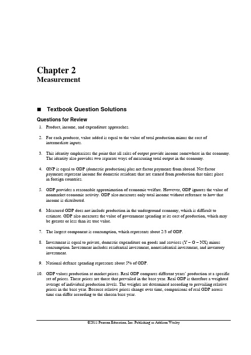
图1 1980-2007年转型国家人均GDP变动
资料来源:IMF 3
2007
第二章
2
$10,000 $9,000 $8,000 $7,000 $6,000 $5,000 $4,000 $3,000 $2,000 $1,000 $0
1980
1591 1494 1799 2052 2037 1895 1961 1687 1815 1768 1625 2310 2346 2101 2114 1866 1239 4050 4059 3599 2686 2647 2740 1838 1775 2111 2992 2383 4441 4339 4423 4976 5180 4105 7946 9214 8655 8183
6
6、平衡预算与自动稳定器 a. Y*=(C0+I+G-ct0)/[1-c(1-t)] b.T=t0+t1Y* c.假设政府实行平衡预算,且C0下降: 自主消费减少导致均衡产出减少,产出减少 引起税收减少。为了保持平衡预算,政府支 出也将减少。C0↓→Y↓→T↓→G↓→Y↓ d.政府支出减少加强了C0下降对产出的不利 影响。 因此,政府的平衡预算导致了经济的不稳定。
10
8.货币流通速度 货币交易方程:MV=PY M:货币存量 V:货币流通速度:每一元货币循环的次数。 P:物价水平 Y:实际收入 PY:名义收入
PY PY V M 0.8 4i
利率上升,货币 流通速度加快。
11
9、货币乘数(P85) 已知:cr=C/D=0;rr=R/D=0.1 a.已知高能货币供给为1000亿,货币供给量实际上 就是经济中存在的货币量,即货币供给必然等于货 币需求,因此高能货币需求也为1000亿。 b.高能货币(基础货币)的需求: Bd=C+R=0+R=R=rr×D 又货币需求:Md=C+D=D。代入上式得到基础货币需 求:Bd=rr×Md。 高能货币供给Bs=1000亿,收入为5万亿元,并将货 币需求函数一起代入Bs=Bd,得到:i=15% c.货币供给=1000/rr=10000 与货币需求相等。 d.Ms=3000/rr=Md可以计算出利率。 e.Ms=3000=Md可以计算出利率。
2. 重 新 考 虑 乘 数
d1和d 2分别是货币需求的收入弹性和利率弹性。
13
d .乘数
1 b2 d1 (1 c1 b1 ) d2
,
b2是投资的利率弹性,d 2是货币需求的利率弹性。 b2和d 2的变化使乘数不确定。 例如:假设b2不变,当d 2 0, 乘数 0; 1 1 当d 2 , 乘数 1 c1 b1 1 c1
8
货币需求和债券需求 a.债券需求=财富-货币需求 因此, 利率上升,货币需求减少,债券需求增 加。 b.财富=债券持有量+货币持有量 c.收入增加导致货币需求增加,债券需 求减少。
9
7.自动取款机和信用卡(P84) a.4×4=16 b.平均每天持有货币:(16+12+8+4)/4=10 自动取款机出现,每两天取一次钱: c.2×4=8 d.平均每天持有货币:(8+4)/2=6 信用卡出现,第四次取出所有的钱: e.每天持有货币量:0,0,0,16 f.平均每天持有货币: 16/4=4 g.自动取款机和信用卡的出现减少了人们 对通货的持有量。
14
4(P107)、货币与财政政策:一个例子 a.IS曲线:Y=C+I+G =200+0.25(Y-T)+150+0.25Y-1000i+250 =550+0.5Y-1000i得到:Y=1100-2000i b.LM曲线:M/P=L(Y,i)得到:Y=800+4000i c和d.联立IS与LM得到:i=0.05,Y=1000。 e.C=200+0.25(1000-200)=400,I=350。 f.LM:1840=2Y-8000i→ Y=920+4000i 联立IS得到:Y=1040,i=0.03,C=410,I=380 同理可以计算g和h。
第七章 AS-AD模型
1(176).对,对,错,错,对,错, 错。 2.支出冲击和中期
货币政策作用机制: M↑→(M/P)↑→i↓→I↑→Y↑→P↑→( M/P) ↓→LM返回
i
LM
a.消费者信心增加→消费增加→ IS、 AD右移→中期产出不变,价格和利率 上升。 b.税收增加导致消费减少,变化正好 相反。 4.货币中性 i a.货币变动在中期对实际变量(产出 和就业)没有影响,只是导致价格同 比例变化。货币政策在短期有影响。 b.财政扩张在中期对产出没有影响, 但是导致利率上升,挤出投资,贸易 赤字(财政扩张导致货币升值)。
4
第三章 物品市场
1(P61).对,对,错,对,错,错,错。 4.平衡预算乘数(P62) 平衡预算:△G=△T,即支出和收入等量变化。 Y=C+I+G= C0 +c(Y-T)+I+G得到: 均衡产出:Y=(C0+I+G-cT)/(1-c) a.△YG= △G /(1-c)= 1/(1-c) b. △YT=-c △T /(1-c)= -c/(1-c) c.税收增加导致可支配收入减少,消费减少。 d. △G=△T=1 则△Y= △YG + △YT=1 因此平衡 预算乘数等于1。没有保持宏观经济中性。 e. 无影响。因为平衡预算乘数为1,是个常数。
IS
Yn
Y
LM
IS
财政政策的作用机制: G↑→Y↑→P↑→(M/P)↓→i↑→I↓ →Y↓→回到自然产出。