LMI工具箱介绍——俞立
用线性矩阵不等式方法求解控制理论问题_张怡
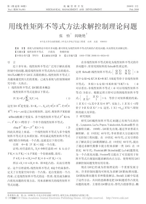
(a)包覆不完全
(b)形成间隙
图 1 粘结剂对炸药的润湿状况
(2)对于水悬浮法,造粒过程有水存在,此时发生 自动铺展的条件为:△G= γEB+ γBW- γEW< 0。 式中:γEB、γBW、γEW 分别为炸药- 粘结剂、粘结剂- 水、炸 药- 水界面张力。如果粘结剂满足在空气中能够完全 润湿炸药的条件,则上式可整理为:
- 1/2 - 1/2
其中,λmax (X,Y) 表示矩阵Y XY 的最大特征值。
GEVP是半凸(quasiconvex) 优化问题。
-1
(4)凸问题 (CP):minlodet A(X) , s.t A(X) > 0,
B(X) > 0。
(9)
这里A、B是仿射依赖于变量X的对称矩阵,注意当A>0
-1
等式问题。
在非线性矩阵不等式转化为线性矩阵不等式的许
多问题中,常常用到矩阵的Schur补性质定理。
# $ 定理(Schur补)线性矩阵不等式:
Q(X) S(T X)
S(X) R(X)
(3)
其中Q(X)=Q(X)T,R(X)=R(X)T,S(X)是等价于非线性矩阵
不等式: R(X) > 0,Q(X)- S(X)R(X)-1S(X)T> 0。 (4)
该步骤,直至收敛到问题的最优解。该算法虽简单,但
ห้องสมุดไป่ตู้
效率不高,仅适用于较小规模问题。
1988年,Nesterov和Nemirovskii提出了内点法,用
来求解具有线性矩阵不等式约束的凸优化问题,取得
了良好的效果。其基本思想是:运用约束集定义一个
凸的障碍函数,将其附加到原问题的目标函数中,以
一个无约束优化问题代替原有的约束优化问题,运用
Matlab LMI工具箱在教学和科研中的应用

第4 期
电气电子教学学报
J OUR NAL OF E E E
Vo . 4 No 4 13 . Au . 01 g2 2
21 02年 8月
MalbL t MI a 工具 箱 在 教 学 和 科研 中的应 用
江 兵 , 建 国, 郝 潘 平
( 合肥 工业 大学 电气 与 自动化 工程 学院 , 安徽 舍肥 200 ) 30 9
统 问题 。
1 系 统可行 性 问题 )
“
识、 电力系统和经济管理等诸多领域 的一个强大 的 设计 工具 。由于这 些领 域的许 多 问题 都 可 以转化 为
一
寻找一个 xR ( e 或等价为具有给定结构的矩 阵 瓦 )使 得满 足线性 矩 阵不等 式 系统 A( < , )
,
个 L 系统 的可行 性 问题 , 者是 一 个 具 有 L MI 或 MI
B( , )相应 的求 解 器 是 fap es。求 解 器 fap是 通过 es 求 解如 下的一 个辅 助 凸优 化 问题来求 解 线性矩 阵 不 等 式 系统 的 可行性 问题 的 。
mi L 来 解 决这 些 问题 已经 应 MI 成 为这些 领域 中的一 大 研究 热 点 。在 我校 “ 棒 控 鲁 制 ” “ 络 控 制 系 统 ” 课 程 教 学 和科 研 中 ,MI 和 网 等 L 工 具箱 正发挥 着越 来越 大 的作 用 0
St ( ..A )一B ) ( ≤I
1 L MI求解 器 简 介
L 工具 箱提供 的求 解器 用来求 解 以下 三类 系 MI
这个 凸优化 问题 的全局 最优值 用 tn a r表示 , 为 i 作 求 解器 fa es 出的第一 个分 量 。如果 t < , 系 p输 0则
LMI工具箱介绍俞立

function mainfunct 2;1 -3];
% 输入已知矩阵
A2=[-0.8 1.5;1.3 -2.7];
A3=[-1.4 0.9;0.7 -2];
setlmis([])
% 开始设置系统框架
11/26
机动 目录 上页 下页 返回 结束
P=lmivar(1, [2 1]) lmiterm([1 1 1 P], 1, A1, 's' ) lmiterm([2 1 1 P], 1, A2, 's' ) lmiterm([3 1 1 P], 1, A3, 's' ) lmiterm([-4 1 1 P],1,1) lmiterm([4 1 1 0],1) lmisys=getlmis [tmin,xfeas]=feasp(lmisys); PP=dec2mat(lmisys,xfeas,P)
③描述该项是变量还是常数. ④变量旳左系数、右系数. ⑤可选项, 只能是's' , 描述转置.
6/26
机动 目录 上页 下页 返回 结束
使用LMI工具箱描述
AT
X
XA BT X
C T SC
XB
S
0
X 0
SI
其中X∈R6×6 和 S = DTD∈R 4×4,
d1 D
d1
d2 d4
1、可行性问题 寻找一种x∈RN, 使得满足LMI
A(x) < B(x) 相应旳求解器是feasp. 一般体现形式
[tmin, xfeas]=feasp(lmisys, options, target) 原理:经过求解如下旳辅助优化问题
min t s.t. A(x)-B(x) ≤ tI 来求解线性矩阵不等式系统lmisys旳可行性问题.
LMI工具箱介绍
LMILMILMILMIL(x) L x L x L0(1)0 1 1 N NL0 , , , x1, , x NL L1 Nx[x1 , , ] R NxTN11L, , ) ( , , (X1 X n R X X n1 )L( ) R( ) X, ,1 Xn1LyapunovA T X XA0(2)XA1222 1x x1 22 X X 2x x2 3X x1 x x X2 3X1 0 0 1x1 x x2 30 0 1 01A 22 2 03 0 0x1 x x0(3)2 32 034 0 42 1 Lyapunov2 3 32 A n 3n(n1) 2LMI Lyapunov2 X 3HA X T XA X CTBNTCX I D N0BT DTIA X X T R n n RB C D NNA XT XA XCTBL(X, ) CX I DBT DTIX 1 1 L(X, ) L(X, )L(X, ) XL(X, ) B DXA, IA.2LMIN L(X, , X)N M R(X, , X)MT T1 K 1 KX1 , , N MXKL( ) R( )X0X00X1 2X, ,1XKlmisys lmisys LMIlmidem1 4 4 6G(s) C(s I A) 1 B(4)/ Dd10 0 00 d0 01D(5)0 0 d d2 30 0 d4 d 55 D sup DG( j)D 1 1 X R6 6 S D T D R4 4A T X XABTXC SCTXBS0(6)X0(7)S I(8)lmivar lmiterm 6 ~ 8 setlmis([])X=lmivar(1,[6 1])S=lmivar(1,[2 0;2 1])% 1st LMIlmiterm([1 1 1 X],1,A,’s’)lmiterm([1 1 1 S],C’,C)lmiterm([1 1 2 X],1,B)lmiterm([1 2 2 S],-1,1)% 2nd LMIlmiterm([-2 1 1 X],1,1)% 3rd LMIlmiterm([-3 1 1 S],1,1)lmiterm([3 1 1 0],1)lmisys=getlmislmivar X S lmitermgetlmis lmisys lmisyssetlmis getlmissetlmis getlmissetlmis([])lmisosetlmis(lmiso)lmisys=getlmislmisyslmivarlmivarX=lmivar(type,struct)XXtype XstructXType =1 D10 D 2DrDjstruct r 2i(m , n ) mDin 1 0 1 n 1Din 0Dn1DiiType =2 struct= (m , n )Type =3 X0 xnxnnstruct X0,X (i , j ) 0struct (i , j )n , X (i , j ) xnn ,X (i , j ) xn2 X 1 X2X3X3 3 1X 2 42X30 0 5 511 2I 20 0I2 22 2lmivarsetlmis([]) X1=lmivar(1,[3 1]) X2=lmivar(2,[2 4]) X3=lmivar(1,[5 1;1 0;2 0])lmiterm12 3 A T X C T SCPXQ X P Q3LMIlmitermA X T XAB XTC SCTXBSlmiterm([1 1 1 X],1,A,’s’)lmiterm([1 1 1 S],C’,C)lmiterm([1 1 2 X],1,B)lmiterm([1 2 2 S],-1,1)A T X XA C T SC XB S 11 m m-m m2 3 [1 1 2 1]1 2 2 30 k k X-k k 1X X T X 1 S 2k klmiterm 2 3 PXQ PX T Q4 's'12 lmiterm 's' lmitermA T X XA3 I1 3 S Ilmiterm([-3 1 1 S],1,1)lmiterm([3 1 1 0],1)lmivarnewlmi lmiterm1setlmis([])X=lmivar(1,[6 1])S=lmivar(1,[2 0;2 1])BRL=newlmilmiterm([BRL 1 1 X],1,A,’s’)lmiterm([BRL 1 1 S],C’,C)lmiterm([BRL 1 2 X],1,B)lmiterm([BRL 2 2 S],-1,1)Xpos=newlmilmiterm([-Xpos 1 1 X],1,1)Slmi=newlmilmiterm([-Slmi 1 1 S],1,1)lmiterm([Slmi 1 1 0],1)lmisys=getlmisX S X S BRL Xpos Slmi 1 2 3 -Xpos 2 -X Xlmieditlmieditlmiedit1S R Glmivar struct2 MATLABA X TB XT XA X BI[A’*X+X*A X*B;B’*X -1]<0X Xlmivar/lmiterm view commandsdescribe…lmivar/lmitermMATLABMATLAB saveloadlmivar/lmiterm readdescribe the matrix variables describe the LMIs …lmivar/lmiterm writecreateMATLAB mylmi MATLAB mylmi mylmilmiterm0 1 lmiedit lmiterm lmieditX(A*X+B)’*C+C’*(A*X+B)(A+B)’*X+X’*(A+B)lmiterm lmiterm 1newlmi lmivarA.1 lmiedit 1A.1 lmieditA.3LMI lmiinfo lminbr matnbrlmiinfolmiinfolmiinfolmiinfo(lmisys)lmisys getlmislminbr matnbrmatnbr(lmisys)A.4LMI xX, ,1 Xkx RNX, ,1XkA(x) B(x)feaspmin cTxxs.t. A(x) B(x)mincxminxs.t. C(x) D(x) (9)0 B(x) (10)A(x) B(x) (11) gevpfeaspfeasp[tmin,xfeas]=feasp(lmisys,options,target)feaspmin ts.t. A(x) B(x) t Ilmisystmin feasptmin<0 lmisys lmisys feaspxfeas dec2mat lmisysfeasp target tmin tmin<targettarget=0 feaspoptions 5options(1)options(2)100options(3) options(3)= R0Nx2 R2ii 1xfeas R R109xoptions(4)J J t1%10options(5) options(5)=1 options(5)=0options(i)3P I PA1 P PA012T1A2 P PA013T2A3 P PA14T31 20.8 1.5A 1A, A,23131.32.71.4 0.7 0.92.0feaspsetlmis([]) P=lmivar(1,[2 1]) lmiterm([1 1 1 P],1,A1,’s’) % LMI #1 lmiterm([2 1 1 P],1,A2,’s’) % LMI #2 lmiterm([3 1 1 P],1,A3,’s’) % LMI #3 lmiterm([-4 1 1 P],1,1) % LMI #4: P lmiterm([4 1 1 0],1) % LMI #4: Ilmis=getlmisfeasp[tmin,xfeas]=feasp(lmis)tmin 3.1363 lmis dec2matPP=dec2mat(lmis,xfeas,P)P270.8 126.4 126.4 155.1PFrobenius 10 tmin 1[tmin,xfeas]=feasp(lmis,[0,0,10,0,0],-1)tmin1.1745 P( ) maxP 9.6912mincxmincx[copt,xopt]=mincx(lmisys,c,options,xinit,target)lmisysc xdefcxcmincxc T x coptxoptdec2matxoptmincx lmisys c xinit xopt X, , X mat2dec1 kxinit xinittarget x c T x targetoptions 5options(1) copt 10 2options(2) 100options(3) feaspoptions(4) JJ c T x5options(5) options(5)=1 options(5)=0options(i)mincx4minTrace (X)Xs.t. A T X XA XBB T X Q0X1 2 1 1 1 1 0A 3 2 1 , B0 , Q 1 3 121 2 1 1 0 12 36SchurminTrace (X)XA X XA Q XBTs.t. 0B X ITTrace(X) Xmincxmincx1setlmis([])X=lmivar(1,[3 1]) % Xlmiterm([1 1 1 X],1,A,’s’)lmiterm([1 1 1 0],Q)lmiterm([1 2 2 0],-1)lmiterm([1 2 1 X],B’,1)LMIs=getlmis2 Trace(X) c T x x Xc X X Ic=mat2dec(LMIs,eye(3))defcx3 mincx xopt copt=c’*xoptoptions=[1e-5,0,0,0,0][copt,xopt]=mincx(LMIs,c,options)1e-5 coptmincxSolver for linear objective minimization under LMI constraintsIterations : Best objective value so far12 -8.5114763 -13.063640*** new lower bound: -34.0239784 -15.768450*** new lower bound: -25.0056045 -17.123012*** new lower bound: -21.3067816 -17.882558*** new lower bound: -19.8194717 -18.339853*** new lower bound: -19.1894178 -18.552558*** new lower bound: -18.9196689 -18.646811*** new lower bound: -18.80370810 -18.687324*** new lower bound: -18.75390311 -18.705715*** new lower bound: -18.73257412 -18.712175*** new lower bound: -18.72349113 -18.714880*** new lower bound: -18.71962414 -18.716094*** new lower bound: -18.71798615 -18.716509*** new lower bound: -18.71729716 -18.716695*** new lower bound: -18.716873Result: feasible solution of required accuracybest objective value: -18.716695guaranteed relative accuracy: 9.50e-006f-radius saturation: 0.000% of R = 1.00e+009c T xx 4 mincx xoptXopt=dec2mat(LMIs,xopt,X)6.3542 5.8895 2.20465.88956.2855 2.2201Xopt2.2046 2.2201 6.0771gevpgevp[lopt,xopt]=gevp(lmisys,nlfc,options,linit,xinit,target)gevploptxxopt dec2matlmisys 1 6 ~ 88nlfc( ,)linit=xxxinit=gevpx( ,)( ,)xtarget( , x ) target options5 options(1) lopt10 2options(2) 100options(3) feaspoptions(4)JJ5options(5) options(5)=1 options(5)=0options(i)gevpA (x )B (x )A (x )B (x )0 B (x )0 B (x )B (x )B (x ) 01B x , ( )1gevpYA (x )Y 0 0 0,YB 1(x ), B x( )A (x )B (x ), B (x ) 0gevp5 3x (t ) A (t ),i i x(1, 2, 3),A V (x ) x T Px, (i 1, 2, 3)3Lyapunov i d V (x ) 3d tmins.t.I P A PT 1PA 1 PA PT2PA2PA PT 3PA3Pgevpsetlmis([]); P=lmivar(1,[2 1]) lmiterm([1 1 1 0],1) % P>I: Ilmiterm([-1 1 1 P],1,1) % P>I: P lmiterm([2 1 1 P],1,A1,’s’) % LFC #1 (lhs) lmiterm([-2 1 1 P],1,1) % LFC #1 (rhs) lmiterm([3 1 1 P],1,A2,’s’) % LFC #2 (lhs) lmiterm([-3 1 1 P],1,1) % LFC #2 (rhs) lmiterm([4 1 1 P],1,A3,’s’) % LFC #3 (lhs) lmiterm([-4 1 1 P],1,1) % LFC #3 (rhs)lmis=getlmisgevp[alpha,popt]=gevp(lmis,3)alpha = -0.122 0.122P5.58 8.358.35 18.64x mat2dec dec2matX1 X X2 3X1 X2 X3 mat2decxdec=mat2dec(lmisys,X1,X2,X3)lmisys lmisysmincx gevpmat2dec xinit X1 X X2 3xdec dec2mat k2X2=dec2mat(lmisys,xdec,2)dec2mat 2lmivarmatnbr decnbr decinfoA.5LMIevallmi showlmi4 mincx xoptevlmi=evallmi(LMIs,xopt)[lhs,rhs]=showlmi(evlmi,1)xopt 1 eig(lhs-rhs)ans=-2.0387e-04-3.9333e-05-1.8917e-07-4.6680e+01lhs-rhs xopt 1A.6LMI dellmi delmvar setmvarDellmidellmi1 lmisys Xnewsys=dellmi(lmisys,2)2newsys1 2S I3 2newlmi 1 BRL Xpos Slmi Slminewsys=dellmi(lmisys,Xpos)2 S IdelmvardelmvarA T X XA BW W TB T I0X X R4 4 W R2 4Tsetlmis([])X=lmivar(1,[4 1]) % XW=lmivar(2,[2 4]) % Slmiterm([1 1 1 X],1,A,’s’)lmiterm([1 1 1 W],B,1,’s’)lmiterm([1 1 1 0],1)lmisys=getlmisWnewsys=delmvar(lmisys,W)newsys LyapunovA T X XA I0setmvarsetmvarsetmvar1 G 1 G 1D S D T D S IS2I Snewsys=setmvar(lmisys,S,2)2 S3 S 22I newsysA X T XAB XT2C CTXB2IX02I I newsys=dellmi(newsys,3)newsys =dellmi(newsys,Slmi)Slmi newlmi 3A.7lmivar 1 230 xn x n nX XX X n X p n xx, ,1 n pxn1, , x X lmivar n p[X,n,sX]=lmivar(type,struct)n sX Xx, , 1 xnlmivar6X X1X2X X1 X23 3 2 2X1 X1 X2setlmis([])[X1,n,sX1]=lmivar(2,[2 3]) [X2,n,sX2]=lmivar(2,[3 2])sX1 sX2 X1 X2>>sX1sX1=1 2 34 5 6>>sX2sX2=7 89 1011 12sX2(1, 1)=7 X(1, 1) 722 Type3 X X1 X2[X,n,sX]=lmivar(3,[sX1,zeros(2);zeros(3),sX2])X>>sXsX=1 2 3 0 04 5 6 0 00 0 0 7 80 0 0 9 100 0 0 11 127 3 3 X 3 3 Toeplizy 1 y2y3Y y2 y1y2y 3 y2y1Y 3 3 Y X Y n 1 n 2 n 3 n XXsetlmis([])[X,n]=lmivar(1,[3 1])[X, n] 2 n=6 YY=lmivar(3,n+[1 2 3;2 1 2;3 2 1])Y=lmivar(3,toeplitz(n+[1 2 3]))toeplitz MATLAB decinfo X Ylmis=getlmisdecinfo(lmis,X)ans=1 2 42 3 54 5 6decinfo(lmis,Y)ans=7 8 98 7 89 8 78X Y ZX xy, Yzt, Ztxx y z tX Y 1setlmis([])[X,n,sX]=lmivar(1,[1 0;1 0])[Y,n,sY]=lmivar(1,[1 0;1 0])lmivar 3 X Y(x, , , )1x x x2 3 4 (x, y, z, t)sX=1 00 2sY=3 00 4lmivar 3 Z[Z,n,sZ]=lmivar(3,[0 -sX(1,1);-sY(2,2) 0])sX(1, 1) x sY(2, 2)1x4Zx4x1txHermitian matrix L(x) L(x) 0Re(L(x))Im(L(x))I m(L(x))Re(L(x))XX X1 j X2X1 X2AA A j1 A2A 1 A 2X1 X2X1 X2 X2X1XX1 j X2 A1A2A2A1A A1 j A2M H XM X, X X H IM1M2T X1X2M1M2X1X2 M2M1X2X1M2M1X2X1X1X2X2X1IM 1 j MM2X X1 j X2Mi XiM C55M1=real(M), M2=imag(M)bigM=[M1 M2;-M2 M1]setlmis([])% declare bigX=[X1 X2;-X2 X1] with X1=X1’ and X2+X2’=0:[X1,n1,sX1]=lmivar(1,[5 1])[X2,n2,sX2]=lmivar(3,skewdec(5,n1))bigX=lmivar(3,[sX1 sX2;-sX2 sX1])% describe the real counterpart of the complex LMI system:lmiterm([1 1 1 0],1)lmiterm([-1 1 1 bigX],1,1)lmiterm([2 1 1 bigX],bigM’,bigM)lmiterm([-2 1 1 bigX],1,1)lmis=getlmisbigX= X1X2X2X11 X sX11n1 X12 skewdec X skewdec(5,n1)2n1+1, n1+2, ... 5 53 3 X X sX1, sX2 bigX1 2mincx c T xmincx c T x xTrace(X) X u T Xu udefcx cTrace(X) x PxT0 0X P x lmisysX Pxx0=[1 1]setlmis([])X=lmivar(1,[3 0])P=lmivar(1,[2 1])::lmisys=getlmisc T x Trace(X) x Px cT0 0n=decnbr(lmisys)c=zeros(n,1)for j=1:n,[Xj,Pj]=defcx(lmisys,j,X,P)c(j)=trace(Xj)+x0’*Pj*x0end1 2 cfor1 x 1 x X P defcx defcxjlmisys j X PXj Pj2 X=Xj P=Pj c jc=3121n=decnbr(LMI system)c=zeros(n,1)for j=1:n,[matrix values]=defcx(LMI system,j,matrix identifiers)c(j)=objective(matrix values)endA.8 系统模型描述Ex(t) y(t) Ax(t)Cx(t)Bu(t)Du(t)(15)A, B, C, D, E E x(t), u(t), y(t)15E15 E15mx fx kx uy x151 0 0m(t)k1f(t)1u(t) y(t) 1 0 (t)(t) [x(t) x(t)]T15 MATLAB SYSTEMn A j(E I) B0C D00 InfnLMI ltisys ltiss SYSTEM SYSTEMsys=ltisys(-1,1,1,0)x x u, y xSYSTEM SYSTEM sys A, B, C, D [A,B,C,D]=ltiss(sys)ltitf SYSTEM G(s) n(s)d(s)sys=ltisys(‘tf’,n,d)G(s) n d n(s) d(s)sinfo(sys) SYSTEM sysspol(sys) ssubSYSTEM G G 12 3ssub(G,1,2:3)G G SYSTEM sinv G(s) H(s) G 1 (s)G(s) D sbalancA, B, CLMISYSTEMSYSTEMg1 g2 G1(s) G2 (s) SYSTEM saddG1 s( )( ) G2 s SYSTEM smult(g1,g2)SYSTEM 10 G( ) ( ) 2s G s1sdiag(g1,g2) G(s) diag{G1(s), G2 (s)} SYSTEMSr+yG1(s)G2(s)1sloop r y SYSTEMslft w1w2z1z2SYSTEMw1u G1(s) z1 yz2G2(s) w22u R2 , y R3slft(g1,g2,2,3)H。
MATLABLMI工具箱使用教程算例及论文原文.pdf
Abstract
In this paper, we consider the problem of designing H state feedback controller for the generalized time-delay systems with delayed states and control inputs in continuous and discrete time cases, respectively. The generalized time-delay system problems are solved on the basis of linear matrix inequality (LMI) technique considering time delays. The su$cient condition for the existence of controller and H state feedback controller design methods are presented. Also, using some changes of variables and Schur complements, the obtained su$cient condition can be rewritten as an LMI form in terms of transformed variables. The proposed controller design method can be extended into the problem of robust H state feedback controller design method easily. 1999 Elsevier Science Ltd. All rights reserved.
Matlab中的LMI工具箱的研究与使用

Matlab中的LMI工具箱的研究与使用Matlab中的LMI工具箱的研究与使用摘要:由于内点算法可以利用计算机求解高阶矩阵不等式,使得线性矩阵不等式(LMI)在控制理论得以应用,因而线性矩阵不等式在控制系统分析、设计中扮演着越来越重的角色。
在毕业设计中,我学习了LMI理论,Matlab中LMI工具箱的使用,研究了常见的控制问题与LMI关系以及其表达式,并研究了基于LMI方法的鲁棒控制器设计问题,推导了如何将鲁棒控制器设计问题转化为LMI形式,给出了通过求解LMI方程构造控制率的算法。
LMI是一种较新的方法,可以在控制系统的许多领域得以应用,如鲁棒控制、非线性控制预测控制等有着巨大的潜力。
关键词:线性矩阵不等式;LMI工具箱;控制系统The research and use of the Matlba LMI toolboxStudent majoring in Automation SUN Peng-kunTutorAbstract:Due to the interior point algorithm can use computer to solve high order matrix inequality,It makes the linear matrix inequality (LMI) in the control theory to application and linear matrix inequality (LMI) played more and more heavy role in the control system analysis and design. At the graduation design, I studied the LMI theory, in the use of Matlab LMI toolbox, and studies the problem of common control with LMI relations and its expression,and I studied the problem of the robust contoeller design that based on lmi method, how totransform the robust controller design problem into the LMI form, and given by solving the LMI equation of tectonic control algorithm. LMI is a new method, it can be used in many control system fields, such as robust control, nonlinear control predictive control, and it has great potential.Key words: linear matrix inequality; LMI toolbox; control system;robust control引言线性矩阵不等式(LMI)工具箱是求解一般线性矩阵不等式问题的一个高性能软件包。
matlab lmi工具箱使用实例
MATLAB(Matrix Laboratory)是一款广泛应用于科学计算和工程领域的专业软件,其功能强大、灵活性高,并且具有丰富的工具箱支持。
LMI(Linear Matrix Inequality)工具箱是MATLAB中的一种工具箱,用于解决线性矩阵不等式相关的问题。
本文将介绍LMI工具箱的基本使用方法,并结合具体实例进行详细讲解。
一、LMI工具箱的安装1.确保已经安装了MATLAB软件,并且软件版本是R2015b及以上版本。
只有在这些版本中,LMI工具箱才会被自动安装。
2.在MATLAB的命令行中输入“ver”,可以查看当前安装的工具箱列表,确认LMI工具箱是否已经成功安装。
二、LMI工具箱的基本功能1. LMI工具箱主要用于解决线性矩阵不等式问题,例如矩阵的稳定性分析、最优控制问题等。
2. LMI工具箱提供了一系列的函数和工具,能够方便地构建和求解线性矩阵不等式问题,同时也包括了一些经典的稳定性分析方法和控制器设计方法。
三、LMI工具箱的基本使用方法1. 定义变量:在使用LMI工具箱时,首先需要定义相关的变量。
可以使用“sdpvar”函数来定义实数变量,使用“sdpvar”函数和“size”函数可以定义矩阵变量。
2. 构建约束:在定义变量之后,需要构建线性矩阵不等式的约束条件。
可以使用“sdpvar”变量的线性组合来构建约束条件,使用“>=”来表示大于等于关系。
3. 求解问题:构建好约束条件之后,即可使用“optimize”函数来求解线性矩阵不等式问题。
在求解问题时,可以指定优化的目标函数和一些额外的约束条件。
四、LMI工具箱的实例应用下面我们通过一个具体的实例来演示LMI工具箱的使用方法。
假设有一个线性时不变系统,其状态方程可以表示为:$\dot{x} = Ax + Bu$其中,A和B分别为系统的状态矩阵和输入矩阵。
我们希望设计一个状态反馈控制器K,使得系统在闭环下能够保持稳定。
LMI工具箱介绍——俞立
LMI⼯具箱介绍——俞⽴LMI ⼯具箱介绍线性矩阵不等式(LMI )⼯具箱是求解⼀般线性矩阵不等式问题的⼀个⾼性能软件包。
由于其⾯向结构的线性矩阵不等式表⽰⽅式,使得各种线性矩阵不等式能够以⾃然块矩阵的形式加以描述。
⼀个线性矩阵不等式问题⼀旦确定,就可以通过调⽤适当的线性矩阵不等式求解器来对这个问题进⾏数值求解。
LMI ⼯具箱提供了确定、处理和数值求解线性矩阵不等式的⼀些⼯具,它们主要⽤于:z 以⾃然块矩阵形式来直接描述线性矩阵不等式; z 获取关于现有的线性矩阵不等式系统的信息; z 修改现有的线性矩阵不等式系统; z 求解三个⼀般的线性矩阵不等式问题; z 验证结果。
本附录将详细介绍LMI ⼯具箱提供的⽤于解决以上各个问题的相关函数和命令。
A.1 线性矩阵不等式及相关术语⼀个线性矩阵不等式就是具有以下⼀般形式的⼀个矩阵不等式:0<+++=N N x x L L L x L "110)( (1)其中:是给定的对称常数矩阵,是未知变量,称为决策变量,N L L L ,,,10"N x x ,,1"∈=T 1],,[N x x "x N R 是由决策变量构成的向量,称为决策向量。
尽管表达式(1)是线性矩阵不等式的⼀个⼀般表⽰式,但在⼤多数实际应⽤中,线性矩阵不等式常常不是以⼀般表⽰式(1)的形式出现,⽽是具有以下形式:),,(),,(11n n X X R X X L ""<其中的和是矩阵变量的仿射函数,通过适当的代数运算,上式可以写成线性矩阵不等式的⼀般表⽰式(1)的形式。
例如,在系统稳定性问题中经常遇到的Lyapunov 矩阵不等式)(?L )(?R n X X ,,1"0<+XA X A T (2)也是⼀个线性矩阵不等式,其中的是⼀个矩阵变量。
我们以⼀个⼆阶矩阵为例,将矩阵不等式(2)写成⼀般表⽰式(1)的形式。
基于“自动控制原理”与“现代控制理论”课程异同点分析的教学探索
摘要本文分析了两课程异同点,并给出了应对方法。
提出合理选取教材和分配学时、弱化理论证明等降低理论难度;介绍人物故事、开展双语教学、强化实验等提高学习兴趣;采用比较教学新方法应对教学内容差异。
文末指出探索的新方向。
关键词现代控制理论自动控制原理教学实践比较教学法Exploration on Teaching Based on Analysis of Similarities and Differences between"Automatic Control Theory"and "Modern Control Theory"Courses//Wan Xiongbo,YangFangAbstract This paper analyzes the similarities and differences be-tween the above two courses and gives the corresponding meth-ods.To reduce theoretical difficulties,the methods such as se-lecting appropriate textbooks,suitable distribution of teachinghours,and simplifying the complexity of theory proof,are expect-ed;To improve students'interest in learning,the methods includ-ing introduction of scientists biographies,bilingual education,and strengthening the experiments,are proposed;Compari-son-based new teaching method is utilized to deal with the dif-ferences between the contents of two courses.Finally,new direc-tions for future exploration are discussed.Key words modern control theory;automatic control theory;teaching practice;comparison-based teaching method “自动控制原理”是研究控制系统的一般规律,并为系统的分析和综合提供基本理论和方法的专业基础核心课程[1,2]。
LMI工具箱介绍
L M IL M IL M IL M I0NN x x L L L x L 110)( (1)NL L L ,,,10Nx x ,,1T1],,[N x x x N R11),,(),,(11n n X X R X X L1Lyapunov)(L )(R nX X ,,10XA X A T (2)21X221A22X3221x x x x X X321x x x X100001100001321x x x XA20400043300222321x x x (3) 21Lyapunov23323A n2)1(n n L M ILyapunov23XH0NID B D ICX BXC XA X A N TTTT TNDCBAT XXnnR RNI D B D I CX B XC XA X A X L TT TT ),(X 11),(X L ),(X L),(X L X),(X L BDIXA ,A.2L M IM X X R M NX X L N ),,(),,(1T 1T K KKX X ,,1N M)(L )(R 0XXX1KX X ,,12l m i s y s l m i s y sL M Il m i de m1446B A IC G 1)()(s s (4)/D543211000000000d d d d d d D(5)5D1)(s up 1DDG jX66R DD ST 44R0S XB XB SC C XA XA T T T (6) 0X (7) I S(8)l m i var l m it er m 6~8setlmis([])X=lmivar(1,[6 1]) S=lmivar(1,[2 0;2 1])% 1st LMIlmiterm([1 1 1 X],1,A,’s’) lmiterm([1 1 1 S],C’,C) lmiterm([1 1 2 X],1,B) lmiterm([1 2 2 S],-1,1) % 2nd LMI lmiterm([-2 1 1 X],1,1)% 3rd LMI lmiterm([-3 1 1 S],1,1) lmiterm([3 1 1 0],1) lmisys=getlmisl m i varX l m it er mge tl m i sl m i s ys l m i s y sSs et l m i sget l m i s s e tl m i s ge tl m i ssetlmis([])l m i s osetlmis(lmiso) lmisys=getlmisl m i s y sl m i varl m i varX=lmivar(type,struct)X Xt ype Xs t ruc tX Type =1rD D D 0000021s t ruc tjD 2r in 10),(n m miD 11n i D 0n iD 1niD Type =2s t ruc t = ),(n m Type =3X0nx s t ruc tnx nXs t ruc tnn x j i n x j i n j i j i ),(,),(,0),(,0),(X X X 221X X3X1X 332X 42 2213I X 0000055122I 22l m i varsetlmis([])X1=lmivar(1,[3 1]) X2=lmivar(2,[2 4]) X3=lmivar(1,[5 1;1 0;2 0])l m i term1 23X A T S CC T P X QXPQ 3L M Il m it er m0SXB XB S CC XA X A TT Tlmiterm([1 1 1 X],1,A,’s’) lmiterm([1 1 1 S],C’,C) lmiterm([1 1 2 X],1,B) lmiterm([1 2 2 S],-1,1)XB S CC XA XA T T S11mm -m m23[1 1 2 1]1223k k-k 1kX k X T k X X 12S l m it er m234's 'P X Q QP X T1 2l m it er m's 'l m it er mXA X A T3I13I S lmiterm([-3 1 1 S],1,1) lmiterm([3 1 1 0],1)l m i varnew l m il m it er m1setlmis([]) X=lmivar(1,[6 1]) S=lmivar(1,[2 0;2 1])BRL=newlmilmiterm([BRL 1 1 X],1,A,’s’) lmiterm([BRL 1 1 S],C’,C) lmiterm([BRL 1 2 X],1,B) lmiterm([BRL 2 2 S],-1,1) Xpos=newlmi lmiterm([-Xpos 1 1 X],1,1)Slmi=newlmi lmiterm([-Slmi 1 1 S],1,1) lmiterm([Slmi 1 1 0],1) lmisys=getlmisX SX BR L Xpo s Sl m i123-Xpo s2-XSXl m i e di tl m i ed itlmiedit1SRGl m i vars t ruc t2M ATLA B0IXB XBXA X A T T[A’*X+X*A X*B;B’*X -1]<0X Xl m i var /l m it er m v i ew co mm and sde s cr i be…l m i var /l m it er mM ATLA BM ATLA B s avel oadl m i var /l m it er m readde s cr i be t he m a t r i x var i ab l e s de s cr i be t he L M I s …l m i var /l m it er m wr it e crea t eM ATLA B m y l m i M ATLA B m y l m i m y l m il m it er m01l m i ed itl m it er m l m i ed it X (A*X+B)’*C+C’*(A*X+B)(A+B)’*X+X’*(A+B)l m it er m l m it er m1new l m i l m i varA.1l m i ed it1A.1l m i ed itA.3L M I l m ii nfo l m i nbr m a t nbrl m iin fol m ii nfol m ii nfolmiinfo(lmisys)l m i s y s ge tl m i sl m inb r mat nb rmatnbr(lmisys)A.4L M I xkX X ,,1NR x kX X ,,1)()(x B x Afea s px c xT m i ns .t . )()(x B x Am i ncxxm i ns .t . )()(x D x C (9))(x B 0(10) )()(x B x A (11)gevpfea s pfea s p[tmin,xfeas]=feasp(lmisys,options,target)fea s pt m i ns .t . I x B x A t )()( l m i s y st m i nfea s pt m i n <0l m i s y sl m i s y s fea s pxfea sdec2m a tl m i s y s fea s pt arge t t m i n t m i n <t arge tt arge t =0fea s pop ti on s5op ti on s (1)op ti on s (2)100 op ti on s (3)op ti on s (3)=R212R x N i ixfea sR910Rxop ti on s (4)J1%10Jt op ti on s (5)op ti on s (5)=1op ti on s (5)=0op ti on s (i )3IPP01T 1P A PA 1202T 2P A PA 13 03T 3P A P A 14.27.09.04.1,7.23.15.18.0,3121321A A A fea s psetlmis([]) P=lmivar(1,[2 1])lmiterm([1 1 1 P],1,A1,’s’) % LMI #1 lmiterm([2 1 1 P],1,A2,’s’) % LMI #2 lmiterm([3 1 1 P],1,A3,’s’) % LMI #3 lmiterm([-4 1 1 P],1,1) % LMI #4: P lmiterm([4 1 1 0],1)% LMI #4: Ilmis=getlmisfea s p[tmin,xfeas]=feasp(lmis)t m i n l m i sdec2m a t1363.3PP=dec2mat(lmis,xfeas,P)1.1554.1264.1268.270PPF roben i u s10t m i n1[tmin,xfeas]=feasp(lmis,[0,0,10,0,0],-1)t m i n1745.1P6912.9)(m axPm in cxm i ncx[copt,xopt]=mincx(lmisys,c,options,xinit,target)l m i s y s cxdefcxcm i ncxcop txop tdec2m a txop tx c Tm i ncx l m i s y sc x i n it xop tm a t 2decx i n itx i n itkX X ,,1t arge t t arge txxc T op ti on s 5op ti on s (1)cop t210op ti on s (2)100op ti on s (3)fea s pop ti on s (4)5JJx c T op ti on s (5)op ti on s (5)=1op ti on s (5)=0op ti on s (i)m i ncx4)(Trace m i n X Xs .t .0Q X XBB XA XA T T X36121231011,101,121123121Q B AS chur)(Trace m i n X Xs .t .0IXB XB Q XA XA TT )(Trace X Xm i ncxm i ncx1setlmis([])X=lmivar(1,[3 1]) % Xlmiterm([1 1 1 X],1,A,’s’)lmiterm([1 1 1 0],Q)lmiterm([1 2 2 0],-1)lmiterm([1 2 1 X],B’,1)LMIs=getlmisTrace X x c T x X2)(c X I Xc=mat2dec(LMIs,eye(3))defcx3m i ncx xop t cop t=c’*xop toptions=[1e-5,0,0,0,0][copt,xopt]=mincx(LMIs,c,options)1e-5cop tm i ncxSolver for linear objective minimization under LMI constraints Iterations : Best objective value so far12 -8.5114763 -13.063640*** new lower bound: -34.0239784 -15.768450*** new lower bound: -25.0056045 -17.123012*** new lower bound: -21.3067816 -17.882558*** new lower bound: -19.8194717 -18.339853*** new lower bound: -19.189417 8 -18.552558 *** new lower bound: -18.919668 9 -18.646811 *** new lower bound: -18.803708 10 -18.687324 *** new lower bound: -18.753903 11 -18.705715 *** new lower bound: -18.732574 12 -18.712175 *** new lower bound: -18.723491 13 -18.714880 *** new lower bound: -18.719624 14 -18.716094 *** new lower bound: -18.717986 15 -18.716509 *** new lower bound: -18.717297 16 -18.716695 *** new lower bound: -18.716873Result: feasible solution of required accuracy best objective value: -18.716695 guaranteed relative accuracy: 9.50e-006 f-radius saturation: 0.000% of R = 1.00e+009x c T x4m i ncxxop tXopt=dec2mat(LMIs,xopt,X)0771.62201.22046.22201.22855.65.88952046.28895.56.3542op tX gev pgevp[lopt,xopt]=gevp(lmisys,nlfc,options,linit,xinit,target)gevpl op tx xop t dec2m a tl m i s y s 16~88n l fcli n it =),(00x 0x i n it =gevpt arge tx ),(00x ),(00x ),(x t arge top ti on s5op ti on s (1)l op t210op ti on s (2)100op ti on s (3)fea s pop ti on s (4)JJ5op ti on s (5)op ti on s (5)=1op ti on s (5)=0op ti on s (i )gevp)()(x B x A)()(x B x A)(x B 0)(x B 00000)(,)()(11x B x B x BgevpY0000)(),(,)(1x B x B Y Y x A0)(),()(x B x B x Agevp53),3,2,1(),()(itt i x Ax3Lyapunov3)3,2,1(,i i A Px xx T)(VtVd)(d xm i ns.t. P IPP AP A1T1PP AP A2T2PP AP A3T3gevpsetlmis([]);P=lmivar(1,[2 1])lmiterm([1 1 1 0],1) % P>I: Ilmiterm([-1 1 1 P],1,1) % P>I: Plmiterm([2 1 1 P],1,A1,’s’) % LFC #1 (lhs)lmiterm([-2 1 1 P],1,1) % LFC #1 (rhs)lmiterm([3 1 1 P],1,A2,’s’) % LFC #2 (lhs)lmiterm([-3 1 1 P],1,1) % LFC #2 (rhs)lmiterm([4 1 1 P],1,A3,’s’) % LFC #3 (lhs)lmiterm([-4 1 1 P],1,1) % LFC #3 (rhs)lmis=getlmisgevp[alpha,popt]=gevp(lmis,3)a l pha =-0.1220.12264.1835.835.858.5Px m a t 2dec dec2m a tX1X2X3m a t 2dec321X X X xdec=mat2dec(lmisys,X1,X2,X3)l m i s y sl m i s y sm i ncx gevpm a t 2decx i n it321X X X xdecdec2m a tk2X2=dec2mat(lmisys,xdec,2)dec2m a t2l m i varm a t nbrdecnbr dec i nfoA.5L M I eva ll m is how l m i4m i ncxxop tevlmi=evallmi(LMIs,xopt) [lhs,rhs]=showlmi(evlmi,1)xop t1eig(lhs-rhs)ans=-2.0387e-04-3.9333e-05-1.8917e-07-4.6680e+01l h s-rh s xop t1A.6L M I de ll m i de l m var s e t m varDe ll m ide ll m i1l m i s y s Xnewsys=dellmi(lmisys,2)2new s y s12I S32new l m i1BR L Xpo s Sl m i Sl m inewsys=dellmi(lmisys,Xpos)2I Sd e l mvarde l m var0I B W B W XA X A T T TT X X44R42R Wsetlmis([]) X=lmivar(1,[4 1]) % X W=lmivar(2,[2 4]) % Slmiterm([1 1 1 X],1,A,’s’) lmiterm([1 1 1 W],B,1,’s’) lmiterm([1 1 1 0],1) lmisys=getlmisWnewsys=delmvar(lmisys,W)new s y sLyapunov0I XA X A Ts e t m vars etmvars e t m var11G1G D DD ST IS I S2Snewsys=setmvar(lmisys,S,2)2S32S I 2new s y s0IXB XB CC XA XA 22TT T0X I I 2newsys=dellmi(newsys,3) newsys =dellmi(newsys,Slmi) Sl m i new l m i 3 A.7l m i var 123 0n x n x n X X X X n X p p n n x x ,,1p n n x x ,,1X l m i var[X,n,sX]=lmivar(type,struct) n s X X nx x ,,1l m i var 621X X X00 X1X 2X 3223X 1 1X 2Xsetlmis([])[X1,n,sX1]=lmivar(2,[2 3]) [X2,n,sX2]=lmivar(2,[3 2])s X1s X2 1X 2X>>sX1sX1=1 2 3 4 5 6>>sX2sX2= 7 89 10 11 12 s X2(1, 1)=7(1, 1)7 2X 2Type 3X 1X 2X [X,n,sX]=lmivar(3,[sX1,zeros(2);zeros(3),sX2]) X>>sXsX= 1 2 3 0 0 4 5 6 0 0 0 0 0 7 8 0 0 0 9 10 0 0 0 11 12 733X 33Toep li z123212321y y y y y y y y y Y Y 33Y X Y 321n n n n XXsetlmis([]) [X,n]=lmivar(1,[3 1]) [X, n]2n =6Y Y=lmivar(3,n+[1 2 3;2 1 2;3 2 1])Y=lmivar(3,toeplitz(n+[1 2 3])) t oep lit zM ATLA B dec i nfo X Ylmis=getlmis decinfo(lmis,X) ans= 1 2 4 2 3 5 4 5 6decinfo(lmis,Y)ans= 7 8 9 8 7 8 9 8 78Y X Z00,00,00t x t z y x Z Y X tz y x X Y1 setlmis([])[X,n,sX]=lmivar(1,[1 0;1 0]) [Y,n,sY]=lmivar(1,[1 0;1 0])l m i var 3X Y),,,(4321x x x x ),,,(t z y x sX=1 0 0 2sY=3 0 04 l m i var 3Z[Z,n,sZ]=lmivar(3,[0 -sX(1,1);-sY(2,2) 0]) s X(1, 1)s Y(2, 2) 1x 4x 000041t x x x ZHer m iti an m a t r i x)(x L 0)(x L 0))(R e())(I m ())(I m ())(R e(x L x L x L x L X21X X X j 1X 2X A21A A A j 1A 2A 21X X 1221X X X X X21X X j 1221A A A A 21A A A j I X X X X M M H H , 122112211221T 1221X X X X M M M M X X X X M M M M I X X X X 1221 21M M M j 21X X X j i i X M 55C M M1=real(M), M2=imag(M) bigM=[M1 M2;-M2 M1] setlmis([])% declare bigX=[X1 X2;-X2 X1] with X1=X1’ and X2+X2’=0:[X1,n1,sX1]=lmivar(1,[5 1])[X2,n2,sX2]=lmivar(3,skewdec(5,n1)) bigX=lmivar(3,[sX1 sX2;-sX2 sX1])% describe the real counterpart of the complex LMI system: lmiterm([1 1 1 0],1) lmiterm([-1 1 1 bigX],1,1)lmiterm([2 1 1 bigX],bigM’,bigM)lmiterm([-2 1 1 bigX],1,1)lmis=getlmis b i gX =1221X X X X 1s X1n1 1X 1X 2s kewdec s kewdec(5,n1)n1+1, n1+2, ... 2X 5533s X1, s X2b i gX 1X 2Xm in cxx c Tm i ncxx c T x )(Trace X XX uu T u defcx c0T 0)(Trace Px x X X P l m i s y s 0x P X x 0 x0=[1 1] setlmis([])X=lmivar(1,[3 0]) P=lmivar(1,[2 1]) : :lmisys=getlmis 0T 0T )(Trace Px x X x c c n=decnbr(lmisys) c=zeros(n,1) for j=1:n,[Xj,Pj]=defcx(lmisys,j,X,P) c(j)=trace(Xj)+x0’*Pj*x0end 12for c 11j x x X P defcx defcx l m i s y s j X P X j Pj 2X =X j P =Pj j cc=3 1 2 1n=decnbr(LMI system) c=zeros(n,1) for j=1:n, [matrix values]=defcx(LMI system,j, matrix identifiers) c(j)=objective(matrix values) end A.8 系统模型描述)()()()()()(t t t t t t D u C x y B u A x x E (15) E D C B A ,,,,E 15)(),(),(t t t y u x E 15E 15 x y u kx x f x m 15 )(01)()(10)(10)(001t t y t u t f k t mT ])()([)(t x t x t 15M ATLA B S Y S TE MInf 00)(0n j D CB I E An L M I lti s y s lti ss S Y S TE M S Y S TE Msys=ltisys(-1,1,1,0)x y u x x , SYSTEM SYSTEM sys DC B A ,,, [A,B,C,D]=ltiss(sys) ltitf SYSTEM )()()(s d s n s G sys=ltisys(‘tf’,n,d) n d )(s G )(s n )(s d sinfo(sys)SYSTEM sys spol(sys)ssub SYSTEM G 123 G ssub(G,1,2:3) G G SYSTEM sinv )(s G )()(1s s G H )(s G D sbalancC B A ,,L M I SYSTEM SYSTEMg1g2SYSTEM sadd )(1s G )(2s G)(1s G )(2s G SYSTEM smult(g1,g2)SYSTEM 10 )()(12s s G G sdiag(g1,g2)SYSTEMS )}(),({d i ag )(21s s s G G G G 1(s )G 2(s )y r + 1 sloop r y SYSTEM slft SYSTEM 21w w 21z z G 1(s )G 2(s )w 1u z 1y w 2z 2 232,R R y u slft(g1,g2,2,3) H。
- 1、下载文档前请自行甄别文档内容的完整性,平台不提供额外的编辑、内容补充、找答案等附加服务。
- 2、"仅部分预览"的文档,不可在线预览部分如存在完整性等问题,可反馈申请退款(可完整预览的文档不适用该条件!)。
- 3、如文档侵犯您的权益,请联系客服反馈,我们会尽快为您处理(人工客服工作时间:9:00-18:30)。
LMI 工具箱介绍线性矩阵不等式(LMI )工具箱是求解一般线性矩阵不等式问题的一个高性能软件包。
由于其面向结构的线性矩阵不等式表示方式,使得各种线性矩阵不等式能够以自然块矩阵的形式加以描述。
一个线性矩阵不等式问题一旦确定,就可以通过调用适当的线性矩阵不等式求解器来对这个问题进行数值求解。
LMI 工具箱提供了确定、处理和数值求解线性矩阵不等式的一些工具,它们主要用于:z 以自然块矩阵形式来直接描述线性矩阵不等式; z 获取关于现有的线性矩阵不等式系统的信息; z 修改现有的线性矩阵不等式系统; z 求解三个一般的线性矩阵不等式问题; z 验证结果。
本附录将详细介绍LMI 工具箱提供的用于解决以上各个问题的相关函数和命令。
A.1 线性矩阵不等式及相关术语一个线性矩阵不等式就是具有以下一般形式的一个矩阵不等式:0<+++=N N x x L L L x L "110)( (1)其中:是给定的对称常数矩阵,是未知变量,称为决策变量,N L L L ,,,10"N x x ,,1"∈=T 1],,[N x x "x N R 是由决策变量构成的向量,称为决策向量。
尽管表达式(1)是线性矩阵不等式的一个一般表示式,但在大多数实际应用中,线性矩阵不等式常常不是以一般表示式(1)的形式出现,而是具有以下形式:),,(),,(11n n X X R X X L ""<其中的和是矩阵变量的仿射函数,通过适当的代数运算,上式可以写成线性矩阵不等式的一般表示式(1)的形式。
例如,在系统稳定性问题中经常遇到的Lyapunov 矩阵不等式)(⋅L )(⋅R n X X ,,1"0<+XA X A T (2)也是一个线性矩阵不等式,其中的是一个矩阵变量。
我们以一个二阶矩阵为例,将矩阵不等式(2)写成一般表示式(1)的形式。
针对二阶矩阵不X ⎥⎦⎤⎢⎣⎡−−=2021A等式(2),对应的矩阵变量是一个二阶的对称矩阵,,不等式(2)中的决策变量是矩阵中的独立元。
根据对策性,矩阵变量可以写成X ⎥⎦⎤⎢⎣⎡=3221x x x x X X 321x x x 、、X ⎥⎦⎤⎢⎣⎡+⎥⎦⎤⎢⎣⎡+⎥⎦⎤⎢⎣⎡=100001100001321x x x X 将矩阵A 和上式代入矩阵不等式(2),经整理,可得0<⎥⎦⎤⎢⎣⎡−+⎥⎦⎤⎢⎣⎡−−+⎥⎦⎤⎢⎣⎡−400043300222321x x x (3) 这样就将矩阵不等式(2)写成了线性矩阵不等式的表示式(1)。
显然,与Lyapunov 矩阵不等式(2)相比,表示式(3)缺少了许多控制中的直观意义。
另外,(3)式涉及到的矩阵也比(2)式中的多。
如果矩阵是阶的,则(3)式中的系数矩阵一般有A n 2)1(+n n 个。
因此,这样的表达式在计算机中将占用更多的存储空间。
由于这样的一些原因,LMI 工具箱中的函数采用线性矩阵不等式的结构表示。
例如,Lyapunov 矩阵不等式(2)就以矩阵变量的不等式来表示,而不是用其一般形式(3)来表示。
X 一般的,一个线性矩阵不等式具有块矩阵的形式,其中每一个块都是矩阵变量的仿射函数。
以下通过一个例子来说明有关描述一个线性矩阵不等式的术语。
考虑控制中的一个线性矩阵不等式:∞H 0<⎥⎥⎥⎦⎤⎢⎢⎢⎣⎡−−+N I D B D I CX B XC XA X A N γγT T T T T 其中:是给定的矩阵,N D C B A 、、、、∈=T X X n n ×R 和R ∈γ是问题的变量。
z N 称为外因子,块矩阵⎥⎥⎥⎦⎤⎢⎢⎢⎣⎡−−+=I D B D ICX B XC XA X A X L γγγT T TT ),( 称为内因子。
外因子可以不是一个正方矩阵,它在许多问题中常常不出现。
z X 和γ是问题的矩阵变量。
注意标量也可以看成是一个11×维的矩阵。
z 内因子),(γX L 是一个对称块矩阵。
根据对称性,),(γX L 可以由对角线及其上方的块矩阵完全确定。
z ),(γX L 中的每一块都是矩阵变量X 和γ的仿射函数。
这一函数由常数项和变量项这两类基本项组成,其中常数项就是常数矩阵或以一些常数矩阵组成的算术表达式,例如),(γX L 中的和B D ;变量项是包含一个矩阵变量的项,例如I XA γ−,等。
一个线性矩阵不等式不论多么复杂,都可以通过描述其中每一块的各项内容来确定这个线性矩阵不等式。
A.2 线性矩阵不等式的确定LMI 工具箱可以处理具有以下一般形式的线性矩阵不等式:M X X R M N X X L N ),,(),,(1T 1T K K ""<其中:是具有一定结构的矩阵变量,左、右外因子K X X ,,1"N 和M 是具有相同维数的给定矩阵,左、右内因子和)(⋅L )(⋅R 是具有相同块结构的对称块矩阵。
注意在线性矩阵不等式的描述中,左边总是指不等式较小的一边,例如对线性矩阵不等式,0>X X 称为是不等式的右边,0称为是不等式的左边,常表示成。
X <0要确定一个线性矩阵不等式系统,需要做以下两步: 1.给出每个矩阵变量的维数和结构;K X X ,,1"2.描述每一个线性矩阵不等式中各个项的内容。
这个过程产生所描述线性矩阵不等式系统的一个内部表示,它以一个单一向量的形式储存在计算机内,通常用一个名字,例如lmisys 来表示。
该内部表示lmisys 可以在后面处理这个线性矩阵不等式时调用。
下面将通过LMI 工具箱中的一个例子来说明线性矩阵不等式系统的确定。
运行lmidem 可以看到这个例子的完整描述。
例1:考虑一个具有4个输入、4个输出和6个状态的稳定传递函数B A IC G 1)()(−−=s s (4)和一组具有以下块对角结构的输入/输出尺度矩阵D :⎥⎥⎥⎥⎦⎤⎢⎢⎢⎢⎣⎡=543211000000000d d d d d d D (5) 则在具有时变不确定性系统的鲁棒稳定性分析中提出了以下问题:寻找一个具有结构(5)的尺度矩阵D ,使得1)(sup 1<−D DG ωωj 。
可以证明:这样一个问题可以转化成一个线性矩阵不等式系统的可行性问题,即寻找两个对称矩阵X 66R ×∈和D D S T =44×∈R ,使得0<⎥⎦⎤⎢⎣⎡−++S X B XB SC C XA X A T T T (6) 0>X (7) I S > (8)用命令lmivar 和lmiterm 给出线性矩阵不等式系统(6)~(8)的内部描述如下:setlmis([])X=lmivar(1,[6 1])S=lmivar(1,[2 0;2 1])% 1st LMIlmiterm([1 1 1 X],1,A,’s’)lmiterm([1 1 1 S],C’,C)lmiterm([1 1 2 X],1,B)lmiterm([1 2 2 S],-1,1)% 2nd LMIlmiterm([-2 1 1 X],1,1)% 3rd LMIlmiterm([-3 1 1 S],1,1)lmiterm([3 1 1 0],1)lmisys=getlmis其中:函数lmivar定义了两个矩阵变量X和,lmiterm则描述了每一个线性矩阵不等式S中各项的内容。
getlmis回到了这个线性矩阵不等式系统的内部表示lmisys,lmisys也称为是储存在机器内部的线性矩阵不等式系统的名称。
以下将详细介绍这几个函数的功能和用法。
setlmis和getlmis一个线性矩阵不等式系统的描述以setlmis开始,以getlmis结束。
当要确定一个新的系统时,输入:setlmis([])如果需要将一个线性矩阵不等式添加到一个名为lmiso的现有的线性矩阵不等式系统中,则输入:setlmis(lmiso)当线性矩阵不等式系统被完全确定好后,输入:lmisys=getlmis该命令返回这个线性矩阵不等式系统的内部表示lmisys。
lmivar函数lmivar用来描述出现在线性矩阵不等式系统中的矩阵变量,每一次只能描述一个矩阵变量。
矩阵变量的描述包括该矩阵变量的结构。
该函数的一般表达式是:X=lmivar(type,struct)这一函数定义了一个新的矩阵变量X ,X 是该矩阵变量的变量名。
函数中的第一个输入量type 确定了矩阵变量X 的类型,第二个输入量struct 进一步根据变量X 的类型给出该变量的结构。
变量的类型分成三类:Type =1:对称块对角结构。
这种结构对应于具有以下形式的矩阵变量:⎥⎥⎥⎥⎦⎤⎢⎢⎢⎢⎣⎡r D D D "#%##""000021 其中对角线上的每一个矩阵块是方阵,它可以是零矩阵、对称矩阵或数量矩阵。
这种结构也包含了通常意义的对称矩阵和数量矩阵(分别相当于只有一块)。
此时,struct 是一个j D 2×r 维的矩阵。
如果该矩阵的第i 行是,则其中的表示对称矩阵块的阶数,而n 只能取1、0或,其中),(n m m i D 1−1=n 表示是一个满的对称矩阵(或无结构的对称矩阵),表示是一个数量矩阵,i D 0=n i D 1−=n 表示是一个零矩阵。
i D Type =2:长方型结构。
这种结构对应于任意的长方矩阵。
此时,struct=表示矩阵的维数。
),(n m Type =3:其他结构。
这种结构用来描述更加复杂的矩阵,也可以用于描述矩阵变量之间的一些关联。
X 的每一个元或者是0,或者是n x ±,其中是第个决策变量。
相应的,struct 是一个和变量n x n X 有相同维数的矩阵,其中的每一个元取值如下:struct⎪⎩⎪⎨⎧−=−===n n xj i n x j i n j i j i ),(,),(,0),(,0),(X X X 如果如果如果例2:考虑具有三个矩阵变量和的线性矩阵不等式系统,其中21X X 、3X z 是一个1X 33×维的对称矩阵; z 是一个维的长方矩阵;2X 42×z ,其中⎥⎥⎥⎦⎤⎢⎢⎢⎣⎡Δ=2213I X δδ000000Δ是55×维的对称矩阵,1δ和2δ是两个标量,表示维的单位矩阵。
2I 22×可以应用lmivar 来定义这些矩阵变量:setlmis([])X1=lmivar(1,[3 1]) X2=lmivar(2,[2 4])X3=lmivar(1,[5 1;1 0;2 0])lmiterm在确定了矩阵变量之后,还需要确定每一个线性矩阵不等式中各项的内容。