偏微分方程数值解(试题)
偏微分方程数值解期末试题及标准答案
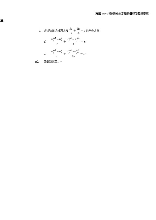
偏微分方程数值解试题(06B )参考答案与评分标准信息与计算科学专业一(10分)、设矩阵A 对称,定义)(),(),(21)(n R x x b x Ax x J ∈-=,)()(0x x J λλϕ+=.若0)0('=ϕ,则称称0x 是)(x J 的驻点(或稳定点).矩阵A 对称(不必正定),求证0x 是)(x J 的驻点的充要条件是:0x 是方程组 b Ax =的解 解: 设n R x ∈0是)(x J 的驻点,对于任意的n R x ∈,令),(2),()()()(2000x Ax x b Ax x J x x J λλλλϕ+-+=+=, (3分)0)0('=ϕ,即对于任意的n R x ∈,0),(0=-x b Ax ,特别取b Ax x -=0,则有0||||),(2000=-=--b Ax b Ax b Ax ,得到b Ax =0. (3分)反之,若n R x ∈0满足b Ax =0,则对于任意的x ,)(),(21)0()1()(00x J x Ax x x J >+==+ϕϕ,因此0x 是)(x J 的最小值点. (4分)评分标准:)(λϕ的展开式3分, 每问3分,推理逻辑性1分二(10分)、 对于两点边值问题:⎪⎩⎪⎨⎧==∈=+-=0)(,0)(),()('b u a u b a x f qu dx du p dx d Lu 其中]),([,0]),,([,0)(min )(]),,([0min ],[1b a H f q b a C q p x p x p b a C p b a x ∈≥∈>=≥∈∈建立与上述两点边值问题等价的变分问题的两种形式:求泛函极小的Ritz 形式和Galerkin 形式的变分方程。
解: 设}0)(),,(|{11=∈=a u b a H u u H E为求解函数空间,检验函数空间.取),(1b a H v E ∈,乘方程两端,积分应用分部积分得到 (3分))().(),(v f fvdx dx quv dxdv dx du p v u a b a ba ==+=⎰⎰,),(1b a H v E ∈∀ 即变分问题的Galerkin 形式. (3分)令⎰-+=-=b a dx fu qu dxdu p u f u u a u J ])([21),(),(21)(22,则变分问题的Ritz 形式为求),(1*b a H u E ∈,使)(m in )(1*u J u J EH u ∈= (4分) 评分标准:空间描述与积分步骤3分,变分方程3分,极小函数及其变分问题4分,三(20分)、对于边值问题⎪⎩⎪⎨⎧-====⨯=∈=∂∂+∂∂====x u u u u G y x y u x u y y x x 1||,0|,1|)1,0()1,0(),(,010102222 (1)建立该边值问题的五点差分格式(五点棱形格式又称正五点格式),推导截断误差的阶。
第6章_偏微分方程数值解法(附录)
第6章附录6.1 对流方程例题6.1.2计算程序!ADVECT.F!!!! advect - Program to solve the advection equation! using the various hyperbolic PDE schemesprogram advectinteger*4 MAXN, MAXnplotsparameter( MAXN = 500, MAXnplots = 500 )integer*4 method, N, nStep, i, j, ip(MAXN), im(MAXN)integer*4 iplot, nplots, iStepreal*8 L, h, c, tau, coeff, coefflw, pi, sigma, k_wavereal*8 x(MAXN), a(MAXN), a_new(MAXN), plotStepreal*8 aplot(MAXN,MAXnplots+1), tplot(MAXnplots+1)!* Select numerical parameters (time step, grid spacing, etc.).write(*,*) 'Choose a numerical method: 'write(*,*) ' 1) FTCS, 2) Lax, 3) Lax-Wendroff : 'read(*,*) methodwrite(*,*) 'Enter number of grid points: 100'read(*,*) NL = 1. ! System sizeh = L/N ! Grid spacingc = 1 ! Wave speedwrite(*,*) 'Time for wave to move one grid spacing is ', h/cwrite(*,*) 'Enter time step: 0.001'read(*,*) taucoeff = -c*tau/(2.*h) ! Coefficient used by all schemescoefflw = 2*coeff*coeff ! Coefficient used by L-W schemewrite(*,*) 'Wave circles system in ', L/(c*tau), ' steps'write(*,*) 'Enter number of steps: 300'read(*,*) nStep!* Set initial and boundary conditions.pi = 3.141592654sigma = 0.1 ! Width of the Gaussian pulsek_wave = pi/sigma ! Wave number of the cosinedo i=1,Nx(i) = (i-0.5)*h - L/2 ! Coordinates of grid pointsa(i) = cos(k_wave*x(i)) * exp(-x(i)**2/(2*sigma**2))enddo! Use periodic boundary conditionsdo i=2,(N-1)ip(i) = i+1 ! ip(i) = i+1 with periodic b.c.im(i) = i-1 ! im(i) = i-1 with periodic b.c.enddoip(1) = 2ip(N) = 1im(1) = Nim(N) = N-1!* Initialize plotting variables.iplot = 1 ! Plot counternplots = 50 ! Desired number of plotsplotStep = float(nStep)/nplotstplot(1) = 0 ! Record the initial time (t=0)do i=1,Naplot(i,1) = a(i) ! Record the initial stateenddo!* Loop over desired number of steps.do iStep=1,nStep!* Compute new values of wave amplitude using FTCS,! Lax or Lax-Wendroff method.if( method .eq. 1 ) then !!! FTCS method !!!do i=1,Na_new(i) = a(i) + coeff*( a(ip(i))-a(im(i)) )enddoelse if( method .eq. 2 ) then !!! Lax method !!!do i=1,Na_new(i) = 0.5*( a(ip(i))+a(im(i)) ) +& coeff*( a(ip(i))-a(im(i)) )enddoelse !!! Lax-Wendroff method !!!do i=1,Na_new(i) = a(i) + coeff*( a(ip(i))-a(im(i)) ) +& coefflw*( a(ip(i))+a(im(i))-2*a(i) ) enddoendifa(i) = a_new(i) ! Reset with new amplitude valuesenddo!* Periodically record a(t) for plotting.if( (iStep-int(iStep/plotStep)*plotStep) .lt. 1 ) theniplot = iplot+1tplot(iplot) = tau*iStepdo i=1,Naplot(i,iplot) = a(i) ! Record a(i) for plotingenddowrite(*,*) iStep, ' out of ', nStep, ' steps completed'endifenddonplots = iplot ! Actual number of plots recorded!* Print out the plotting variables: x, a, tplot, aplotopen(11,file='x.txt',status='unknown')open(12,file='a.txt',status='unknown')open(13,file='tplot.txt',status='unknown')open(14,file='aplot.txt',status='unknown')do i=1,Nwrite(11,*) x(i)write(12,*) a(i)do j=1,(nplots-1)write(14,1001) aplot(i,j)enddowrite(14,*) aplot(i,nplots)enddodo i=1,nplotswrite(13,*) tplot(i)enddo1001 format(e12.6,', ',$) ! The $ suppresses the carriage return stopend!***** To plot in MATLAB; use the script below ******************** !load x.txt; load a.txt; load tplot.txt; load aplot.txt;!%* Plot the initial and final states.!figure(1); clf; % Clear figure 1 window and bring forward!plot(x,aplot(:,1),'-',x,a,'--');!legend('Initial','Final');!pause(1); % Pause 1 second between plots!%* Plot the wave amplitude versus position and time!figure(2); clf; % Clear figure 2 window and bring forward!mesh(tplot,x,aplot);!ylabel('Position'); xlabel('Time'); zlabel('Amplitude');!view([-70 50]); % Better view from this angle!****************************************************************** ================================================6.2 抛物形方程例题6.2.2计算程序!!!!dftcs.f!!!!!!!!!!! dftcs - Program to solve the diffusion equation! using the Forward Time Centered Space (FTCS) scheme.program dftcsinteger*4 MAXN, MAXnplotsparameter( MAXN = 300, MAXnplots = 500 )integer*4 N, i, j, iplot, nStep, plot_step, nplots, iStepreal*8 tau, L, h, kappa, coeff, tt(MAXN), tt_new(MAXN)real*8 xplot(MAXN), tplot(MAXnplots), ttplot(MAXN,MAXnplots)!* Initialize parameters (time step, grid spacing, etc.).write(*,*) 'Enter time step: 0.0001'read(*,*) tauwrite(*,*) 'Enter the number of grid points: 50 'read(*,*) NL = 1. ! The system extends from x=-L/2 to x=L/2h = L/(N-1) ! Grid sizekappa = 1. ! Diffusion coefficientcoeff = kappa*tau/h**2if( coeff .lt. 0.5 ) thenwrite(*,*) 'Solution is expected to be stable'elsewrite(*,*) 'WARNING: Solution is expected to be unstable'endif!* Set initial and boundary conditions.do i=1,Ntt(i) = 0.0 ! Initialize temperature to zero at all pointstt_new(i) = 0.0enddo!! The boundary conditions are tt(1) = tt(N) = 0!! End points are unchanged during iteration!* Set up loop and plot variables.iplot = 1 ! Counter used to count plotsnStep = 300 ! Maximum number of iterationsplot_step = 6 ! Number of time steps between plots nplots = nStep/plot_step + 1 ! Number of snapshots (plots)do i=1,Nxplot(i) = (i-1)*h - L/2 ! Record the x scale for plotsenddo!* Loop over the desired number of time steps.do iStep=1,nStep!* Compute new temperature using FTCS scheme.do i=2,(N-1)tt_new(i) = tt(i) + coeff*(tt(i+1) + tt(i-1) - 2*tt(i))enddodo i=2,(N-1)tt(i) = tt_new(i) ! Reset temperature to new valuesenddo!* Periodically record temperature for plotting.if( mod(iStep,plot_step) .lt. 1 ) then ! Every plot_step stepsdo i=1,N ! record tt(i) for plottingttplot(i,iplot) = tt(i)enddotplot(iplot) = iStep*tau ! Record time for plotsiplot = iplot+1endifenddonplots = iplot-1 ! Number of plots actually recorded!* Print out the plotting variables: tplot, xplot, ttplotopen(11,file='tplot.txt',status='unknown')open(12,file='xplot.txt',status='unknown')open(13,file='ttplot.txt',status='unknown')do i=1,nplotswrite(11,*) tplot(i)enddowrite(12,*) xplot(i)do j=1,(nplots-1)write(13,1001) ttplot(i,j)enddowrite(13,*) ttplot(i,nplots)enddo1001 format(e12.6,', ',$) ! The $ suppresses the carriage returnstopend!***** To plot in MATLAB; use the script below ********************!load tplot.txt; load xplot.txt; load ttplot.txt;!%* Plot temperature versus x and t as wire-mesh and contour plots.!figure(1); clf;!mesh(tplot,xplot,ttplot); % Wire-mesh surface plot!xlabel('Time'); ylabel('x'); zlabel('T(x,t)');!title('Diffusion of a delta spike');!pause(1);!figure(2); clf;!contourLevels = 0:0.5:10; contourLabels = 0:5;!cs = contour(tplot,xplot,ttplot,contourLevels); % Contour plot!clabel(cs,contourLabels); % Add labels to selected contour levels!xlabel('Time'); ylabel('x');!title('Temperature contour plot');!******************************************************************! program diffu_explicit.for! explicit methods for finite diffrencedimension T(51,51)real dx,dt,lamda,kp,Tmax,Tminopen(2,file='diffu_1.dat')dx=0.5dt=0.1kp=0.835lamda=kp*dt/dx/dxTmax=100.Tmin=0.imax=21write(*,*) 'lamda=',lamdado i=1,50do j=1,50T(i,j)=0.0do j=1,40T(1,j)=TmaxT(imax,j)=Tminend dodo j=1,40do i=2,20T(i,j+1)=T(i,j)+lamda*(T(i+1,j)-2.*T(i,j)+T(i-1,j)) end dowrite(2,222) (T(i,j),i=1,21)end do222 format(1x,21(2x,f18.10))end% diffu_explicit.mclc; clear all;nl = 20.; nt = 40;dx = 0.5; dt = 0.1; kp = 0.835;lamda = kp*dt/dx/dx;Tl = 0.; Tr = 100.;T = zeros(nl,nt);T(1,:) = Tl; T(nl,:)=Tr;for j=1:nt-1for i =2:nl-1T(i,j+1)=T(i,j)+lamda*(T(i+1,j)-2.*T(i,j)+T(i-1,j));endendsurf(T');xlabel('x');ylabel('time');zlabel('Temperature');title('explicit scheme');! diffu_implicit.for! implicit methods for finite diffrenceexternal tridparameter (imax=21,kmax=50)dimension t(imax),a(imax),b(imax),c(imax),r(imax),u(imax) real dx,dt,lamda,kp,tmax,tminopen(2,file='diffu_2.dat')dx=0.5lamda=kp*dt/dx/dxtmax=100.tmin=0.write(*,*) 'lamda=',lamdado i=2,imax-1! t(i)=tmax-(tmax-tmin)/(imax-1.)*(i-1.) t(i)=0.0end dot(1)=tmaxt(imax)=tmin! write(*,*) a(i),b(i),c(i)b(1)=1.c(1)=0.r(1)=t(1)a(imax)=0.b(imax)=1.r(imax)=t(imax)do i=2,imax-1a(i)=-lamdab(i)=1.+2.*lamdac(i)=-lamdar(i)=t(i)end dok=01 k=k+1call trid(a,b,c,r,u,imax)do i=1,imaxt(i)=u(i)r(i)=u(i)end dowrite(2,222) (t(i),i=1,imax)! write(*,222) (t(i),i=1,imax)if(k.lt.kmax) goto 1222 format(1x,21(2x,f18.12))endsubroutine trid(a,b,c,r,u,n)parameter (nmax=100)real gam(nmax),a(n),b(n),c(n),u(n),r(n)if (b(1)==0.) pause 'b(1)=0 in trid'bet=b(1)u(1)=r(1)/betdo j=2,ngam(j)=c(j-1)/betbet=b(j)-a(j)*gam(j)if (bet==0.) pause 'bet=0 in trid'u(j)=(r(j)-a(j)*u(j-1))/betend dodo j=n-1,1,-1u(j)=u(j)-gam(j+1)*u(j+1)end doend subroutine trid================================================== 6.3椭圆方程例题6.3.1计算程序! program overrelaxation.for! overrelaxation_iteration_methods for finite diffrence! of the 2d_Laplacian difference equationparameter(imax=25,jmax=25,pi=3.1415926)dimension T(imax,jmax),a(imax,jmax),& qx(imax,jmax),qy(imax,jmax),q(imax,jmax),an(imax,jmax) real lamda,Tu,Td,Tl,Tr,kpx,kpy,dx,dyopen(2,file='overrelaxation.dat')open(3,file='q.dat')lamda=1.5;Tu=100.;Tl=75.;Tr=50.;Td=0.;dx=1.;dy=1.;kmax=9 kpx=-0.49/2./dx;kpy=-0.49/2./dydo i=1,imaxdo j=1,jmaxT(i,j)=0.0end doend doT(1,1)=0.5*(Td+Tl) ;T(1,jmax)=0.5*(Tl+Tu)T(imax,jmax)=0.5*(Tu+Tr);T(imax,1)=0.5*(Tr+Td)do j=2,jmax-1T(1,j)=Tl; T(imax,j)=Trend dodo i=2, imax-1T(i,1)=Td; T(i,jmax)=Tuend dok=0do i=2,imax-1do j=2,jmax-1a(i,j)=T(i,j)T(i,j)=0.25*(T(i+1,j)+T(i-1,j)+T(i,j+1)+T(i,j-1))T(i,j)=lamda*T(i,j)+(1.-lamda)*a(i,j)end doend doep=abs((T(2,2)-a(2,2))/T(2,2))if(k.lt.kmax) goto 5write(*,*) 'ep=',epdo j=1,jmaxwrite(2,222) (T(i,j),i=1,imax)end do222 format(1x,25(2x,f14.10))do i=2,imax-1do j=2,jmax-1qx(i,j)=kpx*(T(i+1,j)-T(i-1,j))qy(i,j)=kpy*(T(i,j+1)-T(i,j-1))q(i,j)=sqrt(qx(i,j)*qx(i,j)+qy(i,j)*qy(i,j))if(qx(i,j).gt.0.) thenan(i,j)=atan(qy(i,j)/qx(i,j))elsean(i,j)=atan(qy(i,j)/qx(i,j))+piend ifend doend dodo j=2,jmax-1do i=2,imax-1! write(3,333) dx*(i-1),dy*(j-1),an(i,j),q(i,j)write(3,333) dx*(i-1),dy*(j-1),qx(i,j),qy(i,j)end doend do333 format(1x,4(2x,f18.12))End================================================= 例题6.3.2计算程序!!!!xadi.f90!!!!!program xadiuse AVDefuse DFLibparameter(n=19)real aj(n),bj(n),cj(n)integer statusreal T(0:n,0:n),TT(0:n,0:n)real lamda,Tu,Td,Tl,Tr,dx,dy,dt,kaopen(2,file='T3.dat')Tu=100.;Tl=75.;Tr=50.;Td=0.;dx=1.;dy=1.;kmax=10;dt=1.ka=0.835; lamda=ka*dt/(dx*dx)write(*,*) 'lamda=',lamdaT = 0.T(0,:) = Tl; T(n,:) =TrT(:,0) = Td; T(:,n) =TuT(0,0)=0.5*(Td+Tl);T(0,n)=0.5*(Tl+Tu)T(n,n)=0.5*(Tu+Tr);T(n,0)=0.5*(Tr+Td)! 系数矩阵赋值aj(:)=-lamda; ai(:)=lamdabj(:)= 2.*(1.+lamda); bi(:)=2.*(1-lamda)cj(:)=-lamda; ci(:)=lamdacall faglStartWatch(T, status)! 相当于随时间演化do k=1,kmaxdo i=1,n-1do j=1,n-1r(j)=ai(i)*T(i-1,j)+bi(i)*T(i,j)+ci(i)*T(i+1,j)end dor(1)=r(1)-aj(1)*T(i,0)r(n-1)=r(n-1)-cj(n-1)*T(i,n)call tridag(aj,bj,cj,r,u,n-1)do j=1,n-1T(i,j)=u(j)end doend do! 将矩阵T转置计算x方向call reverse(n,T,TT)do i=1,n-1do j=1,n-1r(j)=ai(i)*TT(i-1,j)+bi(i)*TT(i,j)+ci(i)*TT(i+1,j) end dor(1)=r(1)-aj(1)*TT(i,0)r(n-1)=r(n-1)-cj(n-1)*TT(i,n)call tridag(aj,bj,cj,r,u,n-1)do j=1,n-1TT(i,j)=u(j)end doend docall reverse(n,TT,T)call faglUpdate(T, status)call faglShow(T, status)end dopausecall faglClose(T, status)call faglEndWatch(T, status)do j=0,nwrite(2,222) (T(i,j),i=0,n)end do222 format(1x,20(2x,f14.10))endSUBROUTINE tridag(a,b,c,r,u,n)INTEGER n,NMAXREAL a(n),b(n),c(n),r(n),u(n)PARAMETER (NMAX=500)INTEGER jREAL bet,gam(NMAX)if(b(1).eq.0.)pause 'tridag: rewrite equations'bet=b(1)u(1)=r(1)/betdo 11 j=2,ngam(j)=c(j-1)/betbet=b(j)-a(j)*gam(j)if(bet.eq.0.)pause 'tridag failed'u(j)=(r(j)-a(j)*u(j-1))/bet11 continuedo 12 j=n-1,1,-1u(j)=u(j)-gam(j+1)*u(j+1)12 continuereturnENDSUBROUTINE REVERSE(n,T,TT) integer n,i,jreal T(0:n,0:n),TT(0:n,0:n)do i=0,ndo j=0,nTT(i,j)=T(j,i)end doend doreturnend================================================6.4 非线性偏微分方程% gasdynamincs_lw_1.mclc; clear all;xmin=-1.; xmax=1.; nx=101; h=(xmax-xmin)/(nx-1);r=0.9; cad=0.; time=0.; gamma=1.4; bcl=1.; bcr=1.;fprintf(' Space step - %f \n',h); fprintf(' \n');dd(1:nx)=zeros(1,nx); ud(1:nx)=zeros(1,nx); pd(1:nx)=zeros(1,nx);x(1:nx)=xmin+((1:nx)-1)*h;% Test 1te=' ( Test 1 )';rol=1.; ul=0.; pl=1.;ror=0.125; ur=0.; pr=0.1;tp=5.5;% Test 3%te=' ( Test 3 )';%rol=0.1; ul=0.; pl=1.;%ror=1.; ur=0.; pr=100.;%tp=0.05;% Initial conditionsdd(1:(nx-1)/2+1)=rol; ud(1:(nx-1)/2+1)=ul; pd(1:(nx-1)/2+1)=pl;dd((nx-1)/2+2:nx)=ror;ud((nx-1)/2+2:nx)=ur; pd((nx-1)/2+2:nx)=pr;[d,u,p,e,time]=lw_gasdynamics(dd,ud,pd,h,nx,r,cad,tp,gamma,bcl,bcr);% Exact solutionfor n=1:nx[density, velocity, pressure]=riemann(x(n),time,rol,ul,pl,ror,ur,pr,gamma);de(n)=density; ue(n)=velocity; pe(n)=pressure;ee(n)=pressure/((gamma-1.)*density);endfigure(1);plot(x,de,'k-',x,d,'k--');xlabel(' x ');ylabel(' density ');title([' Example 6.1 ',te]);figure(2);plot(x,ue,'k-',x,u,'k--');xlabel(' x ');ylabel(' velocity ');title([' Example 6.1 ',te]);figure(3);plot(x,pe,'k-',x,p,'k--');xlabel(' x ');ylabel(' pressure ');title([' Example 6.1 ',te]);figure(4);plot(x,ee,'k-',x,e,'k--');xlabel(' x ');ylabel(' internal energy ');title([' Example 6.1 ',te]);clear all;% Lax-Wendroff scheme (gasdynamics)function [d,u,p,e,time]=lw_gasdynamics(dd,ud,pd,h,nx,r,cad,tp,gamma,bcl,bcr)sd(1,1:nx)=dd(1:nx);sd(2,1:nx)=dd(1:nx).*ud(1:nx);sd(3,1:nx)=pd(1:nx)/(gamma-1.)+0.5*(dd(1:nx).*ud(1:nx)).*ud(1:nx);si(1:3,1:nx+1)=zeros(3,nx+1); av(1:3,1:nx)=zeros(3,nx);time=0.;while time <= tpsta=max(abs(sd(2,:)./sd(1,:))+...sqrt(gamma*(gamma-1)*(sd(3,:)./sd(1,:)-0.5*(sd(2,:).*sd(2,:))./(sd(1,:).*sd(1,:)))));tau=r*h*sqrt(1.-2.*cad)/sta;time=time+tau; %fprintf(' time - %f \n',time);% first stepif bcl == 0sl1=sd(1,2); sl2=-sd(2,2); sl3=sd(3,2);elsesl1=sd(1,2); sl2=sd(2,2); sl3=sd(3,2);endgl(1)=sl2;gl(2)=(gamma-1.)*sl3+0.5*(3.-gamma)*sl2^2/sl1;gl(3)=sl2*(gamma*sl3-0.5*(gamma-1.)*sl2^2/sl1)/sl1;for n=1:nxif (n == 1)|(n == nx)av(:,n)=[ 0.; 0.; 0.;];elseav(:,n)=cad*(sd(:,n+1)-2.*sd(:,n)+sd(:,n-1));endsr1=sd(1,n); sr2=sd(2,n); sr3=sd(3,n);gr(1)=sr2;gr(2)=(gamma-1.)*sr3+0.5*(3.-gamma)*sr2^2/sr1;gr(3)=sr2*(gamma*sr3-0.5*(gamma-1.)*sr2^2/sr1)/sr1;si(1,n)=0.5*(sl1+sr1)-(gr(1)-gl(1))*tau*0.5/h;si(2,n)=0.5*(sl2+sr2)-(gr(2)-gl(2))*tau*0.5/h;si(3,n)=0.5*(sl3+sr3)-(gr(3)-gl(3))*tau*0.5/h;gl(:)=gr(:);sl1=sr1; sl2=sr2; sl3=sr3;endif bcr == 0sr1=sd(1,nx-1); sr2=-sd(2,nx-1); sr3=sd(3,nx-1);elsesr1=sd(1,nx-1); sr2=sd(2,nx-1); sr3=sd(3,nx-1);endgr(1)=sr2;gr(2)=(gamma-1.)*sr3+0.5*(3.-gamma)*sr2^2/sr1;gr(3)=sr2*(gamma*sr3-0.5*(gamma-1.)*sr2^2/sr1)/sr1;si(1,nx+1)=0.5*(sl1+sr1)-(gr(1)-gl(1))*tau*0.5/h;si(2,nx+1)=0.5*(sl2+sr2)-(gr(2)-gl(2))*tau*0.5/h;si(3,nx+1)=0.5*(sl3+sr3)-(gr(3)-gl(3))*tau*0.5/h;% second stepfl(1)=si(2,1);fl(2)=(gamma-1.)*si(3,1)+0.5*(3.-gamma)*si(2,1)^2/si(1,1);fl(3)=si(2,1)*(gamma*si(3,1)-0.5*(gamma-1.)*si(2,1)^2/si(1,1))/si(1,1);for n=2:nx+1fr(1)=si(2,n);fr(2)=(gamma-1.)*si(3,n)+0.5*(3.-gamma)*si(2,n)^2/si(1,n);fr(3)=si(2,n)*(gamma*si(3,n)-0.5*(gamma-1.)*si(2,n)^2/si(1,n))/si(1,n);su(:,n-1)=sd(:,n-1)-(fr(:)-fl(:))*tau/h+av(:,n-1);fl(:)=fr(:);endsd(:,1:nx)=su(:,1:nx);endd(1:nx)=su(1,1:nx); u(1:nx)=su(2,1:nx)./su(1,1:nx);p(1:nx)=(gamma-1.)*(su(3,1:nx)-0.5*(su(2,1:nx).*su(2,1:nx))./su(1,1:nx));e(1:nx)=(su(3,1:nx)-0.5*(su(2,1:nx).*su(2,1:nx))./su(1,1:nx))./su(1,1:nx);return;% Solves Riemann problem for ideal gas% r1, u1, p1 initial parameters for x<0% r2, u2, p2 initial parameters for x>0% rf, uf, pf solution at the point (x,t)% c1, c2 sound speeds for x<0 and for x>0% s1, sr velocties of the fronts of S(hock)W(ave)s% shl, shr velocties of the fronts of the heads of R(arefaction)Ws% stl, str velocties of the tails of RWsfunction [rf,uf,pf]=riemann(x,t,r1,u1,p1,r2,u2,p2,gamma)g(1)=0.5*(gamma-1.)/gamma; g(2)=0.5*(gamma+1.)/gamma; g(3)=2.*gamma/(gamma-1.); g(4)=2./(gamma-1.); g(5)=2./(gamma+1.); g(6)=(gamma-1.)/(gamma+1.);g(7)=0.5*(gamma-1.); g(8)=1./gamma; g(9)=gamma-1.;s=x/t;c1 = sqrt(p1/(r1*g(8)));c2 = sqrt(p2/(r2*g(8)));du=u2-u1;% Vacuum solutionuvac=g(4)*(c1+c2)-du;if uvac <= 0.disp(' Vacuum generated by given data');return;end% Apply Newton method% Initial guessespv=0.5*(p1+p2)-0.125*du*(r1+r2)*(c1+c2);pmin=min(p1,p2); pmax=max(p1,p2); qrat=pmax/pmin;if ( qrat <= 2. ) & ( pmin <= pv & pv <= pmax )p=max(1.0e-6,pv);elseif pv < pminpnu=c1+c2-g(7)*du;pde=c1/(p1^g(1))+c2/(p2^g(1));p=(pnu/pde)^g(3);elsegel=sqrt((g(5)/r1)/(g(6)*p1+max(1.0e-6,pv)));ger=sqrt((g(5)/r2)/(g(6)*p2+max(1.0e-6,pv)));p=(gel*p1+ger*p2-du)/(gel+ger); p=max(1.0e-6,p);endendp0=p; err=1.;while err > 1.0e-5if p <= p1prat=p/p1; fl=g(4)*c1*(prat^g(1)-1.); ffl=1./(r1*c1*prat^g(2));elsea=g(5)/r1; b=g(6)*p1; qrt=sqrt(a/(b+p));fl=(p-p1)*qrt; ffl=(1.-0.5*(p-p1)/(b+p))*qrt;endif p <= p2prat=p/p2; fr=g(4)*c2*(prat^g(1)-1.); ffr=1./(r2*c2*prat^g(2));elsea=g(5)/r2; b=g(6)*p2; qrt=sqrt(a/(b+p));fr=(p-p2)*qrt; ffr=(1.-0.5*(p-p2)/(b+p))*qrt;endp=p-(fl+fr+du)/(ffl+ffr);err=2.*abs(p-p0)/(p+p0); p0=p;endif p0 < 0.p0=1.0e-6;end% Velocity of CDu0=0.5*(u1+u2+fr-fl);if s <= u0if p0 <= p1shl=u1-c1;if s <= shlrf=r1; uf=u1; pf=p1; return;elsecml=c1*(p0/p1)^g(1); stl=u0-cml;if s > stlrf=r1*(p0/p1)^g(8); uf=u0; pf=p0; return;elseuf=g(5)*(c1+g(7)*u1+s); c=g(5)*(c1+g(7)*(u1-s));rf=r1*(c/c1)^g(4); pf=p1*(c/c1)^g(3);return;endendelsepml=p0/p1; sl=u1-c1*sqrt(g(2)*pml+g(1));if s <= slrf=r1; uf=u1; pf=p1; return;elserf=r1*(pml+g(6))/(pml*g(6)+1.); uf=u0; pf=p0; return;endendelseif p0 > p2pmr=p0/p2; sr=u2+c2*sqrt(g(2)*pmr+g(1));if s >= srrf=r2; uf=u2; pf=p2; return;elserf=r2*(pmr+g(6))/(pmr*g(6)+1.); uf=u0; pf=p0; return;endelseshr=u2+c2;if s >= shrrf=r2; uf=u2; pf=p2; return;elsecmr=c2*(p0/p2)^g(1); str=u0+cmr;if s <= strrf=r2*(p0/p2)^g(8); uf=u0; pf=p0; return;elseuf=g(5)*(-c2+g(7)*u2+s); c=g(5)*(c2-g(7)*(u2-s));rf=r2*(c/c2)^g(4); pf=p2*(c/c2)^g(3);return;endendendendreturn;%%%%%%%%% gasdynamics_Godunov.m%%%%%%%%%%%%%clc; clear all;xmin=-1.; xmax=1.; nx=101; h=(xmax-xmin)/(nx-1);r=0.9; gamma=1.4; bcl=1.; bcr=1.;fprintf('gasdynamics_godunov \n'); fprintf(' Space step - %f \n',h); fprintf(' \n'); dd(1:nx-1)=zeros(1,nx-1); ud(1:nx-1)=zeros(1,nx-1); pd(1:nx-1)=zeros(1,nx-1);x(1:nx)=xmin+((1:nx)-1)*h; xa=xmin+((1:nx-1)-0.5)*h;% Test 1te=' ( Test 1 )';rol=1.; ul=0.; pl=1.;ror=0.125; ur=0.; pr=0.1;tp=15.5;% Test 2%te=' ( Test 2 )';%rol=1.; ul=0.; pl=1000.;%ror=1.; ur=0.; pr=1.;%tp=0.024;% Test 3%te=' ( Test 3 )';%rol=0.1; ul=0.; pl=1.;%ror=1.; ur=0.; pr=100.;%tp=0.05;% Test 4%te=' ( Test 4 )';%rol=5.99924; ul=19.5975; pl=460.894;%ror=5.99242; ur=-6.19633; pr=46.0950;%tp=0.05;% Test 5%te=' ( Test 5 )';%rol=3.86; ul=-0.81; pl=10.33;%ror=1.; ur=-3.44; pr=1.;%tp=0.5;% Initial conditionsdd(1:(nx-1)/2)=rol; ud(1:(nx-1)/2)=ul; pd(1:(nx-1)/2)=pl;dd((nx-1)/2+1:nx-1)=ror;ud((nx-1)/2+1:nx-1)=ur; pd((nx-1)/2+1:nx-1)=pr;[d,u,p,e,time]=godunov_gasdynamics(dd,ud,pd,h,nx,r,tp,gamma,bcl,bcr);% Exact solutionfor n=1:nx[density, velocity, pressure]=riemann(x(n),time,rol,ul,pl,ror,ur,pr,gamma);de(n)=density; ue(n)=velocity; pe(n)=pressure;ee(n)=pressure/((gamma-1.)*density);endfigure(1);plot(x,de,'k-',xa,d,'ko');xlabel(' x ');ylabel(' density ');title([' Example 6.3 ',te]);figure(2);plot(x,ue,'k-',xa,u,'ko');xlabel(' x ');ylabel(' velocity ');figure(3);plot(x,pe,'k-',xa,p,'ko');xlabel(' x ');ylabel(' pressure ');figure(4);plot(x,ee,'k-',xa,e,'ko');xlabel(' x ');ylabel(' internal energy ');clear all;% Method of S. K. Godunovfunction [d,u,p,e,time]=godunov_gasdynamics(dd,ud,pd,h,nx,r,tp,gamma,bcl,bcr)g(1)=0.5*(gamma-1.)/gamma; g(2)=0.5*(gamma+1.)/gamma; g(3)=2.*gamma/(gamma-1.); g(4)=2./(gamma-1.); g(5)=2./(gamma+1.); g(6)=(gamma-1.)/(gamma+1.);g(7)=0.5*(gamma-1.); g(8)=1./gamma; g(9)=gamma-1.;sd(1,1:nx-1)=dd(1:nx-1);sd(2,1:nx-1)=dd(1:nx-1).*ud(1:nx-1);sd(3,1:nx-1)=pd(1:nx-1)/(gamma-1.)+0.5*(dd(1:nx-1).*ud(1:nx-1)).*ud(1:nx-1);time=0.;while time <= tpsta=max(abs(sd(2,:)./sd(1,:))+...sqrt(gamma*(gamma-1)*(sd(3,:)./sd(1,:)-0.5*(sd(2,:).*sd(2,:))./(sd(1,:).*sd(1,:)))));tau=r*h/sta;time=time+tau; %fprintf(' %f \n',time);if bcl == 0[f1,f2,f3]=flux_godunov(sd(1,1),-sd(2,1),sd(3,1),sd(1,1),sd(2,1),sd(3,1),g(:));else[f1,f2,f3]=flux_godunov(sd(1,1),sd(2,1),sd(3,1),sd(1,1),sd(2,1),sd(3,1),g(:));endfleft(1)=f1; fleft(2)=f2; fleft(3)=f3;for n=1:nx-2[f1,f2,f3]=flux_godunov(sd(1,n),sd(2,n),sd(3,n),sd(1,n+1),sd(2,n+1),sd(3,n+1),g(:));fright(1)=f1; fright(2)=f2; fright(3)=f3;su(:,n)=sd(:,n)-(fright(:)-fleft(:))*tau/h;fleft(:)=fright(:);endif bcr == 0[f1,f2,f3]=flux_godunov(sd(1,nx-1),sd(2,nx-1),sd(3,nx-1),sd(1,nx-1),-sd(2,nx-1),...sd(3,nx-1),g(:));else[f1,f2,f3]=flux_godunov(sd(1,nx-1),sd(2,nx-1),sd(3,nx-1),sd(1,nx-1),sd(2,nx-1),...sd(3,nx-1),g(:));endfright(1)=f1; fright(2)=f2; fright(3)=f3;su(:,nx-1)=sd(:,nx-1)-(fright(:)-fleft(:))*tau/h;sd(:,1:nx-1)=su(:,1:nx-1);endd(1:nx-1)=su(1,1:nx-1); u(1:nx-1)=su(2,1:nx-1)./su(1,1:nx-1);p(1:nx-1)=(gamma-1.)*(su(3,1:nx-1)-0.5*(su(2,1:nx-1).*su(2,1:nx-1))./su(1,1:nx-1));e(1:nx-1)=(su(3,1:nx-1)-0.5*(su(2,1:nx-1).*su(2,1:nx-1))./su(1,1:nx-1))./su(1,1:nx-1); return;% Solves Riemann problem for ideal gas% r1, u1, p1 initial parameters for x<0% r2, u2, p2 initial parameters for x>0% rf, uf, pf solution at the point (x,t)% c1, c2 sound speeds for x<0 and for x>0% s1, sr velocties of the fronts of S(hock)W(ave)s% shl, shr velocties of the fronts of the heads of R(arefaction)Ws% stl, str velocties of the tails of RWsfunction [rf,uf,pf]=riemann(x,t,r1,u1,p1,r2,u2,p2,gamma)g(1)=0.5*(gamma-1.)/gamma; g(2)=0.5*(gamma+1.)/gamma; g(3)=2.*gamma/(gamma-1.);g(7)=0.5*(gamma-1.); g(8)=1./gamma; g(9)=gamma-1.;s=x/t;c1 = sqrt(p1/(r1*g(8)));c2 = sqrt(p2/(r2*g(8)));du=u2-u1;% Vacuum solutionuvac=g(4)*(c1+c2)-du;if uvac <= 0.disp(' Vacuum generated by given data');return;end% Apply Newton method% Initial guessespv=0.5*(p1+p2)-0.125*du*(r1+r2)*(c1+c2);pmin=min(p1,p2); pmax=max(p1,p2); qrat=pmax/pmin;if ( qrat <= 2. ) & ( pmin <= pv & pv <= pmax )p=max(1.0e-6,pv);elseif pv < pminpnu=c1+c2-g(7)*du;pde=c1/(p1^g(1))+c2/(p2^g(1));p=(pnu/pde)^g(3);elsegel=sqrt((g(5)/r1)/(g(6)*p1+max(1.0e-6,pv)));ger=sqrt((g(5)/r2)/(g(6)*p2+max(1.0e-6,pv)));p=(gel*p1+ger*p2-du)/(gel+ger); p=max(1.0e-6,p);endendp0=p; err=1.;while err > 1.0e-5if p <= p1prat=p/p1; fl=g(4)*c1*(prat^g(1)-1.); ffl=1./(r1*c1*prat^g(2));elsea=g(5)/r1; b=g(6)*p1; qrt=sqrt(a/(b+p));fl=(p-p1)*qrt; ffl=(1.-0.5*(p-p1)/(b+p))*qrt;endif p <= p2prat=p/p2; fr=g(4)*c2*(prat^g(1)-1.); ffr=1./(r2*c2*prat^g(2));a=g(5)/r2; b=g(6)*p2; qrt=sqrt(a/(b+p));fr=(p-p2)*qrt; ffr=(1.-0.5*(p-p2)/(b+p))*qrt;endp=p-(fl+fr+du)/(ffl+ffr);err=2.*abs(p-p0)/(p+p0); p0=p;endif p0 < 0.p0=1.0e-6;end% Velocity of CDu0=0.5*(u1+u2+fr-fl);if s <= u0if p0 <= p1shl=u1-c1;if s <= shlrf=r1; uf=u1; pf=p1; return;elsecml=c1*(p0/p1)^g(1); stl=u0-cml;if s > stlrf=r1*(p0/p1)^g(8); uf=u0; pf=p0; return;elseuf=g(5)*(c1+g(7)*u1+s); c=g(5)*(c1+g(7)*(u1-s));rf=r1*(c/c1)^g(4); pf=p1*(c/c1)^g(3);return;endendelsepml=p0/p1; sl=u1-c1*sqrt(g(2)*pml+g(1));if s <= slrf=r1; uf=u1; pf=p1; return;elserf=r1*(pml+g(6))/(pml*g(6)+1.); uf=u0; pf=p0; return;endendelseif p0 > p2pmr=p0/p2; sr=u2+c2*sqrt(g(2)*pmr+g(1));if s >= srrf=r2; uf=u2; pf=p2; return;rf=r2*(pmr+g(6))/(pmr*g(6)+1.); uf=u0; pf=p0; return;endelseshr=u2+c2;if s >= shrrf=r2; uf=u2; pf=p2; return;elsecmr=c2*(p0/p2)^g(1); str=u0+cmr;if s <= strrf=r2*(p0/p2)^g(8); uf=u0; pf=p0; return;elseuf=g(5)*(-c2+g(7)*u2+s); c=g(5)*(c2-g(7)*(u2-s));rf=r2*(c/c2)^g(4); pf=p2*(c/c2)^g(3);return;endendendendreturn;% Solves Riemann problem and computes fluxes for method of S. K. Godunov% r1, u1, p1 parameters in left cell% r2, u2, p2 parameters in right cell% rf, uf, pf parameters on the interface% c1, c2 sound speeds in left and right cells% s1, sr velocties of the fronts of S(hock)W(ave)s% shl, shr velocties of the fronts of the heads of R(arefaction)Ws% stl, str velocties of the tails of RWsfunction [f1,f2,f3]=flux_godunov(sl1,sl2,sl3,sr1,sr2,sr3,g)r1=sl1; u1=sl2/r1; p1=(1./g(8)-1.)*(sl3-0.5*sl2*u1);r2=sr1; u2=sr2/r2; p2=(1./g(8)-1.)*(sr3-0.5*sr2*u2);% sound speeds in left and right cellsc1 = sqrt(p1/(r1*g(8)));c2 = sqrt(p2/(r2*g(8)));du=u2-u1;% Vacuum solution。
偏微分方程数值解法试题与答案
一.填空(1553=⨯分)1.若步长趋于零时,差分方程的截断误差0→lmR ,则差分方程的解lm U 趋近于微分方程的解lm u . 此结论_______(错或对); 2.一阶Sobolev 空间{})(,,),()(21Ω∈''=ΩL f f f y x f H y x关于内积=1),(g f _____________________是Hilbert 空间;3.对非线性(变系数)差分格式,常用 _______系数法讨论差分格式的_______稳定性; 4.写出3x y =在区间]2,1[上的两个一阶广义导数:_________________________________, ________________________________________;5.隐式差分格式关于初值是无条件稳定的. 此结论_______(错或对)。
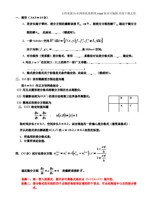
二.(13分)设有椭圆型方程边值问题用1.0=h 作正方形网格剖分 。
(1)用五点菱形差分格式将微分方程在内点离散化; (2)用截断误差为)(2h O 的差分法将第三边界条件离散化; (3)整理后的差分方程组为 三.(12)给定初值问题xut u ∂∂=∂∂ , ()10,+=x x u 取时间步长1.0=τ,空间步长2.0=h 。
试合理选用一阶偏心差分格式(最简显格式), 并以此格式求出解函数),(t x u 在2.0,2.0=-=t x 处的近似值。
1.所选用的差分格式是: 2.计算所求近似值:四.(12分)试讨论差分方程()ha h a r u u r u u k l k l k l k l ττ+-=-+=++++11,1111逼近微分方程0=∂∂+∂∂xu a t u 的截断误差阶R 。
思路一:将r 带入到原式,展开后可得格式是在点(l+1/2,k+1/2)展开的。
思路二:差分格式的用到的四个点刚好是矩形区域的四个顶点,可由此构造中心点的差分格式。
偏微分方程数值解试题参考答案
偏微分方程数值解一(10分)、设矩阵A 对称正定,定义)(),(),(21)(n R x x b x Ax x J ∈-=,证明下列两个问题等价:(1)求n R x ∈0使)(min )(0x J x J n Rx ∈=;(2)求下列方程组的解:b Ax = 解: 设n R x ∈0是)(x J 的最小值点,对于任意的n R x ∈,令),(2),()()()(2000x Ax x b Ax x J x x J λλλλϕ+-+=+=, (3分)因此0=λ是)(λϕ的极小值点,0)0('=ϕ,即对于任意的n R x ∈,0),(0=-x b Ax ,特别取b Ax x -=0,则有0||||),(2000=-=--b Ax b Ax b Ax ,得到b Ax =0. (3分) 反之,若nR x ∈0满足bAx =0,则对于任意的x ,)(),(21)0()1()(00x J x Ax x x J >+==+ϕϕ,因此0x 是)(x J 的最小值点. (4分)评分标准:)(λϕ的表示式3分, 每问3分,推理逻辑性1分二(10分)、对于两点边值问题:⎪⎩⎪⎨⎧==∈=+-=0)(,0)(),()(b u a u b a x f qu dxdu p dx d Lu 其中]),([,0]),,([,0)(min )(]),,([0min ],[1b a H f q b a C q p x p x p b a C p b a x ∈≥∈>=≥∈∈建立与上述两点边值问题等价的变分问题的两种形式:求泛函极小的Ritz 形式和Galerkin 形式的变分方程。
解: 设}0)()(),,(|{11==∈=b u a u b a H u u H 为求解函数空间,检验函数空间.取),(10b a H v ∈,乘方程两端,积分应用分部积分得到 (3分))().(),(v f fvdx dx quv dxdv dx du p v u a b a ba ==+=⎰⎰,),(1b a H v ∈∀ 即变分问题的Galerkin 形式. (3分)令⎰-+=-=b a dx fu qu dxdup u f u u a u J ])([21),(),(21)(22,则变分问题的Ritz 形式为求),(1*b a H u ∈,使)(m in )(10*u J u J H u ∈= (4分) 评分标准:空间描述与积分步骤3分,变分方程3分,极小函数及其变分问题4分,三(20分)、对于边值问题⎪⎩⎪⎨⎧=⨯=∈-=∂∂+∂∂∂0|)1,0()1,0(),(,12222G u G y x yux u (1)建立该边值问题的五点差分格式(五点棱形格式又称正五点格式),推导截断误差的阶。
(完整word版)偏微分方程数值解习题解答案
(完整 word 版)偏微分方程数值解习题解答案 a6
(完整 word 版)偏微分方程数值解习题解答案 q7
a7 q8
(完整 word 版)偏微分方程数值解习题解答案 a8
(完整 word 版)偏微分方程数值解习题解答案 q9
q10
(完整 word 版)偏微分方程数值解习题解答案
(完整 word 版)偏微分方程数值解习题解答案 q11
a1 q2
(完整 word 版)偏微分方程数值解习题解答案
(完整 word 版)偏微分方程数值解习题解答案 q3
(完整 word 版)偏微分方程数值解习题解答案
(完整 word 版)偏微分方程数值解习题解答案 q4
(完整 word 版)偏微分方程数值解习题解答案
(完整 word 版)偏微分方程数值解习题解答案 q5
(完整 word 版)偏微分方程数值解习题解答案 q3
(完整 word 版)偏微分方程数值解习题解答案
(完整 word 版)偏微分方程数值解习题解答案 q4
(完整 word 版)偏微分方程数值解习题解答案
(完整 word 版)偏微分方程数值解习题解答案 q5
a5
(完整 word 版)偏微分方程数值解习题解答案 q6
(完整 word 版)偏微分方程数值解习题解答案
(完整 word 版)偏微分方程数值解习题解答案 q12
a12 第二章 第三章 第四章 第五章 第六章 q1
(完整 word 版)偏微分方程数值解习题解答案 1
(完整 word 版)偏微分方程数值解习题解答案
2 q3
(完整 word 版)偏微分方程数值解习题解答案 a3
六章 q1
(完整 word 版)偏微分方程数值解习题解答案
数学偏微分方程的数值解法
数学偏微分方程的数值解法当然可以。
这里是根据标题“数学偏微分方程的数值解法”出的20道试题,包括选择题和填空题,每道题目都有详细的序号介绍:1. 选择题:偏微分方程的数值解法主要适用于哪类方程?A. 常微分方程B. 偏微分方程C. 代数方程D. 差分方程2.填空题:数值解法中常用的一种基础方法是______________。
3.选择题:有限差分法是一种适用于哪种类型的偏微分方程的数值解法?A. 椭圆型B. 抛物型C. 双曲型D. 超越型4.填空题:偏微分方程的数值解法通常要求将空间区域离散化为___ ___________。
5. 选择题:哪种方法适合处理偏微分方程的初始值问题?A. 有限元法B. 有限差分法C. 傅里叶变换法D. 辛普森法则6.填空题:数值解法中,常用的稳定性分析方法包括_____________ _。
7.选择题:对于偏微分方程的边值问题,常用的数值方法是_______ _______。
A. 有限体积法B. 辛普森法则C. 椭圆积分法D. 有限元法8.填空题:描述一种常见的数值解法的收敛性条件______________。
9.选择题:哪种方法在处理时间依赖性偏微分方程时特别有效?A. 隐式方法B. 显式方法C. 中心差分法D. 前进差分法10.填空题:数值解法中的矩阵求解通常利用______________方法。
11.选择题:在有限元法中,通常要对空间区域进行如何划分?A. 正交分解B. 三角剖分C. 曲面划分D. 直角分割12.填空题:有限差分法的精度通常与______________相关。
13.选择题:哪种方法适合处理非线性偏微分方程的数值解?A. 变分法B. 有限元法C. 辛普森法则D. 显式方法14.填空题:对于稳定性的要求,常用的数值方法需要满足_________ _____条件。
15.选择题:哪种方法可以有效地处理多维偏微分方程的数值解?A. 傅里叶变换法B. 辛普森法则C. 多重网格法D. 变分法16.填空题:在求解偏微分方程数值解时,通常需要考虑___________ ___问题。
偏微分方程数值解期末试题及参考答案
《偏微分方程数值解》试卷参考答案与评分标准专业班级信息与计算科学开课系室考试日期 2006.4.14命题教师王子亭偏微分方程数值解试题(06A)参考答案与评分标准信息与计算科学专业一(10分)、设矩阵A 对称正定,定义)(),(),(21)(n R x x b x Ax x J ∈-=,证明下列两个问题等价:(1)求n R x ∈0使 )(min )(0x J x J nRx ∈=;(2)求下列方程组的解:b Ax =解: 设n R x ∈0是)(x J 的最小值点,对于任意的n R x ∈,令),(2),()()()(2000x Ax x b Ax x J x x J λλλλϕ+-+=+=, (3分)因此0=λ是)(λϕ的极小值点,0)0('=ϕ,即对于任意的n R x ∈,0),(0=-x b Ax ,特别取b Ax x -=0,则有0||||),(2000=-=--b Ax b Ax b Ax ,得到b Ax =0. (3分) 反之,若nR x ∈0满足bAx =0,则对于任意的x ,)(),(21)0()1()(00x J x Ax x x J >+==+ϕϕ,因此0x 是)(x J 的最小值点. (4分)评分标准:)(λϕ的表示式3分, 每问3分,推理逻辑性1分二(10分)、 对于两点边值问题:⎪⎩⎪⎨⎧==∈=+-=0)(,0)(),()(b u a u b a x f qu dxdu p dx d Lu 其中]),([,0]),,([,0)(min )(]),,([0min ],[1b a H f q b a C q p x p x p b a C p b a x ∈≥∈>=≥∈∈建立与上述两点边值问题等价的变分问题的两种形式:求泛函极小的Ritz 形式和Galerkin 形式的变分方程。
解: 设}0)()(),,(|{110==∈=b u a u b a H u u H 为求解函数空间,检验函数空间.取),(10b a H v ∈,乘方程两端,积分应用分部积分得到 (3分))().(),(v f fvdx dx quv dxdv dx du pv u a b a ba ==+=⎰⎰,),(10b a H v ∈∀ 即变分问题的Galerkin 形式. (3分)令⎰-+=-=b a dx fu qu dxdup u f u u a u J ])([21),(),(21)(22,则变分问题的Ritz 形式为求),(10*b a H u ∈,使)(min )(1*u J u J H u ∈= (4分)评分标准:空间描述与积分步骤3分,变分方程3分,极小函数及其变分问题4分,三(20分)、对于边值问题⎪⎩⎪⎨⎧=⨯=∈-=∂∂+∂∂∂0|)1,0()1,0(),(,12222G u G y x yux u (1)建立该边值问题的五点差分格式(五点棱形格式又称正五点格式),推导截断误差的阶。
偏微分方程数值解法题解

偏微分方程数值解法(带程序)例1 求解初边值问题22,(0,1),012,(0,]2(,0)12(1),[,1)2(0,)(1,)0,0u ux t t x x x u x x x u t u t t ⎧⎪⎪⎪⎧⎨⎪⎪⎪⎨⎪⎪⎪⎪⎩⎩∂∂=∈>∂∂∈=-∈==>要求采用树脂格式 111(2)n n n n nj j j j j u u u u u λ++-=+-+,2()tx λ∆=∆,完成下列计算: (1) 取0.1,0.1,x λ∆==分别计算0.01,0.02,0.1,t =时刻的数值解。
(2) 取0.1,0.5,x λ∆==分别计算0.01,0.02,0.1,t =时刻的数值解。
(3) 取0.1, 1.0,x λ∆==分别计算0.01,0.02,0.1,t =时刻的数值解。
并与解析解22()22181(,)sin()sin()2n t n u n x t n x e n ππππ∞-==∑进行比较。
解:程序function A=zhongxinchafen(x,y,la) U=zeros(length(x),length(y)); for i=1:size(x,2)if x(i)>0&x(i)<=0.5 U(i,1)=2*x(i); elseif x(i)>0.5&x(i)<1 U(i,1)=2*(1-x(i)); end endfor j=1:length(y)-1for i=1:length(x)-2U(i+1,j+1)=U(i+1,j)+la*(U(i+2,j)-2*U(i+1,j)+U(i,j)); end endA=U(:,size(U,2))function u=jiexijie1(x,t) for i=1:size(x,2) k=3;a1=(1/(1^2)*sin(1*pi/2)*sin(1*pi*x(i))*exp(-1^2*pi^2*t));a2=a1+(1/(2^2)*sin(2*pi/2)*sin(2*pi*x(i))*exp(-2^2*pi^2*t));while abs(a2-a1)>0.00001a1=a2;a2=a1+(1/(k^2)*sin(k*pi/2)*sin(k*pi*x(i))*exp(-k^2*pi^2*t));k=k+1;endu(i)=8/(pi^2)*a2;endclc; %第1题第1问clear;t1=0.01;t2=0.02;t3=0.1;x=[0:0.1:1];y1=[0:0.001:t1];y2=[0:0.001:t2];y3=[0:0.001:t3];la=0.1;subplot(131)A1=zhongxinchafen(x,y1,la);u1=jiexijie1(x,t1)line(x,A1,'color','r','linestyle',':','linewidth',1.5);hold online(x,u1,'color','b','linewidth',1);A2=zhongxinchafen(x,y2,la);u2=jiexijie1(x,t2)line(x,A2,'color','r','linestyle',':','linewidth',1.5);line(x,u2,'color','b','linewidth',1);A3=zhongxinchafen(x,y3,la);u3=jiexijie1(x,t3)line(x,A3,'color','r','linestyle',':','linewidth',1.5);line(x,u3,'color','b','linewidth',1); title('例1(1)');subplot(132);line(x,u1,'color','b','linewidth',1);line(x,u2,'color','b','linewidth',1);line(x,u3,'color','b','linewidth',1);title('解析解');subplot(133);line(x,A1,'color','r','linestyle',':','linewidth',1.5);line(x,A2,'color','r','linestyle',':','linewidth',1.5);line(x,A3,'color','r','linestyle',':','linewidth',1.5);title('数值解');clc; %第1题第2问clear;t1=0.01;t2=0.02;t3=0.1;x=[0:0.1:1];y1=[0:0.005:t1];y2=[0:0.005:t2];y3=[0:0.005:t3];la=0.5;subplot(131);A1=zhongxinchafen(x,y1,la);u1=jiexijie1(x,t1)line(x,A1,'color','r','linestyle',':','linewidth',1.5);hold online(x,u1,'color','b','linewidth',1);A2=zhongxinchafen(x,y2,la);u2=jiexijie1(x,t2)line(x,A2,'color','r','linestyle',':','linewidth',1.5);line(x,u2,'color','b','linewidth',1);A3=zhongxinchafen(x,y3,la);u3=jiexijie1(x,t3)line(x,A3,'color','r','linestyle',':','linewidth',1.5); line(x,u3,'color','b','linewidth',1);title('例1(2)'); subplot(132);line(x,u1,'color','b','linewidth',1); line(x,u2,'color','b','linewidth',1);line(x,u3,'color','b','linewidth',1);title('解析解'); subplot(133);line(x,A1,'color','r','linestyle',':','linewidth',1.5); line(x,A2,'color','r','linestyle',':','linewidth',1.5);line(x,A3,'color','r','linestyle',':','linewidth',1.5);title('数值解');clc; %第1题第3问 clear;t1=0.01;t2=0.02;t3=0.1;x=[0:0.1:1];y1=[0:0.01:t1];y2=[0:0.01:t2];y3=[0:0.01:t3];la=1.0; subplot(131);A1=zhongxinchafen(x,y1,la);u1=jiexijie1(x,t1)line(x,A1,'color','r','linestyle',':','linewidth',1.5);hold on line(x,u1,'color','b','linewidth',1);A2=zhongxinchafen(x,y2,la);u2=jiexijie1(x,t2) line(x,A2,'color','r','linestyle',':','linewidth',1.5); line(x,u2,'color','b','linewidth',1);A3=zhongxinchafen(x,y3,la);u3=jiexijie1(x,t3) line(x,A3,'color','r','linestyle',':','linewidth',1.5); line(x,u3,'color','b','linewidth',1);title('例1(3)'); subplot(132);line(x,u1,'color','b','linewidth',1); line(x,u2,'color','b','linewidth',1);line(x,u3,'color','b','linewidth',1);title('解析解'); subplot(133);line(x,A1,'color','r','linestyle',':','linewidth',1.5); line(x,A2,'color','r','linestyle',':','linewidth',1.5);line(x,A3,'color','r','linestyle',':','linewidth',1.5);title('数值解'); 运行结果:表1:取0.1,0.1,x λ∆==0.01,0.02,0.1,t =时刻的解析解与数值解表2:取0.1,0.5,x λ∆==0.01,0.02,0.1,t =时刻的解析解与数值解表3:取0.1, 1.0,x λ∆==0.01,0.02,0.1,t =时刻的解析解与数值解图1:取0.1,0.1,x λ∆==0.01,0.02,0.1,t =时刻的解析解与数值解图2:取0.1,0.5,x λ∆==0.01,0.02,0.1,t =时刻的解析解与数值解图3:取0.1, 1.0,x λ∆==0.01,0.02,0.1,t =时刻的解析解与数值解例2 用Crank-Nicolson 格式完成例1的所有任务。
- 1、下载文档前请自行甄别文档内容的完整性,平台不提供额外的编辑、内容补充、找答案等附加服务。
- 2、"仅部分预览"的文档,不可在线预览部分如存在完整性等问题,可反馈申请退款(可完整预览的文档不适用该条件!)。
- 3、如文档侵犯您的权益,请联系客服反馈,我们会尽快为您处理(人工客服工作时间:9:00-18:30)。
偏微分方程数值解试题1、考虑一维的抛物型方程:2200, [0,], 0t T (,), (,)(,0)()x x u ux t xu x t u u x t u u x x ππνπϕ==∂∂=∈≤≤∂∂=== (1)导出时间离散是一阶向前Euler 格式,空间离散是二阶精度的差分格式;(2)讨论(1)中导出的格式的稳定性; (3)若时间离散为二阶精度的蛙跳格式,112n n n t t u u u t t+-=∂-=∂∆ 空间离散是二阶精度的中心差分,问所导出的格式稳定吗?为什么?2、考虑Poission 方程2(,)1, (,)0, in AB and AD (,)0, in BC and CDu x y x y unu x y -∇=∈Ω∂=∂= 其中Ω是图1中的梯形。
使用差分方法来离散该方程。
由于梯形的对称性,可以考虑梯形的一半,如图2,图2 从物理空间到计算区域的几何变换图1 梯形为了求解本问题,采用如下方法:将Ω的一半投影到正方形区域ˆΩ,然后在ˆΩ上使用差分方法来离散该方程。
在计算区域ˆΩ上用N N ⨯个网格点,空间步长为1/(1)N ξη∆=∆=-。
(1)引入一个映射T 将原区域Ω(带有坐标,x y )变换到单位正方形ˆΩ(带有坐标,ξη)。
同时导出在新区域上的方程和边界条件。
(2)在变换区域,使用泰勒展开导出各导数项在区域内部和边界点上的差分格式。
3、对线性对流方程0 constant >0u u a a t x∂∂+=∂∂,其一阶迎风有限体积法离散格式为 1ˆn j u +=ˆnj u a t x∆-∆(ˆn j u 1ˆn j u --)(1)写出0a <时的一阶迎风有限体积法的离散格式;(2)写出a 为任意符号的常数的一阶迎风有限体积法的守恒形式。
(3)使用0 u uu t x∂∂+=∂∂说明一阶迎风有限体积法不是熵保持的格式。
4、对一维Poission 方程, (0,1)(0)(1)0x xx u xe x u u ⎧-=∈⎨==⎩ 将[]01,分成(1)n +等分,写出用中心差分离散上述方程的差分格式,并问: (1)该差分格式与原微分方程相容吗?为什么? (2)该差分格式稳定吗?为什么?(3)该差分格式是否收敛到原微分方程的解?为什么? (4)取(1)6n +=,写出该差分格式的矩阵表示。
5、叙述二重网格方法的执行过程,并对一维常微分方程边值问题225, (0,1)(0)(1)0xx u x x x u u πππ⎧-=∈⎨==⎩(sin(5)+9sin(15)) 给出限制算子和延拓算子矩阵(以细网格h :7n =,粗网格2h :3n =为例)。
6、对一阶波动方程01(,0)sin(), (0,1)2(0,)(1,)u u t x u x x x u t u t π∂∂⎧+=⎪∂∂⎪⎪=∈⎨⎪=⎪⎪⎩(1)写出用中心差分进行空间离散,用一阶向后Euler 进行时间离散的差分格式;(2)使用线方法,分析上述格式的稳定性。
7、考虑散热片的设计问题。
二维散热片如图3所示,是由一个中心柱和4个水平的子片构成;散热片从底部root Γ的均匀通量源通过大表面的子片散热到周围的空气中。
散热片可由一个5维参数向量来表示,125(,,,)μμμμ=,其中,1,,4i ik i μ==,和5Bi μ=;μ可取给定设计集5D ⊂中的任意值。
ik 是第i 个子片热传导系数(01k ≡是中柱的热传导系数);Bi 是Biot 数,反映在散热片表面的对流输运的热传导系数(大的Bi 意味好的热传导)。
比如,假定我们选择散热片具有如下参数12340.4,0.6,0.8, 1.2,0.1k k k k Bi =====,此时(0.4,0.6,0.8,1.2,0.1)μ=。
中心柱的宽度是1,高度是4;子片的厚度0.25t =,长度 2.5L =。
我们将输出温度root T 看作是125(,,,)μμμμ=的函数,其中输出温度root T 是散热片底部定常态温度的均值,输出温度root T 越低,散热效果越好。
在散热片内定常态温度分布()u μ,由椭圆型方程控制其中i u 是u 在iΩ的限制,i Ω是热传导系数为,0,,4ik i =的散热片的区域:0Ω是中心柱,,1,,4i i Ω=对应4个子片。
整个散热片区域记为Ω,Ω的边界记为Γ。
为确保在传导系数间断界面0int ,1,,4i ii Γ=∂Ω⋂∂Ω=上温度和热通量的连续性,我们有这里ˆin是i∂Ω的外法线。
在散热片的底部引入Neumann 边界条件来刻画热源;一个Robin 边界条件来刻画对流热损失,其中iext Γ是iΩ暴露在流体流动中的边界部分,40\iext root i =Γ=ΓΓ。
在底部的平均温度0()(())r o o t T l u μμ=,其中0()rootl v v Γ=⎰。
在这个问题中,我们取0()()l v l v =。
(1)证明1()()u X H μ∈≡Ω满足弱形式其中(2)证明()u X μ∈是()J w 在X 中取得极小值的变量(3)考虑线性有限元空间找()h h u X μ∈,使得此时运用通常的节点基,我们得矩阵方程其中n 是有限元空间的维数。
请推导出单元矩阵33kh A ⨯∈,单元荷载向量3kh F ∈,单元输出向量3kh L ∈;并且描述从单元量获得总矩阵,,h h h A F L 的程序。
8、考虑Poisson 方程2(,)1, (,)(,)0u x y x y u x y ∂Ω-∇=∈Ω=其中Ω是单位正方形,定义空间和泛函{}110()()0X H v H v ∂Ω=Ω=∈Ω=(,)()a u v u vdAl v vdAΩΩ=∇⋅∇=⎰⎰若2()u C ∈Ω,且u 是上述Poisson 方程的解, (1)证明u 为()J w 在空间X 上的极小值点,其中 1()(,)()2J w a w w l w =- (2)证明u 满足弱形式(,)(), a u v l v v X =∀∈ (3)作图示均匀三角形剖分,步长13h =,写出下列节点编号所对应的刚度矩阵和荷载向量。
(a)节点编号顺序为11211222(,), (,), (,), (,) 33333333 (b) 节点编号顺序为12211122(,), (,), (,), (,) 33333333(4)假定基函数和节点有同样的编号,写出节点为22(,) 33的节点基函数。
9、考虑一维的poisson 方程2(3), (0,1)(0)(1)0x xx u x x e x u u -=+∈==将(0,1)区间分成1n +等份,用中心差分离散二阶导数,完成下列各题:(1) 写出该问题的矩阵形式的离散格式:ˆAuf =; (2) 记{}11,iji j n Aα-≤≤=,证明·非负性 0, 1,ij fori j n α≥≤≤·有界性 110, 18Nij j for i n α=≤≤≤≤∑10、交通流问题可用如下的非线性双曲型方程来刻划0ut xρρ∂∂+=∂∂ 其中(,)x t ρρ=是汽车密度(每公里汽车的辆数),(,)u u x t =是速度。
假定速度u 是密度ρ的函数:max max1u u ρρ⎛⎫=-⎪⎝⎭其中max u 是最大速度,max 0ρρ≤≤。
max max ()1f u u ρρρρρ⎛⎫==- ⎪⎝⎭用如下的Roe 格式11122n nn ni i i i t F F x ρρ++-⎛⎫∆=-- ⎪ ⎪∆⎝⎭其中[]11112211()()()22n i i i i i i F f f a ρρρρ++++=+-- 11max max2(1)i i i au ρρρ+++=-求解下列绿灯亮了问题: 此时初始条件为,0(0)0, 0L x x ρρ<⎧=⎨≥⎩一些参数如下:max max max40.81,0.8,1,,400L x u x t u ρρ∆===∆=∆=。
(1) 给出2t =时问题的解;(2) Roe 格式满足熵条件吗?为什么? 11、考虑1D 常微分方程两点边值问题1, (0)(1)0xx u u x u u -+=∈Ω==其中 (0,1)Ω=,定义空间和泛函{}110()()0X H v H v ∂Ω=Ω=∈Ω=(,)()a u v u vdA uvdAl v vdAΩΩΩ=∇⋅∇+=⎰⎰⎰若2()u C ∈Ω,且u 是上述1D 常微分方程两点边值问题的解, (1)证明u 为()J w 在空间X 上的极小值点,其中 1()(,)()2J w a w w l w =- (2)证明u 满足弱形式(,)(), a u v l v v X =∀∈(3)将 (0,1)Ω=均匀剖分成1n +等份(比如9n =),,0,1,,1i x ih i n ==+,记第k个三角单元1(,),1,,1kh k k T x x k n -==+,写出节点编号为3所对应的节点基函数及第3个单元所对应的刚度矩阵和荷载向量。
(4)写出9n =时,该问题有限元离散所对应的线性方程组。