Geoscope用户手册(最新)
LocaSpace Viewer帮助手册

创作时间:二零二一年六月三十日LocaSpace Viewer之南宫帮珍创作帮手手册目录1、产物概述32、产物优势33、功能介绍53.1 开始菜单栏 53.1.1 本地数据 53.1.2 影像处置 63.1.3 地形处置 93.1.4 飞行 113.1.5 在线舆图 123.1.5 选项设置183.2 把持菜单栏 193.2.1 舆图标绘 193.2.2 工具 243.2.3 侧栏253.3 分析菜单栏 263.3.1 分析 263.3.2 丈量 333.4 倾斜摄影 383.4.1 倾斜数据处置383.5 快捷键 39LocaSpace Viewer 帮手手册1、产物概述LocaSpace Viewer是一款专业的三维数字地球软件, 具备便捷的影像、高程、倾斜摄影数据阅读功能.通过使用LocaSpace Viewer, 用户能够快速地浏览、丈量、分析和标注三维地舆信息数据, 实现三维场景的飞行浏览和多视角浏览, 快捷的对地舆信息数据进行格式转换, 而且能够逼真的模拟雨、云、雪等天气的三维效果.2、产物优势(1)全方面的二三维地舆数据浏览LocaSpace Viewer能够方便地对二维、三维地舆数据(包括地形、影像、矢量数据)进行浏览.支持的数据格式包括:影像(*.tiff、*.img、*.lrp等格式)、地形(*.tiff、*.img、*.lrp等栅格数据格式)和矢量数据(*.shp、*.kml、*.tab等格式).地形数据和影像数据可以支持到全国范围0.6米的分辨率量级.为了便于更快的浏览三维地形, 建议使用本软件把影像和地形数据格式转换为lrp, lrp格式具有更快的加载速度和压缩比.(2)快速的三维模型、场景浏览LocaSpace Viewer能够快速的浏览三维模型, 支持年夜批量数据的三维场景浏览, 包括自然地物及人工设施.速度快、场景精细, 是GIS的三维可视化功能的优秀体现.支持的三维模型数据格式包括*.3ds、*.obj、*.gcm等格式.通过采纳LOD机制, 三维模型的渲染效率极高, 可以支持无限制的模型数量.在ATI Mobility Radeon HD 3400显卡上渲染300万个面片的模型可以到达40帧/秒以上.(3)领先的倾斜摄影数据浏览LocaSpace Viewer通过把osgb分块文件建立索引生成一个lfp文件, 该lfp文件包括三维模型所在的经度、纬度、高度值, 更便于倾斜摄影三维模型在地球上进行定位.支持的倾斜摄影三维模型格式包括*.osgb, 首次浏览osgb格式的模型需要生成一个lfp图层文件.(4)灵活的飞行浏览模式LocaSpace Viewer具备现今三维GIS技术领先的飞行浏览技术, 支持三维场景的飞行浏览和多视角浏览.用户可以很方便地控制、修改浏览线路和飞行速度.(5)逼真的天气模拟LocaSpace Viewer可以逼真方便地模拟几种天气现象, 并能应用至各个场景中, 如真实三维场景中的雪、雨、云效果.(6)便捷的标注、丈量、分析LocaSpace Viewer可以方便地添加标注、绘制线面、距离丈量、高度丈量、三角丈量和面积丈量, 进行一系列分析如通视分析、可视域分析、雷达分析、填挖方分析、剖面分析和淹没演示分析等.LocaSpace Viewer把持简便, 极易上手, 是阅读、分析、理解地舆数据的绝佳辅佐.3、功能介绍3.1 开始菜单栏3.1.1 本地数据3.1.1.1 加载图层本软件可加载本舆图层数据, 浏览本地目录中的GIS数据.通过单击开始->加载图层, 即可弹出如图本地文件对话框,找到要加载图层数据的位置, 选取后点击翻开即可在右侧视窗中看到加载的图层.3.1.1.2 加载地形本软件可加载本地地形数据, 浏览本地目录中的地形数据.通过单击开始->加载图层, 即可弹出如图本地文件对话框,找到要加载地形数据的位置, 选取后点击翻开即可在右侧视窗中看到加载的地形.3.1.2 影像处置3.1.2.1 影像批处置本软件能够实现影像数据格式的批量转换.通过单击开始->影像批处置, 弹出如图对话框, 点击添加数据, 可以添加单个的影像数据.点击添加目录, 可以同时添加整个文件夹的多个影像数据.点击移除选中, 可以选择对话框中已添加的单个数据进行移除.点击移除全部, 可以选择对话框中已添加的所有数据进行同时移除.点击确定开始后, 能够看处处置进度.3.1.2.2 影像拼接本软件能够实现影像数据的拼接.通过单击开始->影像拼接, 弹出如图对话框,点击添加数据, 可以添加单个的影像数据.点击添加目录, 可以同时添加整个文件夹的多个影像数据.点击移除选中, 可以选择对话框中已添加的单个数据进行移除.点击移除全部, 可以选择对话框中已添加的所有数据进行同时移除.在输前途径可以设置影像拼接后文件的存储位置.启用无效值过滤, 可以设置特定的无效值进行过滤.3.1.3 地形处置3.1.3.1 地形批处置本软件能够实现地形数据格式的批量转换.通过单击开始->地形批处置, 弹出如图对话框, 点击添加数据, 可以添加单个的影像数据.点击添加目录, 可以同时添加整个文件夹的多个影像数据.点击移除选中, 可以选择对话框中已添加的单个数据进行移除.点击移除全部, 可以选择对话框中已添加的所有数据进行同时移除.点击确定开始后, 能够看处处置进度.3.1.3.2 地形拼接本软件能够实现地形数据的拼接.通过单击开始->地形拼接, 弹出如图对话框,点击添加数据, 可以添加单个的影像数据.点击添加目录, 可以同时添加整个文件夹的多个影像数据.点击移除选中, 可以选择对话框中已添加的单个数据进行移除.点击移除全部, 可以选择对话框中已添加的所有数据进行同时移除.在输前途径可以设置影像拼接后文件的存储位置.启用无效值过滤, 可以设置特定的无效值进行过滤.3.1.4 飞行3.1.4.1 飞到坐标点飞到坐标点:通过设置相应参数, 实现自动飞行至目标点.通过单击开始->飞到坐标点, 弹出如图对话框, 在对话框中分别输入目标点的经纬度和高度, 点击确定, 右侧视窗即能看到飞行效果, 自动定位至目标点.3.1.4.2 沿线飞行沿线飞行:通过关联某一条线, 在空中视角模拟飞机沿此条线的路径飞行.通过单击右侧视窗下方“选中对象”图标, 选择一条线,即飞行路径, 然后单击开始->沿线飞行, 即可在右侧视窗看到模拟的沿线飞行效果.3.1.4.3 飞行设置飞行设置:通过设置飞行时的各种参数, 实现分歧的飞行效果.通过单击开始->飞行设置, 弹出, 可设置飞行速度快速、中速、慢速或自界说.自界说参数如下图, 设置好后, 点击确定即可.3.1.5 在线舆图本软件能够加载百度舆图、天舆图、微软舆图的影像、舆图、标注数据至视窗中的三维地球上, 浏览、应用.3.1.5.1 百度舆图通过单击开始->百度舆图, 弹出, 根据需要选择加载舆图、影像或标注数据.效果如下,百度舆图百度影像百度标注3.1.5.2 天舆图通过单击开始->天舆图, 弹出, 根据需要选择加载舆图、影像或标注数据.效果如下,天舆图舆图天舆图影像天舆图标注3.1.5.3 微软舆图通过单击开始->微软舆图, 弹出, 根据需要选择加载舆图、影像或标注数据.效果如下,微软舆图微软影像微软标注3.1.5 选项设置本软件可以通过设置订制符合用户习惯的界面效果和把持方式.通过单击开始->选项设置, 弹出如下对话框,某项是否勾选, 决定了某项是否在视窗和把持中显示及应用.3.2 把持菜单栏3.2.1 舆图标绘添加地标:本软件可以自由的添加标注(地标)至分歧位置.通过单击把持->添加地标, 或采纳快捷方式, 点击右侧视窗下方的按钮, 均弹出如下对话框,可以设置标注的名字和内容, 通过点击分歧的选项卡能够分别设置标注的属性、空间坐标、风格(如字体、颜色等)以及定位参数.如图,3.2.1.2 添加模型添加模型:本软件能够实现在三维地球上任意位置添加三维模型.通过单击把持->添加模型, 或采纳快捷方式, 点击右侧视窗下方的按钮, 均弹出如下对话框,可以设置模型的名字和路径、角度等, 通过点击分歧的选项卡能够分别设置模型的路径、属性、空间信息(经纬度、位置等)以及风格(如透明度等).3.2.1.3 绘制线绘制线:本软件能够实现在三维地球上任意位置绘制任意线.通过单击把持->绘制线, 或采纳快捷方式, 点击右侧视窗下方的按钮, 即可看到鼠标酿成笔的形状, 即可以进行绘制了.使用鼠标在舆图上连续点击, 绘制线到目标图层中.可以通过“选择对象”工具来修改线的节点, 改变线的形状.3.2.1.4 绘制面绘制面:本软件能够实现在三维地球上任意位置绘制任意面.通过单击把持->绘制面, 或采纳快捷方式, 点击右侧视窗下方的按钮, 即可看到鼠标酿成笔的形状, 即可以进行绘制了.使用鼠标在舆图上连续点击, 绘制面到目标图层中.可以通过“选择对象”工具来修改面的节点, 改变面的形状.3.2.2 工具3.2.2.1 高清出图高清出图:将以后舆图输出高分辨率的图片.通过单击把持->高清出图, 弹出如下对话框,设置输出图片的年夜小、和输前途径.3.2.2.2 舆图全屏舆图全屏:将右侧舆图视窗全屏显示, 按ESC键退出全屏.通过单击把持->舆图全屏来实现.3.2.2.3 地形夸张地形夸张:本软件能够实现通过设置参数来使地形起伏效果放年夜或缩小分歧的倍数.通过把持->地形夸张, 弹出如下对话框,若设置>1的拉伸倍数, 则会显示更夸张清楚的地形起伏效果;若设置0—1之间数值则会压缩地形起伏效果.地形拉伸倍数为3地形拉伸倍数为103.2.3 侧栏通过单击把持->侧栏, 能够控制左侧数据窗口的显示/隐藏.左侧数据窗口3.3 分析菜单栏3.3.1 分析3.3.1.1 通视分析通视分析:本软件能够分析三维地球上或建筑物概况任意两点是否可见.通过单击分析->通视分析, 在空中或者建筑物概况选择一点, 然后鼠标移动到另一个位置点击结束, 即可判断出两点间是否有障碍物, 是否可见.如图,3.3.1.2 可视域分析可视域分析:本软件能够分析空中上某一点为视角起点, 一定区域内可观测到的范围.通过单击分析->可视域分析, 在空中上点击一点作为空中监测点, 鼠标拖动画圆, 再次点击开始对空中进行可视分析, 分析结果中红色部份是不偏见区域, 绿色部份是可见区域.如图,3.3.1.3 雷达分析雷达分析:本软件能够分析空中上某一点为雷达观测起点, 一定区域内雷达可观测到的范围.通过单击分析->雷达分析, 在空中上点击一点作为地基雷达放置点, 鼠标拖动画圆, 再次点击开始对空中进行可视分析, 分析结果中红色部份是雷达的盲区, 绿色部份是可达空域.如图,3.3.1.4 填挖方分析填挖方分析:本软件能够分析空中上某一多边形范围内设置高程的填方量和挖方量.通过单击分析->填挖方分析, 即可在右侧视窗三维地球上绘制任意多边形作为填挖方范围, 左键双击结束绘制, 后弹出类似对话框,输入基准面高程值, 然后点击分析, 即可获得填方量和挖方量, 同时舆图上会显示出基准面所在的位置.3.3.1.5 淹没分析淹没模拟:本软件能够对三维地形上某一区域进行淹没模拟, 获得相关淹没面积、区域面积等数据.通过单击分析->淹没模拟, 在三维地形上绘制一个区域作为模拟分析范围, 双击完成选择, 如图,后弹出如下对话框,可以分别设置播放频率和每次升高数值, 以加快播放速度.点击淹没模拟按钮, 空中上水面即开始上升, 如图,播放结束时就可获得淹没该区域所需水面高度, 也可获得相关淹没面积、区域面积等数据.3.3.1.6 清除分析清除分析:把“通视分析”、“可视域分析”、“雷达分析”、“填挖方分析”、“淹没模拟”的结果从舆图上清除.通过单击分析->清除分析来实现.3.3.2 丈量3.3.2.1 距离丈量距离丈量:本软件可量算出两个或多个点之间的地表距离、空间距离和投影距离.通过单击分析->距离丈量, 点击下拉符号, 弹出, 根据需要选择即可开始丈量.以单击鼠标左键开始, 双击鼠标左键结束.(1)地表距离, 是指两个或多个点之间的平面距离(即贴地的距离).丈量结果如图,(2)空间距离, 是指两个或多个点之间的空间距离, 考虑x, y, z值.丈量结果如图,(3)投影距离, 是指空间两点之间投影到空中的距离, 即不考虑z值, 只考虑空间上两个点x、y值的距离.丈量结果如图, 3.3.2.2 高度丈量高度丈量:本软件能丈量以地表上的一点为起点至空中某点, 两点之间的垂直高度差.通过单击分析->高度丈量, 即可开始丈量.以单击鼠标左键开始, 再单击鼠标左键结束.丈量结果如图,3.3.2.3 三角丈量三角丈量:本软件可丈量地表两点间的斜距、水平距离、高度差.通过单击分析->三角丈量, 即可开始丈量.以单击鼠标左键开始, 再单击鼠标左键结束.丈量结果如图,3.3.2.4 面积丈量面积丈量:本软件可量算出三个或多个点之间的地概况积、空间面积和投影面积.通过单击分析->面积丈量, 点击下拉符号, 弹出, 根据需要选择即可开始丈量.以单击鼠标左键开始, 双击鼠标左键结束.(1)地概况积, 是指三个或多个点连接成的平面的面积(即贴地的面积).丈量结果如图,(2)空间面积, 指空间中任意一个平面的面积.丈量结果如图,(3)投影面积, 空间区域投影到空中的距离, 即不考虑z值,只考虑空间区域x、y值行成的面积.丈量结果如图,3.3.2.5 清除丈量清除丈量:把“距离丈量”、“高度丈量”、“三角丈量”、“面积丈量”的结果从舆图上清除.3.4 倾斜摄影3.4.1 倾斜数据处置3.4.1.1 翻开数据翻开数据:本软件能够翻开lfp格式的摄影丈量数据, lfp 格式是LocaSpace带有坐标的倾斜摄影三维模型索引文件.通过单击倾斜摄影->翻开数据, 找到文件本地寄存位置, 点击翻开, 从而实现.3.4.1.2 数据转换数据转换:本软件能够把osgb格式的摄影丈量数据转换成lfp格式数据文件, 使得场景浏览速度更快.通过单击倾斜摄影->数据转换, 弹出如下对话框,找到要转换的数据位置, 设置投影位置(场景中心点或自界说设置坐标), 点击确定后即可实现.3.5 快捷键本软件右侧视窗下方有6个快捷键按钮, 分别具有分歧的把持功能.:浏览舆图.若仅想浏览舆图, 不做任何把持时, 点击此按钮.:选中对象.若想选择舆图视窗中某一把持对象时, 点击此按钮.:绘制线.若想在舆图上画线时, 点击此按钮.:绘制面.若想在舆图上画面时, 点击此按钮.:添加地标.若想在舆图上添加标注时, 点击此按钮.:添加模型.若想在舆图上添加模型时, 点击此按钮.4、鼠标把持说明4.1 左键平移:按住鼠标左键, 能拖动三维地球旋转, 实现舆图视角分歧方向的平移.调节可视范围:双击鼠标左键, 能够快速缩小可视范围, 一次性年夜幅度拉近与地表距离.4.2 右键旋转:按住鼠标右键, 向左拖动, 能实现三维地球自西向东旋转;向右拖动, 能实现三维地球自东向西旋转.拉平:按住鼠标右键, 向下拖动, 能实现三维地球自南向北拉平视角, 贴近空中;向上拖动, 能实现三维地球自北向南拉平视角, 贴近空中.选择功能:单击鼠标右键, 弹出如图对话框,根据需要选择所需功能.4.3 滚轮调节可视范围:向上滑动滚轮, 能够缩小可视范围, 拉近与地表距离;向下滑动滚轮, 能够放年夜可视范围, 拉高与地表距离.5、键盘把持说明←键:调节视角向左平移.→键:调节视角向右平移.↑键:调节视角向上/向前平移.↓键:调节视角向下/向后平移.Esc键:在舆图全屏时, 退出全屏.。
Geoscan软件使用手册中文版

2 软件安装的准备2.1软件用途GeoScan是指定的雷达控制软件,并且是最好的雷达扫描后的结果处理与分析软件。
程序的特点:·雷达数据在文件中保存·可以打印雷达软件的分析结果·输出的文件可以在其他的处理软件中使用·可以对图层面板进行处理· 3D格式·应用调色板处理文件·处理文件及其他…2.2系统要求电脑----奔腾CPU-1000兆赫或者更好内存----最小256M,推荐2GB显卡----最小32M硬盘----至少2G的硬盘空间端口----以太网端口操作系统---- Windows 2000, Windows XP, Windows 2003, Windows Vista。
2.3安装用在随同雷达的文件材料包裹中有一个GeoScan系统安装的软件。
程序安装命令:1.解压缩文件2.双击解压缩文件夹中的“Setup.exe”进行安装。
3.进入安装向导并点击“下一步”。
4.进入语言选择界面,将语言选择为中文。
5.阅读许可证协议,选择“同意”并且按“下一步”继续安装。
如果您拒绝此协议,安装将会终止。
6.选择软件安装的的文件夹,并按“下一步”继续。
默认的安装文件夹为“C:\Program Files\Logical Systems Ltd\GeoScan32\”。
并点击“下一步”。
7.确认安装。
点击“下一步”。
8.安装结束。
点击“关闭”退出。
3 GeoScan的简单介绍3.1.开始双击桌面上的图标“GeoScan32”(a),或从开始菜单运行程序。
(b)(a) (b)标题主菜单工具状态栏该程序的窗口改变部分取决于已经执行的运作模式。
一个没有打开的文件窗口包含以下内容:•标题 - 显示该程序的名称或文件名;•主菜单 - 可以访问每一个应用程序。
GeoScan32使用标准的Windows菜单栏。
通过菜单选择开关ON/OFF的切换,显示程序的使用状态。
斯派克直读光谱仪操作手册
直读光谱仪操作手册第一章光电光谱分析的基本原理一、光谱分析简介1、电磁辐射的基本特征光谱是按照波长(或波数、频率)顺序排列的电磁辐射。
天空的彩虹、自然界的极光等均是人们早期观察到的光谱,但它们仅是电磁辐射的很小的一部分可见光谱。
还有大量的不能被人们直接看到的和感觉到的光谱,如γ射线、x射线、紫外线、红外线、微波及无线电波等,这些也都是电磁辐射,它们只是频率或波长不同而已。
电磁辐射实际是一种以巨大速度通过空间而传播的能量(光量子流),具有波动性和微粒性。
就波动性而言,电磁辐射在空间的传播具有波的性质,如同声波、水波的传播一样,可以用速度、频率、波长和振幅这样一些参数来描述,并且传播时不用任何介质,且易于通过真空。
在真空中所有电磁辐射的速度相同,常用光速(c)来表示,c的数值为:2.99792*103米/秒。
在一定的介质中,它们之间的关系为δ=V/C=1/λ式中:V-------频率,单位时间内的波数;λ…………波长,为沿波的传播方向、相邻两个波间相位相同的两点之间的距离;δ…………波数,单位长度内波长的个数。
C是光速。
就电磁辐射的微粒性来说,每个光量子均有其特征的能量ε,它们与波长或频率之间的关系可以用普朗克(Planck)公式表示:ε=hv=h(c/λ)波长是相邻间相位相同的两点之间的距离式中:h是普朗克常数,其值为6.626*10-34 焦耳/秒2、电磁波谱区域电磁辐射按波长顺序排列称磁波谱。
他们是物质内部运动的一种客观反映,也就是说任一波长的光量子的能量ε与物质的内能变化△E=E2-E1=ε=hv=h(c/λ)如果已知物质由一种状态,E2过渡到另一种状态E1时,其能量差为△E=E2-E1便可按照公式计算出相应的光量子的波长。
下表列出了各辐射区域、波长范围及相应的能及跃迁类型。
对于成分分析主要应用近紫外及可见光区。
表一电磁波谱区域注:1米=103毫米=106微米=109纳米=1012皮米3、光谱分析内容光谱分析是根据物质的特征光谱来研究化学组成、结构和存在状态的一类分析领域。
HOTECH高级Cassegrain望远镜激光对齐仪用户操作手册(v5)说明书
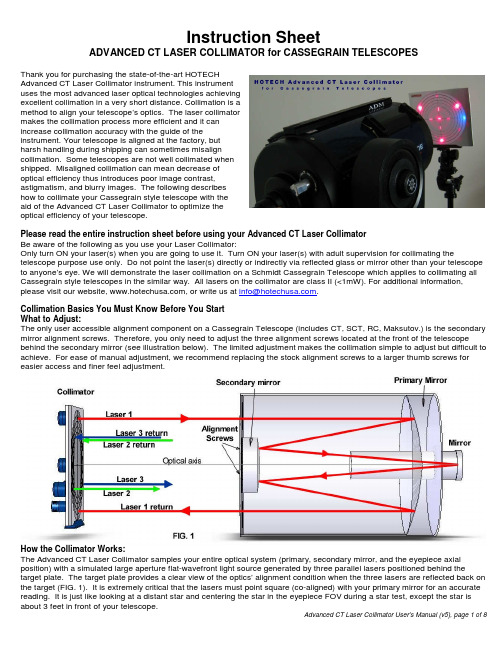
Instruction SheetADVANCED CT LASER COLLIMATOR for CASSEGRAIN TELESCOPESThank you for purchasing the state-of-the-art HOTECHAdvanced CT Laser Collimator instrument. This instrumentuses the most advanced laser optical technologies achievingexcellent collimation in a very short distance. Collimation is amethod to align your telescope’s optics. The laser collimatormakes the collimation process more efficient and it canincrease collimation accuracy with the guide of theinstrument. Your telescope is aligned at the factory, butharsh handling during shipping can sometimes misaligncollimation. Some telescopes are not well collimated whenshipped. Misaligned collimation can mean decrease ofoptical efficiency thus introduces poor image contrast,astigmatism, and blurry images. The following describeshow to collimate your Cassegrain style telescope with theaid of the Advanced CT Laser Collimator to optimize theoptical efficiency of your telescope.Please read the entire instruction sheet before using your Advanced CT Laser CollimatorBe aware of the following as you use your Laser Collimator:Only turn ON your laser(s) when you are going to use it. Turn ON your laser(s) with adult supervision for collimating the telescope purpose use only. Do not point the laser(s) directly or indirectly via reflected glass or mirror other than your telescope to anyone’s eye. We will demonstrate the laser collimation on a Schmidt Cassegrain Telescope which applies to collimating all Cassegrain style telescopes in the similar way. All lasers on the collimator are class II (<1mW). For additional information, please visit our website, , or write us at .Collimation Basics You Must Know Before You StartWhat to Adjust:The only user accessible alignment component on a Cassegrain Telescope (includes CT, SCT, RC, Maksutov.) is the secondary mirror alignment screws. Therefore, you only need to adjust the three alignment screws located at the front of the telescope behind the secondary mirror (see illustration below). The limited adjustment makes the collimation simple to adjust but difficult to achieve. For ease of manual adjustment, we recommend replacing the stock alignment screws to a larger thumb screws for easier access and finer feel adjustment.How the Collimator Works:The Advanced CT Laser Collimator samples your entire optical system (primary, secondary mirror, and the eyepiece axial position) with a simulated large aperture flat-wavefront light source generated by three parallel lasers positioned behind the target plate. The target plate provides a clear view of the optics’ alignment condition when the three lasers are reflected back on the target (FIG. 1). It is extremely critical that the lasers must point square (co-aligned) with your primary mirror for an accurate reading. It is just like looking at a distant star and centering the star in the eyepiece FOV during a star test, except the star is about 3 feet in front of your telescope.To ensure accurate aiming, you must use the crosshair laser emitting from the center of the collimator as a guide to the center point on your primary mirror (FIG. 2A), and the reflected crosshair from the telescopes primary mirror to the center point of the target (FIG. 2C). Please expect to spend most of the time on iterating the aiming adjustment. Be patient and consistent, the reward is beyond your imagination.How to Adjust Collimation on Your Scope:You can collimate your telescope at almost any position (e.g. telescope 20 deg. up) as long asboth the collimator and the telescope point square at each other. Once the lasers and yourtelescope are co-aligned, adjust the necessary secondary alignment screws gently to move thethree projecting laser dots to line up on the same track on the target plate.Process Flow Chart:1. Setup collimator distance2. Install reflector in eyepiece3. Aim collimator at telescope (FIG. 2A)4. Aim telescope at collimator (FIG. 2C)5. Adjust secondary to bring the three laser dots on the same trackPackage Content:1 x Premium Soft Carrying Case1 x Advanced CT Laser Collimator1 x SCA Reflector Mirror (1.25” or 2”)1 x 3V, CR123 Lithium Battery1 x Paper Ruler1 x External alignment Tab Strap(in bottom layer)3 x Alignment Tabs (in bottom layer)1 x Users Manual (in cover pocket)1.0. Setting Up the Laser Collimator on the Tripod1.1. Where to setup the telescope and the collimatorStation both the collimator and the telescope on a solid ground (no carpeted, wooden floor, or any other surface that will flex or vibrate). It is required to have both stationed on the same ground floor.1.2. Setup the collimator on the tripoda). Fasten the laser collimator on the recommended fine adjustment stage with the threadknob on the mount to the ¼-20 screw hole at bottom of the rail base.b). Further lock the thread knob with the fly wheel lock.c). Use the standard ¼-20 screw on your tripod to fasten the fine adjustment stage.2.0. Getting Familiar with Your Instrument2.1. Installing the batteryUnthread the battery compartment cap then insert the CR123 lithium battery with the positive side up(tip side up) then close the battery cap.2.2. Switching the laser to the proper modePosition the collimator on a tripod about 4 feet distance from a white wall with the target side facingthe wall. Rotate the rotary knob on the top right corner of the collimator to activate different lasermodes. You will see the projecting laser patterns on the wall activating at various positions.Mode 0: Unit off.Mode 1: Crosshair laser ON.Mode 2: Crosshair laser and three alignment lasers ON.Mode 3: Crosshair laser, three alignment lasers, and target backlight ON for night use.Other modes:DT: Three alignment lasers ON.BL: Backlight ON.1L: Crosshair laser and backlight ON.CL: Three alignment lasers and backlight ON.This is a logic switch. Other modes are for visual preferences that will not affect the collimation process. Please use the recommended mode in each procedure for best result.2.3. Gross pointing adjustmentSwitch the laser to Mode 2, lift the tripod and move the collimator with the tripod at variousdistances from the wall to see how the crosshair expands and reduces in size in reference todifferent distances.2.4. Fine adjustment stage adjustmentPlace the tripod with collimator back on the ground. Find and adjust the corresponding knob onthe stage in the following.Vertical Adjustment:- The large knob, on right, is for quick rough adjustment in the vertical direction. You can loosenthe large knob and level the laser first.- The forward small knob is for fine adjustment in the vertical (up/down) direction. You must lockthe large knob first in order to make the fine adjustment with the forward knob.Horizontal Adjustment:- The left side small knob is for fine adjustment in the horizontal (left/right) direction.3.0. Adapting the SCA Reflector Mirror:3.1. Adapting the SCA Reflector Mirror on your focuserIf the purpose of the night is visual observation, you may adapt the SCA Reflector with the diagonal,on the condition that it does not introduce optical aberrations (center of the field is not shifted if thediagonal rotates in the drawtube). However, if photography or CCD imaging is planned, it is best toadapt the SCA Reflector without the diagonal.For an installation video guide of the SCA mechanism, please review our YouTube videos at/hotechusa under Installing and Uninstalling HOTECH SCA Laser Collimator.4.0. Do You Need the External Alignment Tabs?- It is very critical to have the lasers co-aligned with your primary mirror optical axis for an accurate diagnosis of your telescope. To achieve this, you use the projecting crosshair on the collimator to center point your primary mirror byreferencing the 4 corners on the mirror to the crosshair lines. Then you use the reflected crosshair lines projected on the primary mirror to center point back to the target.- The crosshair lines from the collimator are precisely 90 degrees apart. You will have to find or create the 90 degrees markings on or close proximity to your primary mirror for collimator aiming reference.- It is ideal to edge-mark the 4 corners (90 degrees apart) on the primary mirror or the cell holder if it is accessible. For those scopes that do not have accessible open truss configuration, please refer to the following solutions.4.1. Visible components close to the primary cell – no Alignment Tabs neededMost Meade SCT telescopes have at least 4 visible mounting screws at the base of the telescope 90 degrees apart, protrude into the OTA. Identify the position of these 4 screws by looking from the front of your telescope. You will rely on these screwsas your collimator aiming guide. You will not need the external Alignment Tabs for your telescope if the mounting screws arevisible. Please proceed to step 5.0.4.2. No visible components close to the primary cell – require Alignment TabsIf there are no visible markings or objects in close proximity to the primary mirror that are 90 degreesapart, use the included Alignment Tabs as your alternative external aiming guide.4.3. Setting up the Alignment Tabs4.3.1. Measure and mark the 4-corner distance on your OTAa). Use the included paper strip ruler and wrap it onthe OTA closest to the primary mirror position.b). Mark the position where the paper strip interceptsto a full diameter wrap.c). Remove the paper strip. Line up the start of thestrip with the marked position and fold it twice tofind the ¼ length of your OTA diameter. d). Wrap the paper strip back on your OTA, and use amarker or pencil to mark three consecutivepositions 90 degrees apart on your OTA.ab c d 4.3.2. Installing the Alignment Tabsa). Wrap and tighten the black strap around the OTA next to the 3indexed markers on the OTA.b). Insert the base of three Alignment Tabs at the correspondingpre-marked position.c). Pre-adjust the Alignment Tabs to make it tangent to the OTA.A b c4.3.3. Lining up the Alignment Tabs normal to the OTAIt is important to keep the Alignment Tabs tangent to the OTA at eachmarked position for an accurate aiming reference. Use the crosshairlaser on the collimator to help you achieve this step.a). Position the laser collimator at about the same center height of yourtelescope. Switch to Mode 1 to activate the crosshair laser.b). Aim the crosshair directly at the visual back of your telescope toproject the crosshair on the 4-edge marks. Check the reflection ofthe crosshair laser on the target from the SCA reflector and adjustboth pointing of the collimator and the telescope to bring thereflected crosshair back to the center of the target on the collimator.c). Iterate the process until both the projecting crosshair on yourtelescope is on the 4-edge marks and the reflected crosshair is inthe center of the target.d). Adjust the Alignment Tabs to line up with the crosshair to the end ofthe Alignment Tab. This will ensure the tabs are pointingnormal/tangent to the OTA. You will rely on these tabs duringcollimation. Switch to Mode 0 to turn off the laser collimator.a &b b &c b & cd d5.0. Positioning the Laser Collimator at the Proper DistanceThe distance between the laser collimator and yourtelescope varies depending on the diameter and focaldistance of your telescope. In general, the longer thedistance away from your telescope, the higher accuracy youwill achieve. And in practice, any distance beyond the focaldistance will be sufficient for your calibration for both visualand practical adjustment purposes. In this procedure, wewill help you identify the best collimating distance for yourtelescope.5.1. Determine the distance between the laser collimator and your telescopea). Position the collimator in front of the scope to about equal length of the OTAwith the target display facing the telescope (photo above).b). Switch the collimator to Mode 1 (crosshair laser only).c). Roughly aim the crosshair toward the telescope.d). Experiment with the proper distance by slightly lifting the tripod, with thecollimator on it, and move the collimator slowly toward and away from thetelescope while keeping the reflected crosshair on the target plate. Don’t worryabout getting the crosshair perfectly concentric in the center of the target at thispoint. You will see how the crosshair contract and expands in size on the targetplate in relation to the distance adjustments.e). Move the collimator to where the crosshair converges to the smallest size. Thisis the back focal point of the primary mirror. Now begin to move the targettowards the telescope until the crosshair expands to the size of the first ring? onthe target.f). Firmly position the tripod at this distance. This will be your collimating distance.6.0. Achieving Co-Alignment on the Collimator and Your TelescopeThis is the critical stage where you must co-align the collimator and your telescope for an accurate reading of your optics alignment. DO NOT use the center of the secondary mirror assembly as your crosshair centering reference because the secondary mirror might not be center positioned on the corrector plate, and the telescope might not be pointing straight at the collimator at this point. You can use it as a quick gross adjustment, but not for final aiming adjustment.6.1.1. For telescopes using the internal screws as the aiming referencea). Check if the crosshair is visible on the internal screws.b). Aim the crosshair emitting from the collimator on your telescope’s 4-corner referencingedges (the internal screws). Us the fine adjustment stage to refine the collimator aiming.c). Go to step 6.2 (next page).6.1.2. For telescopes using the Alignment Tabs as the aiming referencea). Check if the crosshair is visible on the three tabs.b). Point the crosshair as close to the center of the primary mirror, and wave your hand behindthe Alignment Tabs to find the crosshair. If the crosshair is cropped beyond the tip of thestick, move your collimator further away from the telescope until you can see a portion of thecrosshair projecting on the tip of the Alignment Tabs.c). Us the fine adjustment knob to refine the collimator aiming to line up with the threeAlignment Tabs.6.2. Aim your telescope back to the collimatora). Use the telescope’s fine adjustment knob or the motor remote control to aim the reflectedcrosshair from your telescope back to the center of the target. You will need to line up thevertical and horizontal cropped crosshair lines with the cross line on the target plate. When itpoints square, the vertical and horizontal cropped crosshair lines will have symmetry length.6.3. Co-alignment confirmationIterate step 6.0 until both conditions are met. This means both telescope and the collimator are pointing square at each other like looking at a distant star. Lock your telescope and you are ready to diagnose your optics.7.0. How to Read the Diagnostic Result on the CollimatorWith proper aiming in step 6, the collimator can accurately reveal any errors in your optical system by reading the center deviation of the three returning laser dots on the target plate.7.1. Locate the three laser dotsa). Switch to Mode 2 or Mode 3 (three lasers and the crosshair, or Mode 3 with backlight).b). Verify if the crosshair is still center pointed on both the target plate and the Alignment Tabs or screw markers?.c). Locate the three laser dots on the target plate.d). If the three laser dots are visible on the target plate, go to step 8 to collimate your telescope.e). If the three laser dots are not visible or partially visible on the target plate, please continue to the following possiblescenarios.7.2. The SCA Reflector is not properly adapteda). The SCA Reflector represents the axial alignment of your drawtube (eyepiece holder). You must install it correctly (squarein your drawtube) in order to represent the axial position of your eyepiece or CCD camera position. This axial position of your drawtube is directly related to the alignment axis of your entire optical system (telescope). Please refer to step 3 for proper SCA Reflector installation guide.b). If you have verified the correct installation, and still exhibit the same condition, continue to the next step, otherwise go tostep 8.7.3. The SCA Reflector is not positioned at the focal planea). This can happen if you were initially using the diagonal for viewing, thus the focal plane is at the diagonal extensiondistance. After you remove the diagonal for collimation, without any focusing adjustment, it will move the three laser dots out of the target screen. If you do not use the diagonal, continue to the 7.4.b). Adjust the focus to bring at least two laser dots into the full view of the target plate. Adjust the focus in one direction first tosee if any of the laser dots are moving toward the center direction of the target. If the laser(s) is moving or expanding away from the center of the target, reverse the focusing direction to bring at least two laser dots into the full view of the target plate. Go to step 8 to collimate your telescope.7.4. Your telescope is grossly out of alignmentWhen your telescope is grossly out of alignment, the laser dots may be completely out of the target screen. You may start the collimation process to see if you can bring the three laser dots into the target screen. Proceed to step 8.0.8.0. Collimating Your TelescopeThe main objective in this step is to bring the three laser dots on the same track on the target. You will need to constantly check the crosshair laser (step 6) for both telescope and collimator aiming on each iterated adjustment. Here are few simple precautions you need to follow while adjusting the secondary mirror alignment screws located on the back of the secondary mirror assembly or front center of the telescope.a. Never touch the central screw which holds the secondary mirror.b. The three screws must be turned in moderation, no screw being over-tightened or totally unscrewed.c. When a screw is turned, the other two must be tightened. Never keep more than one screw loose.d. Each turn on the screws must be small. Reference the screw adjustment to the displacement of the three laser dots on the target plate to determine your adjustment level.8.1. Collimate your telescopea). Adjust the alignment screws to bring the three reflected laser dots on the same track on the target.b). If you cannot bring all three laser dots into the target view because the dots are too far apart, adjust the focus to merge thethree laser dots at approximate distance between track 4 & 5. c). Check for proper aiming of the collimator and the telescope in step 6.The telescope might shift in position if you put too much pressure during secondary mirror adjustment. You must doublecheck if you have nudged the telescope pointing out of the co-alignment.d). Iterate step 8.1 until both the three laser dots are on the same track on the target and the aiming of both the collimator andtelescope are still co-aligned.9.0. Verifying and Fine Tuning Your Collimation9.1. Star test to verify the adjustmenta). On your first observing session, star test the telescope to verify the adjustments.The Advanced CT Laser Collimator should bring excellent collimation to your telescope. Minor adjustment might berequired due to temperature variation during a long observing session.b). Use the intra-focal and extra-focal technique with a high magnification eyepiece on a magnitude 0 to 1 star to determinethe result. Fine tune the collimation if necessary. Please refer to the Star Collimation manual for detail. You are ready for observing after final touch up. 10.0. Possible Scenarios if the Laser Collimation Does Not Agree with Star Collimation10.1. Both the collimator and the telescope were not co-aligned during adjustmentIt is possible that during collimation (step 8), the co-alignment of the collimator and the telescope were slightly off causing an incorrect diagnosis. It is very critical to ensure both the collimator and the telescope are co-aligned to simulate the light path entering the telescope.Do not adjust the collimation screws. Go to step 6 to verify the co-alignment of the collimator and the telescope and check if three laser dots still fall on the same track. If both conditions are met, your optical system is in good condition meaning they’re all lined up well on the same optical axis. If not, continue to the next step.10.2. The mirror-flop on your primary mirror focusing mechanism is causing the miscollimationDue to machining tolerances on the primary mirror and improper greasing on the baffle, some telescopes exhibit more mirror-flop then others. A slight loose tolerance will cause major axial alignment deviation. The Advanced CT Laser Collimator is sensitive enough to pick up any deviation in step 6. Prior adjusting the secondary alignment screw, observe the shiftingposition of the three laser dots on the target by making two full turns clockwise on the focus knob, then reverse half turn. The shifting of the laser dots during the reverse turn tells how much mirror flop you have on your focusing mechanism.If the displacement is more than 2 tracks spacing distance, we recommend attaching a higher grade focuser on your visual back for focusing adjustment and leave the built-in focus mechanism untouched.10.3. The eyepiece drawtube or the visual back is not square to your primary mirrorWe recommend replacing a new higher grade eyepiece drawtube or a focuser that has tip/tilt adjustment to correct the axial error. E.g. MoonLite CS model, /cgi-bin/dman.cgi?page=productdetail&plugin=dstore.cgi&product=CS . We have found several older SCT scopes having poorly machined eyepiece/drawtube which is not square to the OTA. This may cause serious problem for imagers where the focal plane are also not parallel to the primary.。
EarthVision操作手册

还有一个比较重要的文件是井数据文件, 还有一个比较重要的文件是井数据文件, 用它来产生井标注文件, 用它来产生井标注文件,也用它来对构 造图进行校正,文件格式形如上图所示, 造图进行校正,文件格式形如上图所示, 第一列是井名,第二列是X坐标,第三列 第一列是井名,第二列是 坐标, 坐标 坐标, 是Y坐标,第四列是补芯海拔,第五列是 坐标 第四列是补芯海拔, 目的层钻井深度,第六列还可以增加其 目的层钻井深度, 他分层井深,或是底深。 他分层井深,或是底深。
T0和断层数据格式: 和断层数据格式: 和断层数据格式
T0数据格式 数据格式
断层数据格式
上图为T0数据格式,第一 二 上图为 数据格式,第一,二,三列分别 数据格式 坐标和T0值 为x,y坐标和 值。 , 坐标和
上图为断层数据格式,第一 二 上图为断层数据格式,第一,二,三列分 别为x, 坐标和断层号 坐标和断层号。 别为 ,y坐标和断层号。
依此, 依此,把其它所有的离散数据文件都加 上文件头。 上文件头。 注意:断层文件的断层号名称用Lineid ; 注意:断层文件的断层号名称用 测网文件的测线名也用Lineid 井数据文 测网文件的测线名也用 件的井名用Wellid ,补芯海拔、钻井深度 补芯海拔、 件的井名用 补芯海拔 等的名称用户自己能识别开就可以了。 等的名称用户自己能识别开就可以了。
EarthVision的主界面及各菜单的主要功能: 的主界面及各菜单的主要功能: 的主界面及各菜单的主要功能
显示列表文件 改变目录 推出DGI 推出
其中List files选项可以选择文件并对 其中 选项可以选择文件并对 文件进行一些简单的编辑和操作。 文件进行一些简单的编辑和操作。 Change directory选项主要是设置文 directory选项主要是设置文 件存放的目录, 件存放的目录,和Zmap里面设置路径 里面设置路径 等同。 等同。
Geoscope地质放大镜参考文档

属性融合
③ 属性融合—双色标组合(形+值)
小角度
大角度
多角度融合
属性融合
④ 属性融合—三色标组合显示
颜色代表地层方位角(0-360) 亮度代表地层倾角(0-7)
0 7
90
0
270
180
相干
⑤ 属性融合—透明叠合显示
属性融合
12 21
3 3
4 4
主水道 废弃水道 废弃水道
56
5 6
倾角 相干
提纲
(反演子系统)
模型反演 反射系数反演 分频属性反演 贝叶斯稀疏脉冲反演
Geoseis
(地震子系统)
品质增强 时频属性 几何属性 烃类检测
提纲
一、概论 二、底层功能 三、Geolog地震岩相子系统 四、Geoseis地震属性子系统 五、Geostrat地震沉积子系统 六、Geoinversion地震反演子系统
属性融合
• 根据色素理论,将多个(2或 3)切片融合显示。
• 显示方式有:双色标透明度 叠合、二维色标融合、三色 标(RGB、HSV)融合等。
• 用于突出沉积特征或储层的 成像,为沉积解释和储层追 踪服务。
① 属性融合—RGB融合
RGB融合平面图
属性融合
单频平面图
属性融合
② 属性融合—单色标组合(形+值)
地震数据播放
地震资料显示
142030H0HzHzz
观察不同单频体在地震上的差异,实现快速浏览。
层位、断层解释
可进行层位和断层的剖面解释和断层多 边形的平面组合。
2
16
切片显示与播放
年代地层切片--虚切片
• 虚切片是本软件地震沉积学 分析的基础。
SCIENTIFIC PHYSICS 3B 谱测器操作手册说明书
3B SCIENTIFIC ® PHYSICS1Steuereinheit für Kritisches-Potenzial-Röhren (115 V, 50/60 Hz) Steuereinheit für Kritisches-Potenzial-Röhren (230 V , 50/60 Hz)1000633 (115 V, 50/60 Hz) 1008506 (230 V, 50/60 Hz)Bedienungsanleitung01/14 ALF1 Ausgang Beschleuni-gungspannung2 Eingang Picoampere-verstärker3 Anschlussfeld Multimeter4 Anschlussfeld Oszilloskop bzw. Data-Logger5 Bedienfeld Ausgangs-spannung1. SicherheitshinweiseDie Steuereinheit für Kritisches-Potenzial-Röhren entspricht den Sicherheitsbestimmun-gen für elektrische Mess-, Steuer-, Regel- und Laborgeräte nach DIN EN 61010 Teil 1. Sie ist für den Betrieb in trockenen Räumen vorgese-hen, die für elektrische Betriebsmittel geeignet sind.Bei bestimmungsgemäßem Gebrauch ist der sichere Betrieb des Gerätes gewährleistet. Die Sicherheit ist jedoch nicht garantiert, wenn das Gerät unsachgemäß bedient oder unachtsam behandelt wird.Wenn anzunehmen ist, dass ein gefahrloser Betrieb nicht mehr möglich ist (z.B. bei sichtba-ren Schäden), ist das Gerät unverzüglich außer Betrieb zu setzen.2. BeschreibungDie Steuereinheit dient zum Betrieb der Kriti-sches-Potenzial-Röhren S mit He-Füllung (1000620) und mit Ne-Füllung (1000621).Das Gerät stellt eine sägezahnförmige Span-nung mit einer Frequenz von 20 Hz als Be-schleunigungsspannung für die Anode bereit. Diese Spannung ist von der Betriebsmasse des Geräts galvanisch getrennt. Dadurch kann eine zusätzliche, vom Benutzer wählbare Spannung wie z.B. eine Batterie zwischen Anode und Auf-fängerelektode angelegt werden. Die Start- und Endspannung des Sägezahngenerators lassen sich stufenlos zwischen 0 und 60 V einstellen. Hierdurch ist eine exaktere Betrachtung eines bestimmten Kurvenabschnitts möglich.Mit Hilfe des eingebauten Picoampereverstär-2kers kann der Kurvenverlauf des Auffänger- stroms auf einem Oszilloskop dargestellt wer-den. Durch die eingebaute SLOW-Funktion mit geringerer Frequenz(ca. 1/6 Hz) kann diese Kennlinie auch mit einem langsameren Messin-terface oder einem XY-Schreiber aufgenommen werden.Das Gerät mit der Artikelnummer 1000633 enthält ein Stecker-Netzgerät für eine Netzspannung von 115 V (±10 %), 1008506 eins für 230 V (±10 %).2. BedienelementeAusgang 1 dient zur Bereitstellung der Säge-zahn-Beschleunigungsspannung U A . Die Start-spannung wird über Regler 4, die Endspannung über Regler 3 eingestellt.Zum Einstellen der gewünschten Parameter der Sägezahnspannung kann ein Multimeter ange-schlossen werden. Zwischen Buchse 3 und Masse (UA MAX) bzw. Buchse 4 und Masse (U A MIN) wird eine um den Faktor 1000 kleinere Spannung gemessen.Der Auffängerstrom I C(pA) wird über Eingang 2 (BNC-Buchse) dem Gerät zugeführt. Verstärkt durch den internen Picoampereverstärker kann der Strom über das Anschlussfeld Oszil-loskop/Data-Logger als äquivalente Spannung (1 V/nA) abgenommen werden.Zur Darstellung des Auffängerstroms in Abhän-gigkeit der Beschleunigungsspannung kann der XY-Modus eines Oszilloskops verwendet wer-den. Hierzu können am Ausgang FAST die je-weiligen Spannungen mit 20 Hz abgenommen werden.Über den Ausgang SLOW können die Werte mit geringerer Frequenz an ein Interface oder einen XY-Schreiber ausgegeben werden. Die Ausga-be wird über ein integriertes Abtastverfahren mit der Taste SLOW RUN gestartet.Bei eingeschalteter SLOW-Funktion leuchtet die LED grün, ist die Funktion beendet leuchtet sie wieder rot.In beiden Fällen dient jeweils für die Ausgabe der Sägezahnspannung Buchse 1 (Y - Ablen-kung) und für die Ausgangspannung des Mess-verstärkers Buchse 2 (X - Ablenkung).3. Technische DatenVersorgungsspannung: 12 V AC Strommessung: 1 V / nA, BNCAusgangspannung: 0 - 60 V / 20 Hz, säge-zahnförmigMessausgabe: Buchse 1: 0 - 1 V, propor-tional zur Ausgangsspan-nung Buchse 2: 0 - 1 V, propor-tional zum Auffän-gerstrom I C Betriebsarten: FAST: Messausgabe 20 Hz SLOW: Messausgabe 1/6 Hz Abmessungen: ca. 170x105x45 mm 33B Scientific GmbH ▪ Rudorffweg 8 ▪ 21031 Hamburg ▪ Deutschland ▪ Technische Änderungen vorbehalten © Copyright 2014 3B Scientific GmbH4. Bedienung•Steuereinheit mit dem Steckernetzgerät verbinden. Die Anschlussbuchse dazu be-findet sich auf der Unterseite des Geräts. • Steuereinheit in den Schaltkreis der Kriti-sches-Potenzial-Röhre einbauen.•Zum Aufbau und zur Durchführung des Ex-periments Bedienungsanleitung der Kriti-sches-Potenzial-Röhre lesen.•Steckernetzgerät ans Netz anschließen. Die LED leuchtet rot.5. Entsorgung•Sofern das Gerät ver-schrottet werden soll, so gehört dieses nicht in den normalen Haus-müll. Es sind die lokalen Vorschriften zur Entsor-gung von Elektroschrott einzuhalten.Fig. 1 Beschaltung der Kritisches-Potenzial-Röhre。
斯派克直读光谱仪操作手册
斯派克直读光谱仪操作手册SPECTRO光谱仪的分析软件结构主要由三部分组成Analysis 分析模式Method 分析方法Config 系统文件在这一章中,我们首先向大家介绍Analysis分析模式,日常工作中,我们大部分的工作都是在Analysis分析模式下来完成。
一、光谱操作的准备工作光谱仪的分析软件采用的是标准的WINDOS操作环境,所以要求操作员有一定的计算机知识,如果您在操作光谱仪前对微软公司的WINDOS不熟悉的话,请先熟悉WINDOS操作的基本知识。
二、键盘与鼠标的使用众所周知WINDOS操作系统的最大优点就是操作灵活,可同时打开多个窗口。
为了方便于鼠标与键盘的同时操作,我们分析软件中的只要功能也设计成既可以使用键盘,也可以使用鼠标来进行操作,在下面的章节中,我们会详细的介绍给用户。
三、键盘上功能键的介绍四、Analysis View模式下菜单的介绍FileNew…………………………………………………………建立新的程序Open…………………………………………………………打开已储存的分析数据库Save…………………………………………………………储存数据Save As……………………………………………………另存为Print…………………………………………………………打印分析数据Exit…………………………………………………………退出分析程序AnalysisLoad Method………………………………………………调分析程序Single Measurement………………………………………开始测量SampleIdent………………………………………………标题头内容Globle standardization……………………………………通用标准化Standardization……………………………………………标准化Standardization results……………………………………标准化结果Apply Type standardization………………………………应用类型标准化Type standardization Sample……………………………类性标准化样品Calibratio n Sample………………………………………做工作曲线样品Delete single………………………………………………删除单次测量结果Delete Results……………………………………………删除分析结果Delete All…………………………………………………删除所有分析结果Show/Hide Sample Info…………………………………未开发窗口ViewNaviogate…………………………………………………窗口转换Analysis……………………………………………………分析窗口Method……………………………………………………方法窗口Config……………………………………………………参数窗口Docking Views……………………………………………工具栏选择Navioate bar…………………在屏幕左侧显示Analysis,Method,Config三个窗口Display Bar……………………显示平均结果及他们的标准偏差和相对标准偏差Smaple ID………………………………………………显示样品编号Toolbar…………………………………………………显示工具吧Status Bar………………………………………………状态吧Initialize…………………………………………………仪器初始化Reprofile Optic…………………………………………扫描Perform Constant Light Test……………………………恒光测试Switch Analytical Flow On/Off…………………………冲洗氩气控制开关Start Cleaning Flush……………………………………清洁时执行氩气冲洗Reset SPARK…………………………………………激发次数回零Setup Devices…………………………………………设备的建立Global Database………………………………………通用数据库Content………………………………………………帮助内容Help Index……………………………………………软件说明Spectro Homepage……………………………………斯派克网页About Spark Analyzer…………………………………分析软件的版本五、如何完成标准化(Standardization)无论是何种类型的光谱分析仪,日常的标准化工作都是非常重要的的操作环节,因为标准化的正确与否是直接影响分析结果精确的关键,也是我们在日常分析中要经常执行的功能之一。
GO-SPEX500空间光谱辐射计快速操作指南S1
GO-SPEX500空间光谱辐射计快速操作指南1 准备工作1.1为保证测试精度,环境温度推荐控制在25±1℃。
1.2光源在测试前要进行老炼,若已经经过老炼无需此进行步骤。
1.3测试前要准备必要的夹具。
1.4准备内六角扳手、螺丝刀、万用表等常用工具以及导线若干。
2 灯具配光测试主要测试灯具的电参数、配光和灯具效率等参数。
2.1 装夹灯具在装夹时要注意灯具的中心与转台的转动中心要重合,可以利用十字激光对准器进行对准。
安装时建议对于C0平面位置要用记号笔作标志。
2.2 灯具照片灯具夹装在分布光度计上后,可再拍几张照片。
这些照片的某一张可以用于测试报告中以增强报告的可读性,同时也便于出现问题后分析问题。
2.3 测试正确接线。
点亮灯具。
用功率计记录灯具的电参数。
根据灯具发光口面的大小,调整可移动光阑片开孔的大小,保证探测器能“看到”整个灯具发光面,调整完毕后可关闭暗箱门。
监视并等待灯具发光稳定,一般都要30分钟以上或更长。
软件操作:点击“操作”菜单下的“配光测试”进入测试,在测试信息对话框中输入相关的信息,确认输入正确的测试距离(仅在第一次使用软件时需要输入)。
在测试光源处选择“室内灯具”或“道路灯具”等,在光源数据处输入光源额定光通量和实测光通量。
若是LED灯具,可选择“为整体式灯具类型”选项。
输入完后,按确定进入测试界面进行测试。
测试界面如图1所示。
测试角度一般按用户手册5.3节设置。
.图1 配光测试界面2.4 注意事项◆电参数请务必记录。
◆测试距离务必设置正确。
3 文件保存3.1 测试完成后,软件会自动提示用户保存文件,用户设置好保存路径和文件名即可。
文件保存格式为*.GOS,此格式只能用远方GOSoft软件打开。
3.2 规范测试信息在GOSoft软件中要输入厂商、灯具名称、型号等信息,这些信息可以在测试完成后再在软件中修改。
但存档之前建议把这些信息输入齐全,以便于以后查看报告。
3.3 打印报告参照GO-SPEX500用户手册5.3节。
GeoMapper4.0 用户手册
GeoMapper 4.0 Android 用户手册
北京合众思壮科技股份有限公司
目录
第一部分 软件安装................................................................................................................................ 7 一. 系统运行环境................................................................................................................................ 7 1.1 硬件环境................................................................................................................................... 7 1.2 软件环境................................................................................................................................... 7 二. GeoMapper Office 软件安装......................................................................................................... 7 第二部分 G
- 1、下载文档前请自行甄别文档内容的完整性,平台不提供额外的编辑、内容补充、找答案等附加服务。
- 2、"仅部分预览"的文档,不可在线预览部分如存在完整性等问题,可反馈申请退款(可完整预览的文档不适用该条件!)。
- 3、如文档侵犯您的权益,请联系客服反馈,我们会尽快为您处理(人工客服工作时间:9:00-18:30)。
Geoscope地质放大镜用户手册诺克斯达石油科技Geoscope地质放大镜用户手册诺克斯达石油科技目录第一章概述 (1)1.1软件概况 (1)1.2软件技术思路 (1)1.3软件系统构成 (1)1.4软件总体逻辑架构 (1)1.5软件平台 (2)第二章数据加载 (3)2.1地震资料加载 (3)2.2井资料的加载 (5)2.2.1时深关系的加载 (6)2.2.2井位加载 (7)2.2.3井轨迹加载 (9)2.2.4井曲线加载 (10)2.2.5井分层加载 (11)2.3层位数据加载 (12)第三章应用模块 (16)3.1GEOLOG部分 (16)3.1.1合成地震记录—— Synthetic (16)3.1.2岩石物理学分析—— Cross Plot (24)3.1.3特征曲线计算—— Log Tool (28)3.2GEOSEIS部分 (33)3.2.1道比例化——Trace Scaling (33)3.2.2分频去噪——Denoise (35)3.2.3提高分辨率处理——Decon (36)3.2.4瞬时属性—— Instant Attribute (41)3.2.5分频成像—— RSI (43)3.2.6倾角方位角——Dip Azimuth (44)3.2.7 分频属性相干—— Coherency (46)3.2.8有色反演—— SCI (48)3.2.9分频属性反演—— AVF Inversion (53)3.2.10吸收分析——Absorb Analysis Window (63)3.2.11 地震数据体处理器—— Cube Processor (65)3.3GEOSTRAT部分 (66)3.3.1 时窗属性——Time Window Attr (66)3.3.2 波形结构分析——Seismic MacroFace (70)3.3.3 频谱成像—— Spectrum Imaging (73)3.3.4 时频三原色——RGB (76)第四章界面介绍 (79)4.1主窗口介绍 (79)4.2剖面显示 (80)4.3切片显示 (83)4.4任意线的显示 (89)4.5井数据的显示 (90)4.5.1井数据的时深转换 (91)4.5.2井位及井轨迹的显示 (91)4.5.3井曲线的显示 (93)4.5.4井分层的显示 (94)4.6层位显示与解释 (94)第一章概述1.1软件概况Rockstar公司是一家地球物理软件开发公司和项目服务公司。
其产品GeoScope具有独立自主产权,是专门针对隐蔽油气藏勘探而开发的一套技术体系和软件支撑平台,在全国已有十多个用户,其推动的技术体系和应用理念已在多个大型项目上成功应用。
1.2软件技术思路隐蔽油气藏由于没有外部构造形态,含油气圈闭难以确定。
对于隐蔽油气藏勘探和开发,首先要搞清隐蔽油气藏的成藏模式,在关键界面附近找地层圈闭油气藏,在层序单元部寻找岩性油气藏,为此需要建立井震统一的年代地层格架需要进行体系域控制下的沉积体系分析,需要相控下的储层预测。
Geoscope 就是为了实现上述分析而开发的一个软件平台。
1.3软件系统构成GeoScope是专门为隐蔽油气藏研究而开发的软件包,包括:Geostrat,Geoseis,Geolog 三个子系统。
Geostrat提供了一个多体的构造层序解释环境,提供了三种地震微相的分析方法,提供了一种三相综合分析的工具。
Geoseis提供了为岩性预测而服务的多种专项技术,这些技术包括道比例化、提高分辨率、反演、属性提取等。
Geolog提供了反演和测井层序地层分析的各种辅助功能。
1.4软件总体逻辑架构以下是Geoscope常用模块的逻辑关系图,它既是一种应用平台也是一种工作流程,它体现了以地震资料为核心,地质资料和测井资料相配合的相控储层预测技术体系。
其中物探、地质和测井的结合技术是其关注的重点,三相分析和相控预测是其核心理念,井震格架下的构造研究、岩相分析、储层研究是其追求的目标。
Geoscope 应用框架平台1.5软件平台Geoscope是在QT环境下用C++开发的,所以它可以安装在微机的Windows2000及以上和Linux Red Hat9.0环境下,也可以安装在SUN、Solaris2.8及以上工作站上。
Geoscope可以开放其底层接口,以便于用户在其上开发应用模块插件,是软件自主创新的理想平台。
第二章 数据加载启动主界面安装完成后会在主界面上出现Geoscope 的图标,双击此图标就会弹出如下主界面:Geoscope 主界面2.1地震资料加载在主界面中点击Project ->New 即出现如下界面,给要创建的项目选择路径和项目名称,在Add File 中选择segy 数据体。
选好参数后左键点击Scan 按钮后点击Next 按钮。
设置项目目录 设置项目名称加载地震数据体 线道号位置X 、Y 坐标位置数据体名称扫描数据体点击Create后得到如下界面如上图,将数据体Cube1左键直接拖入中间空白区域即可在右方出现工区底图。
向已产生的项目中加载数据体时,在项目数据列表中的“Seismic Cube”节点的右键菜单中选择“Import”项,会弹出数据体加载窗,与创建项目时加载地震数据体相似。
2.2井资料的加载以下所有类型的井数据加载文件都必须是以空格分隔的ASCII码文件。
2.2.1时深关系的加载在Well的ChkSht处右键点击ChkSht->Import得到如下图界面加载时深关系。
CheckShot File ——时深关系文件,点击右侧按钮选择文件。
TVD ——垂深;Time ——时间;Unit ——单位;Colume ——属性数据所在列号;设置好以上参数后点击Load自动加载。
加载成功后在项目列表的“ChkSht”节点下出现该时深关系的图标。
2.2.2井位加载在Well->Well右键点击Well—>Import Well得到下图所示界面加载井位。
Well File ——井位文件,点击右侧按钮选择井位文件;Name ——井名;X —— X坐标;Y —— Y坐标;Max MD ——最大测深(可不选);Unit ——单位;Column ——所在列号;X Shift ——井位文件中X坐标的漂移量;Y Shift ——井位文件中Y坐标的漂移量;以上两项用于井位文件中的X、Y坐标与地震数据体中的坐标不匹配时,通过设置漂移量来正确加载井位数据。
设置好以上参数后点击Load自动加载井位。
井位数据加载完成后,在项目列表中的“Well”节点下,会出现加载成功的井。
2.2.3井轨迹加载如上图所示,右键点击井图标,选择Import Deviation菜单项后,弹出如下图所示窗口加载井轨迹数据:有关参数:MD ——测深;TVD ——垂深;AZI ——方位角;INCL ——倾角;X ——绝对X坐标;Y ——绝对Y坐标;DX ——相对前一点的X位移量;DY ——相对前一点的Y位移量;Unit ——单位;Column ——所在列号;有以下的几种加载方式:1、MD、AZI、INCL;2、MD、TVD、X、Y;3、MD、TVD、DX、DY;在完成以上参数设置后,点击Load完成加载。
井轨迹数据不显示在项目数据列表中。
2.2.4井曲线加载右键点击井图标,选择Import Log项,加载井曲线,窗口如下图通过“Browse”按钮选择曲线文件;在选定的列上,设置曲线类型、曲线名称、单位。
在设置完成曲线参数后,点击“Load”按钮完成曲线加载。
加载完井曲线后如下图所示:2.2.5井分层加载在项目数据列表中的“Well”节点处点击鼠标右键,选择“Import Tops”项,可以加载多井的分层;在某口井的图标处点击鼠标右键,选择“Import Tops”项,只能加载该井的分层数据。
加载分层如下图所示。
选择分层文件后点击Preview在窗口右侧给每个分层指定颜色。
参数:Well ――井名;Tops ――分层名;MD ――测深;Column ――属性所在的列数。
在设置完成相关参数后,点击“Load”按钮完成分层数据的加载,并且在项目数据列表中显示出来。
2.3层位数据加载层数据的加载文件必须是以空格分隔的ASCII码文件。
如上图所示,右键点击Horizon->New horizon得到如下窗口,给出要加层位名如g4_10,在Horizon目录下会出现该层位名。
右键点击该层位名如上图所示:Import ——加载层位如下图,选择准备好得层文件。
要加载的层文件的格式应当如下图所示:Export ——输出层位;Color ——选择层位颜色;Remove ——删除该层位。
将该层位拖入中间区域时会弹出如下图左所示窗口来选择显示颜色,点击New弹出如下图右所示窗口给出颜色名称:左键双击上图左的颜色条弹出如下图所示窗口:Defined Color ——颜色方案;ColorBar Options:Inverse ——色标反转;Max /Min Value ——最大/最小值;Background Color ——背景色;第三章应用模块3.1 GEOLOG部分3.1.1合成地震记录—— SyntheticApplication->GEOLOG->Synthetic得到如下图所示界面(一)制作并保存合成记录方法一:Synthetic->Quick Create得到如下图所示窗口,选择数据体和井曲线后点击OK,其中DT Log是必须的得到如下图所示的窗口:方法二:也可以点击Synthetic->Well、Seismic、Checkshot、Wavelet 分别设置井数据、地震数据、时深关系和子波。
设置井数据:设置地震数据:设置时深关系:设置子波:做完合成记录后点击TIME按纽输出到时间域,如下图,给出合成记录以及每口井的CheckShot名称。
指定的时深关系指定的子波(二)调整合成记录调整方式有两种:Move(平移)和Strech(拉伸压缩)。
Break:停止编辑,转入显示状态。
Undo:撤消当前的编辑结果(只能撤消一次)。
1.Move(平移)在合成记录或剖面显示窗中,按住鼠标左键拖拽,会出现一条红线,将红线拖拽到指定位置,松开鼠标键后,程序自动完成合成记录的移动。
2.Strech(拉伸压缩)点击Strech项后,进入该模式,在合成记录窗与地震剖面窗中用鼠标左键分别设置相应的时间线(兰色虚线),用鼠标右键可以消除某条时间线,两组时间线由上至下一一对应,在设置完拉伸压缩时间线后,再次点击Strech项,程序将自动完成其工作。
3.显示参数调整Refresh:刷新显示。
(1) Well Parameter――设置井数据显示参数:在该窗口中,可以设置纵向显示比例、显示的起始结束时间、显示的曲线及显示的分层。