第七讲空间计量经济学模型的matlab估计
经济预测与决策技术及MATLAB实现第7章 时间序列预测法

预测图
7.2 指数平滑预测法
7.2.1 一次指数平滑法
(1)一次指数平滑法的基本模型
S (1) t
Xt
(1
)
S (1) t 1
S (1) t
Xt
(1 ) X t1
L
(1
)t
1
X1
(1
)t
S (1) 0
Xˆ t1
S (1) t
其中,X0, X1,L , X n 为时间序列观测值,
首页
7.2.2 二次指数平滑法
(1)二次指数平滑法的线性模型为
XˆtT at btT
at
2
S (1) t
S (2) t
bt
1
(St(1)
St(2) )
S (1) t
Xt
(1 )St(11)
S (2) t
S (1) t
(1 )St(21)
【例7-4】 (续例7-1) 用二次指数平滑法预测2016年投 资额(=0.9)。
当时间序列既有季节性变动又有趋势性变动时,先建 立趋势预测模型,在此基础上求得季节指数,再建立 预测模型。其过程如下:
(1)计算历年同季平均数r;
(2)建立趋势预测模型,求趋势值
(3)计算出趋势值后,再计算出历年同季的平均数R; (4)计算趋势季节指数(k);用同季平均数与趋势值同 季平均数之比来计算。 (5)对趋势季节指数进行修正;
88773.6 109998.2 137323.9 172828.4...
224598.8 251683.77 311485.13 374694.74
空间计量模型的估计方法

空间计量模型的估计方法我折腾了好久空间计量模型的估计方法,总算找到点门道。
说实话,这事儿我一开始也是瞎摸索。
我最开始接触的时候,真是一头雾水。
我就先从那些基础的计量方法看起,什么最小二乘法啊,感觉它就像是我们平常数数一样,要找那个最合理的数。
但把它用到空间计量模型里,根本不行,这就是我开始时犯的错,以为传统计量方法直接就能套过来。
后来我知道空间计量模型有它特殊的地方。
我试过用极大似然估计法。
这个方法呢,我给你打个比方,就像是你在一个大森林里找一颗最特别的树。
你得一点点去试探评估,哪里的树最符合你心里想的那种特别的样子。
在这个过程中,我的数据处理就特别重要。
要先把空间权重矩阵搞定。
这个矩阵就像是一个巨大的关系网,每个元素之间的距离或者相关关系都要准确的放在里面,要是这里弄错了,整个极大似然估计就乱套了。
我有一次就是没有仔细核对空间权重矩阵的设定,结果得出来的估计结果就差得老远,我还以为我的代码或者公式用错了呢,费了好大功夫才发现是这个关系网没搭好。
还有个方法是广义矩估计法。
这个方法我觉得比较难理解。
我在尝试的时候就感觉像是在走迷宫一样,有时候走着走着就不知道到哪儿了。
每一步计算的逻辑得理得特别清楚。
就像你在迷宫里得记住你每个转弯的规则,这个估计方法里就是每一步的计算依据你得清楚。
我也试过一些软件来做空间计量模型的估计。
像R和Stata。
在R里面有很多相关的包,比如说spdep包。
但是刚开始用的时候我也是各种报错,原因很多时候就是对函数的参数设置不对,就好比你想让机器人干活,但是你给它的指令不精确。
在Stata里面呢,命令其实也有很多细节,我是一边看官方文档,一边一点点试,跟试密码似的。
比如说做空间滞后模型估计的时候,我在Stata里输入命令输错一个字母,结果就完全不对。
所以我建议啊,如果用软件,一定要仔细阅读文档,对函数和命令的每个部分都要理解,哪怕稍微有点含糊的地方都可能导致结果出错。
不过这些软件如果用得好的话,能给咱们节省不少时间呢。
MATLAB-空间计量模型详细步骤
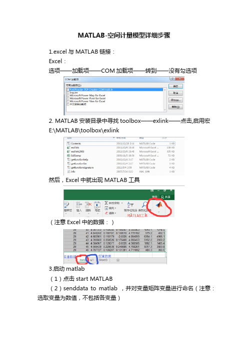
MATLAB-空间计量模型详细步骤1.excel与MATLAB链接:Excel:选项——加载项——COM加载项——转到——没有勾选项2. MATLAB安装目录中寻找toolbox——exlink——点击,启用宏E:\MATLAB\toolbox\exlink然后,Excel中就出现MATLAB工具(注意Excel中的数据:)3.启动matlab(1)点击start MATLAB(2)senddata to matlab ,并对变量矩阵变量进行命名(注意:选取变量为数值,不包括各变量)(data表中数据进行命名)(空间权重进行命名)(3)导入MATLAB中的两个矩阵变量就可以看见4.将elhorst和jplv7两个程序文件夹复制到MATLAB安装目录的toolbox文件夹5.设置路径:6.输入程序,得出结果T=30;N=46;W=norm(W1);y=A(:,3);x=A(:,[4,6]);xconstant=ones(N*T,1); [nobs K]=size(x);results=ols(y,[xconstant x]);vnames=strvcat('logcit','intercept','logp','logy');prt_reg(results,vnames,1);sige=results.sige*((nobs-K)/nobs);loglikols=-nobs/2*log(2*pi*sige)-1/(2*sige)*results.resid'*results.resid % The (robust)LM tests developed by ElhorstLMsarsem_panel(results,W,y,[xconstant x]); % (Robust) LM tests 解释附录:静态面板空间计量经济学一、OLS静态面板编程1、普通面板编程T=30;N=46;W=normw(W1);y=A(:,3);x=A(:,[4,6]);xconstant=ones(N*T,1);[nobs K]=size(x);results=ols(y,[xconstant x]);vnames=strvcat('logcit','intercept','logp','logy');prt_reg(results,vnames,1);sige=results.sige*((nobs-K)/nobs);loglikols=-nobs/2*log(2*pi*sige)-1/(2*sige)*results.resid'*results.resid % The (robust)LM tests developed by ElhorstLMsarsem_panel(results,W,y,[xconstant x]); % (Robust) LM tests2、空间固定OLS (spatial-fixed effects)T=30;N=46;W=normw(W1);y=A(:,3);x=A(:,[4,6]);xconstant=ones(N*T,1);[nobs K]=size(x);model=1;[ywith,xwith,meanny,meannx,meanty,meantx]=demean(y,x, N,T,model );results=ols(ywith,xwith);vnames=strvcat('logcit','logp','logy'); % should be changed if x is changedprt_reg(results,vnames);sfe=meanny-meannx*results.beta; % including the constant term yme = y - mean(y);et=ones(T,1);error=y-kron(et,sfe)-x*results.beta;rsqr1 = error'*error;rsqr2 = yme'*yme;FE_rsqr2 = 1.0 - rsqr1/rsqr2 % r-squared including fixed effectssige=results.sige*((nobs-K)/nobs);logliksfe=-nobs/2*log(2*pi*sige)-1/(2*sige)*results.resid'*results.residLMsarsem_panel(results,W,ywith,xwith); % (Robust) LM tests3、时期固定OLS(time-period fixed effects)T=30;N=46;W=normw(W1);y=A(:,3);x=A(:,[4,6]);xconstant=ones(N*T,1);[nobs K]=size(x);model=2;[ywith,xwith,meanny,meannx,meanty,meantx]=demean(y,x, N,T,model );results=ols(ywith,xwith);vnames=strvcat('logcit','logp','logy'); % should be changed if x is changedprt_reg(results,vnames);tfe=meanty-meantx*results.beta; % including the constant termyme = y - mean(y);en=ones(N,1);error=y-kron(tfe,en)-x*results.beta;rsqr1 = error'*error;rsqr2 = yme'*yme;FE_rsqr2 = 1.0 - rsqr1/rsqr2 % r-squared including fixed effectssige=results.sige*((nobs-K)/nobs);logliktfe=-nobs/2*log(2*pi*sige)-1/(2*sige)*results.resid'*results.residLMsarsem_panel(results,W,ywith,xwith); % (Robust) LM tests4、空间与时间双固定模型T=30;N=46;W=normw(W1);y=A(:,3);x=A(:,[4,6]);xconstant=ones(N*T,1);[nobs K]=size(x);model=3;[ywith,xwith,meanny,meannx,meanty,meantx]=demean(y,x, N,T,model );results=ols(ywith,xwith);vnames=strvcat('logcit','logp','logy'); % should be changed if x is changedprt_reg(results,vnames)en=ones(N,1);et=ones(T,1);intercept=mean(y)-mean(x)*results.beta;sfe=meanny-meannx*results.beta-kron(en,intercept);tfe=meanty-meantx*results.beta-kron(et,intercept);yme = y - mean(y);ent=ones(N*T,1);error=y-kron(tfe,en)-kron(et,sfe)-x*results.beta-kron(ent,intercept); rsqr1 = error'*error;rsqr2 = yme'*yme;FE_rsqr2 = 1.0 - rsqr1/rsqr2 % r-squared including fixed effects sige=results.sige*((nobs-K)/nobs);loglikstfe=-nobs/2*log(2*pi*sige)-1/(2*sige)*results.resid'*results.residLMsarsem_panel(results,W,ywith,xwith); % (Robust) LM tests二、静态面板SAR模型1、无固定效应(No fixed effects)T=30;N=46;W=normw(W1);y=A(:,[3]);x=A(:,[4,6]);for t=1:Tt1=(t-1)*N+1;t2=t*N;wx(t1:t2,:)=W*x(t1:t2,:);endxconstant=ones(N*T,1);[nobs K]=size(x);info.lflag=0;info.model=0;info.fe=0;results=sar_panel_FE(y,[xconstant x],W,T,info); vnames=strvcat('logcit','intercept','logp','logy');prt_spnew(results,vnames,1)% Print out effects estimatesspat_model=0;direct_indirect_effects_estimates(results,W,spat_model); panel_effects_sar(results,vnames,W);2、空间固定效应(Spatial fixed effects)T=30;N=46;W=normw(W1);y=A(:,[3]);x=A(:,[4,6]);for t=1:Tt1=(t-1)*N+1;t2=t*N;wx(t1:t2,:)=W*x(t1:t2,:);endxconstant=ones(N*T,1);[nobs K]=size(x);info.lflag=0;info.model=1;info.fe=0;results=sar_panel_FE(y,x,W,T,info);vnames=strvcat('logcit','logp','logy');prt_spnew(results,vnames,1)% Print out effects estimatesspat_model=0;direct_indirect_effects_estimates(results,W,spat_model);panel_effects_sar(results,vnames,W);3、时点固定效应(Time period fixed effects)T=30;N=46;W=normw(W1);y=A(:,[3]);x=A(:,[4,6]);for t=1:Tt1=(t-1)*N+1;t2=t*N;wx(t1:t2,:)=W*x(t1:t2,:);endxconstant=ones(N*T,1);[nobs K]=size(x);info.lflag=0; % required for exact resultsinfo.model=2;info.fe=0; % Do not print intercept and fixed effects; use info.fe=1 to turn onresults=sar_panel_FE(y,x,W,T,info);vnames=strvcat('logcit','logp','logy');prt_spnew(results,vnames,1)% Print out effects estimatesspat_model=0;direct_indirect_effects_estimates(results,W,spat_model);panel_effects_sar(results,vnames,W);4、双固定效应(Spatial and time period fixed effects)T=30;N=46;W=normw(W1);y=A(:,[3]);x=A(:,[4,6]);for t=1:Tt1=(t-1)*N+1;t2=t*N;wx(t1:t2,:)=W*x(t1:t2,:);endxconstant=ones(N*T,1);[nobs K]=size(x);info.lflag=0; % required for exact resultsinfo.model=3;info.fe=0; % Do not print intercept and fixed effects; use info.fe=1 to turn onresults=sar_panel_FE(y,x,W,T,info);vnames=strvcat('logcit','logp','logy');prt_spnew(results,vnames,1)% Print out effects estimatesspat_model=0;direct_indirect_effects_estimates(results,W,spat_model);panel_effects_sar(results,vnames,W);三、静态面板SDM模型1、无固定效应(No fixed effects)T=30;N=46;W=normw(W1);y=A(:,[3]);x=A(:,[4,6]);for t=1:Tt1=(t-1)*N+1;t2=t*N;wx(t1:t2,:)=W*x(t1:t2,:);endxconstant=ones(N*T,1);[nobs K]=size(x);info.lflag=0;info.model=0;info.fe=0;results=sar_panel_FE(y,[xconstant x wx],W,T,info);vnames=strvcat('logcit','intercept','logp','logy','W*logp','W*l ogy');prt_spnew(results,vnames,1)% Print out effects estimatesspat_model=1;direct_indirect_effects_estimates(results,W,spat_model);panel_effects_sdm(results,vnames,W);2、空间固定效应(Spatial fixed effects)T=30;N=46;W=normw(W1);y=A(:,[3]);x=A(:,[4,6]);for t=1:Tt1=(t-1)*N+1;t2=t*N;wx(t1:t2,:)=W*x(t1:t2,:);endxconstant=ones(N*T,1);[nobs K]=size(x);info.lflag=0; % required for exact resultsinfo.model=1;info.fe=0; % Do not print intercept and fixed effects; use info.fe=1 to turn onresults=sar_panel_FE(y,[x wx],W,T,info);vnames=strvcat('logcit','logp','logy','W*logp','W*logy');prt_spnew(results,vnames,1)% Print out effects estimatesspat_model=1;direct_indirect_effects_estimates(results,W,spat_model);panel_effects_sdm(results,vnames,W);3、时点固定效应(Time period fixed effects)T=30;N=46;W=norm(W1);y=A(:,[3]);x=A(:,[4,6]);for t=1:Tt1=(t-1)*N+1;t2=t*N;wx(t1:t2,:)=W*x(t1:t2,:);endxconstant=ones(N*T,1);[nobs K]=size(x);info.lflag=0; % required for exact resultsinfo.model=2;info.fe=0; % Do not print intercept and fixed effects; use info.fe=1 to turn on% New routines to calculate effects estimatesresults=sar_panel_FE(y,[x wx],W,T,info);vnames=strvcat('logcit','logp','logy','W*logp','W*logy');% Print out coefficient estimatesprt_spnew(results,vnames,1)% Print out effects estimatesspat_model=1;direct_indirect_effects_estimates(results,W,spat_model);panel_effects_sdm(results,vnames,W)4、双固定效应(Spatial and time period fixed effects)T=30;N=46;W=normw(W1);y=A(:,[3]);x=A(:,[4,6]);for t=1:Tt1=(t-1)*N+1;t2=t*N;wx(t1:t2,:)=W*x(t1:t2,:);endxconstant=ones(N*T,1);[nobs K]=size(x);info.bc=0;info.lflag=0; % required for exact resultsinfo.model=3;info.fe=0; % Do not print intercept and fixed effects; use info.fe=1 to turn onresults=sar_panel_FE(y,[x wx],W,T,info);vnames=strvcat('logcit','logp','logy','W*logp','W*logy');prt_spnew(results,vnames,1)% Print out effects estimatesspat_model=1;direct_indirect_effects_estimates(results,W,spat_model);panel_effects_sdm(results,vnames,W)wald test spatial lag% Wald test for spatial Durbin model against spatial lagmodelbtemp=results.parm;varcov=results.cov;Rafg=zeros(K,2*K+2);for k=1:KRafg(k,K+k)=1; % R(1,3)=0 and R(2,4)=0;endWald_spatial_lag=(Rafg*btemp)'*inv(Rafg*varcov*Rafg')*Raf g*btemp prob_spatial_lag=1-chis_cdf (Wald_spatial_lag, K) wald test spatial error% Wald test spatial Durbin model against spatial error model R=zeros(K,1);for k=1:KR(k)=btemp(2*K+1)*btemp(k)+btemp(K+k); % k changed in 1,7/12/2010% R(1)=btemp(5)*btemp(1)+btemp(3);% R(2)=btemp(5)*btemp(2)+btemp(4);endRafg=zeros(K,2*K+2);for k=1:KRafg(k,k) =btemp(2*K+1); % k changed in 1, 7/12/2010Rafg(k,K+k) =1;Rafg(k,2*K+1)=btemp(k);% Rafg(1,1)=btemp(5);Rafg(1,3)=1;Rafg(1,5)=btemp(1);% Rafg(2,2)=btemp(5);Rafg(2,4)=1;Rafg(2,5)=btemp(2);endWald_spatial_error=R'*inv(Rafg*varcov*Rafg')*Rprob_spatial_error=1-chis_cdf (Wald_spatial_error,K)LR test spatial lagresultssar=sar_panel_FE(y,x,W,T,info);LR_spatial_lag=-2*(resultssar.lik-results.lik)prob_spatial_lag=1-chis_cdf (LR_spatial_lag,K)LR test spatial errorresultssem=sem_panel_FE(y,x,W,T,info);LR_spatial_error=-2*(resultssem.lik-results.lik)prob_spatial_error=1-chis_cdf (LR_spatial_error,K)5、空间随机效应与时点固定效应模型T=30;N=46;W=normw(W1);y=A(:,[3]);x=A(:,[4,6]);for t=1:Tt1=(t-1)*N+1;t2=t*N;wx(t1:t2,:)=W*x(t1:t2,:);endxconstant=ones(N*T,1);[nobs K]=size(x);[ywith,xwith,meanny,meannx,meanty,meantx]=demean(y,[x wx],N,T,2); % 2=time dummiesinfo.model=1;results=sar_panel_RE(ywith,xwith,W,T,info);prt_spnew(results,vnames,1)spat_model=1;direct_indirect_effects_estimates(results,W,spat_model);panel_effects_sdm(results,vnames,W)wald test spatial lagbtemp=results.parm(1:2*K+2);varcov=results.cov(1:2*K+2,1:2*K+2);Rafg=zeros(K,2*K+2);for k=1:KRafg(k,K+k)=1; % R(1,3)=0 and R(2,4)=0;endWald_spatial_lag=(Rafg*btemp)'*inv(Rafg*varcov*Rafg')*Raf g*btempprob_spatial_lag= 1-chis_cdf (Wald_spatial_lag, K)wald test spatial errorR=zeros(K,1);for k=1:KR(k)=btemp(2*K+1)*btemp(k)+btemp(K+k); % k changed in 1,7/12/2010% R(1)=btemp(5)*btemp(1)+btemp(3);% R(2)=btemp(5)*btemp(2)+btemp(4);endRafg=zeros(K,2*K+2);for k=1:KRafg(k,k) =btemp(2*K+1); % k changed in 1, 7/12/2010 Rafg(k,K+k) =1;Rafg(k,2*K+1)=btemp(k);% Rafg(1,1)=btemp(5);Rafg(1,3)=1;Rafg(1,5)=btemp(1);% Rafg(2,2)=btemp(5);Rafg(2,4)=1;Rafg(2,5)=btemp(2);endWald_spatial_error=R'*inv(Rafg*varcov*Rafg')*Rprob_spatial_error= 1-chis_cdf (Wald_spatial_error,K)LR test spatial lagresultssar=sar_panel_RE(ywith,xwith(:,1:K),W,T,info);LR_spatial_lag=-2*(resultssar.lik-results.lik)prob_spatial_lag=1-chis_cdf (LR_spatial_lag,K)LR test spatial errorresultssem=sem_panel_RE(ywith,xwith(:,1:K),W,T,info);LR_spatial_error=-2*(resultssem.lik-results.lik)prob_spatial_error=1-chis_cdf (LR_spatial_error,K)四、静态面板SEM模型1、无固定效应(No fixed effects)T=30;N=46;W=normw(W1);y=A(:,[3]);x=A(:,[4,6]);for t=1:Tt1=(t-1)*N+1;t2=t*N;wx(t1:t2,:)=W*x(t1:t2,:);endxconstant=ones(N*T,1);[nobs K]=size(x);info.lflag=0;info.model=0;info.fe=0;results=sem_panel_FE(y,[xconstant x],W,T,info);vnames=strvcat('logcit','intercept','logp','logy');prt_spnew(results,vnames,1)% Print out effects estimatesspat_model=0;direct_indirect_effects_estimates(results,W,spat_model); panel_effects_sar(results,vnames,W);2、空间固定效应(Spatial fixed effects)T=30;N=46;W=normw(W1);y=A(:,[3]);x=A(:,[4,6]);for t=1:Tt1=(t-1)*N+1;t2=t*N;wx(t1:t2,:)=W*x(t1:t2,:);endxconstant=ones(N*T,1);[nobs K]=size(x);info.lflag=0;info.model=1;info.fe=0;results=sem_panel_FE(y,x,W,T,info);vnames=strvcat('logcit','logp','logy');prt_spnew(results,vnames,1)% Print out effects estimatesspat_model=0;direct_indirect_effects_estimates(results,W,spat_model); panel_effects_sar(results,vnames,W);3、时点固定效应(Time period fixed effects)T=30;N=46;W=normw(W1);y=A(:,[3]);x=A(:,[4,6]);for t=1:Tt1=(t-1)*N+1;t2=t*N;wx(t1:t2,:)=W*x(t1:t2,:);endxconstant=ones(N*T,1);[nobs K]=size(x);info.lflag=0; % required for exact resultsinfo.model=2;info.fe=0; % Do not print intercept and fixed effects; use info.fe=1 to turn onresults=sem_panel_FE(y,x,W,T,info);vnames=strvcat('logcit','logp','logy');prt_spnew(results,vnames,1)% Print out effects estimatesspat_model=0;direct_indirect_effects_estimates(results,W,spat_model);panel_effects_sar(results,vnames,W);4、双固定效应(Spatial and time period fixed effects)T=30;N=46;W=normw(W1);y=A(:,[3]);x=A(:,[4,6]);for t=1:Tt1=(t-1)*N+1;t2=t*N;wx(t1:t2,:)=W*x(t1:t2,:);endxconstant=ones(N*T,1);[nobs K]=size(x);info.lflag=0; % required for exact resultsinfo.model=3;info.fe=0; % Do not print intercept and fixed effects; use info.fe=1 to turn onresults=sem_panel_FE(y,x,W,T,info);vnames=strvcat('logcit','logp','logy');prt_spnew(results,vnames,1)% Print out effects estimatesspat_model=0;direct_indirect_effects_estimates(results,W,spat_model); panel_effects_sar(results,vnames,W);五、静态面板SDEM模型1、无固定效应(No fixed effects)T=30;N=46;W=normw(W1);y=A(:,[3]);x=A(:,[4,6]);。
第六讲空间计量经济学基本模型的matlab估计方案

一、Matlab使用前的入数据 第二步:调用函数,函数包含在各专业
工具箱(toolbox)内。 第三步:运行函数,输出结果。
2019/9/10
将专业函数包装入工具箱
第一步:下载专业函数包jplv7,解压。 第二步:装入工具箱(file-setpath)
2019/9/10
二、空间计量基本模型的Matlab估计 函数
一阶空间滞后模型
模型:y=ρwy+e 函数:far 使用方法:res=far(y,w) 例子:p57,example3.1
2019/9/10
空间滞后模型
模型:y=ρwy+xβ+e 函数:sar 使用方法:res=sar(y,x,w) 例子:p66,example3.4
2019/9/10
数据导入matlab
命令:load
文件:.dat格式文件;.ford格式文件 例子:load anselin.dat;load anselin.ford
命令:xlsread
文件:anselin.xls 例子:A=xlsread(anselin.xls)
2019/9/10
2019/9/10
广义空间模型
模型:y=ρw1y+xβ+u, u=λw2u+e 函数:sac 使用方法:res=sac(y,x,w1,w2) 例子:p92,example3.11
2019/9/10
人有了知识,就会具备各种分析能力, 明辨是非的能力。 所以我们要勤恳读书,广泛阅读, 古人说“书中自有黄金屋。 ”通过阅读科技书籍,我们能丰富知识, 培养逻辑思维能力; 通过阅读文学作品,我们能提高文学鉴赏水平, 培养文学情趣; 通过阅读报刊,我们能增长见识,扩大自己的知识面。 有许多书籍还能培养我们的道德情操, 给我们巨大的精神力量, 鼓舞我们前进。
Matlab技术经济学应用
Matlab技术经济学应用引言:技术经济学是一门研究科技创新与经济发展之间相互关系的学科,而Matlab作为一种强大的数值计算和科学编程语言,被广泛应用于技术经济学领域。
本文将重点探讨Matlab在技术经济学中的应用,着重介绍其在经济评估、金融模型、企业决策等方面的应用。
一、经济评估1.1 投资成本分析在进行经济评估时,投资成本分析是一个重要的步骤。
Matlab可以帮助分析人员通过数学模型计算出投资成本,并进行灵活的调整和优化。
例如,可以使用Matlab编写一个程序,基于现金流量贴现法(NPV)来计算投资项目的净现值。
通过调整输入参数,可以模拟不同情况下的投资成本,并找到最优方案。
1.2 效益评估Matlab也可以用于效益评估,即对投资项目的经济效益进行分析。
例如,可以使用Matlab编写一个程序来计算投资项目的内部收益率(IRR),并评估其可行性和盈利能力。
通过在程序中引入不同的输入变量,可以进行灵活的模拟和分析,帮助决策者做出科学的投资决策。
二、金融模型2.1 期权定价模型期权定价是金融领域中的一个重要问题,Matlab提供了强大的数学计算功能,可以用于构建和求解各种期权定价模型。
例如,可以使用Matlab编写程序,基于布莱克-斯科尔斯(Black-Scholes)模型来估计欧式期权的价格。
通过调整输入参数,可以对不同情况下的期权价格进行计算和分析。
2.2 风险管理模型金融市场中存在着各种风险,如市场风险、信用风险等。
Matlab可以用于构建和求解各种风险管理模型,以帮助投资者进行风险评估和管理。
例如,可以使用Matlab编写程序,基于Value at Risk(VaR)模型来评估投资组合的风险水平,并制定相应的风险管理策略。
三、企业决策3.1 供应链优化供应链管理是现代企业中的一个重要问题,而Matlab可以帮助企业进行供应链优化。
例如,可以使用Matlab编写程序,基于线性规划模型来优化供应链网络的布局和物流运输方案。
在Matlab中进行模型建立和参数估计
在Matlab中进行模型建立和参数估计引言在科学研究和工程实践中,建立数学模型并通过参数估计对模型进行优化是常见的任务。
Matlab作为一种功能强大的数学计算工具,提供了丰富的函数和工具箱,可以方便地进行模型建立和参数估计。
本文将介绍在Matlab中进行模型建立和参数估计的基本方法和技巧。
一、模型建立模型建立是构建一个能够描述实际问题的数学模型的过程。
在Matlab中,可以使用符号运算工具箱(Symbolic Math Toolbox)来定义符号变量和代数表达式,并利用这些符号变量和代数表达式构建模型。
例如,对于线性回归模型,可以使用符号变量定义输入变量和待估参数,并通过代数表达式构建模型方程。
除了使用符号运算工具箱,Matlab还提供了许多其他工具箱和函数来进行模型建立。
例如,Curve Fitting Toolbox可以用于拟合曲线和表面,System Identification Toolbox可以用于系统建模和参数估计等。
这些工具箱和函数提供了丰富的方法和算法来支持各种类型的模型建立。
二、参数估计参数估计是通过观测数据来估计模型中的未知参数的过程。
在Matlab中,可以使用最小二乘法(Least Squares)或最大似然估计(Maximum Likelihood Estimation)等方法进行参数估计。
最小二乘法是一种常用的参数估计方法,通过最小化观测数据与模型预测值之间的误差平方和来估计参数。
在Matlab中,可以使用lsqcurvefit函数或最小二乘曲线拟合工具箱(Curve Fitting Toolbox)中的相关函数来进行最小二乘估计。
这些函数可以根据用户提供的模型函数、初始参数值和观测数据进行参数估计,并返回估计的参数值和相应的拟合误差等信息。
最大似然估计是一种统计推断方法,通过估计参数使得观测数据的出现概率最大化。
在Matlab中,可以使用mle函数或Probability Distribution Fitting工具箱中的相关函数进行最大似然估计。
matlab中ma参数估计
matlab中ma参数估计Estimating parameters in a moving average (MA) model in Matlab can be a complex but essential task in time series analysis. The MA model is commonly used to represent the stochastic process of a time series, with random noise being incorporated into the model through the MA parameters. By accurately estimating these parameters, analysts can better understand and predict the behavior of the time series data.在Matlab中估计移动平均(MA)模型中的参数可能是时间序列分析中一个复杂但必要的任务。
MA模型通常用于表示时间序列的随机过程,通过MA参数将随机噪声纳入模型中。
通过准确估计这些参数,分析师可以更好地了解和预测时间序列数据的行为。
One way to estimate MA parameters in Matlab is through maximum likelihood estimation. This method involves finding the values of the MA parameters that maximize the likelihood function, which measures how well the model explains the observed data. By iteratively adjusting the parameter values to maximize the likelihood, analysts can arrive at estimates that best fit the data.在Matlab中估计MA参数的一种方法是通过最大似然估计。
7.3 空间计量经济学模型的估计与检验

b [X 'Ω 1 X ] 1 X 'Ω 1 A Y
b [ X 'Ω 1 X ] 1 X 'Ω 1 Y [ X 'Ω 1 X ] 1 X 'Ω 1 W Y
YXβ1 ε (1) WYXβ2 ε (2)
b1[X'Ω1X]1X'Ω1Y b2[X'Ω1X]1X'Ω1WY
• 由于事先无法根据先验经验判断这些假设的真伪, 有必要构建一种判别准则,以决定哪种空间模型更 加符合客观实际。
第二十五页,编辑于星期五:十点 五十五分。
• 判别准则:
– 如果在空间效应的检验中发现LMLAG较之LMERR在统计上 更加显著,且R-LMLAG显著而R-LMERR不显著,则可以 断定适合的模型是空间滞后模型;
相关;(统计量称为LMERR ) – 检验2是在存在空间自回归的假设下检验是否存在空间
残差相关;(统计量称为R-LMERR) – 检验3是在不存在空间残差相关的假设下检验是否存在空
间自回归效应;(统计量称为LMLAG) – 检验4是在存在空间残差相关的假设下检验是否存在空
间自回归效应。(统计量称为R-LMLAG )
22
2
N l n 2 1 l n { |Ω |* [ |B |] 2 } 1 [ B Y B X β ] 'Ω 1 [ B Y B X β ] 1
22
2
2
0
s21e'e,Ttr(W 'W W 2) N
1
2
e' We
LM(e'Wes2)2 ~2(1)
T
第十六页,编辑于星期五:十点 五十五分。
- 1、下载文档前请自行甄别文档内容的完整性,平台不提供额外的编辑、内容补充、找答案等附加服务。
- 2、"仅部分预览"的文档,不可在线预览部分如存在完整性等问题,可反馈申请退款(可完整预览的文档不适用该条件!)。
- 3、如文档侵犯您的权益,请联系客服反馈,我们会尽快为您处理(人工客服工作时间:9:00-18:30)。
info为结构化参数,事前赋值;
通常调整info.lflag(标准n?1000)、info.rmin和info.rmax。
***********************************************************
3)vnames
在输出结果中说明被解释变量。
使用方法:
res:存储结果的变量;
y:被解释变量;
x:解释变量;
w:空间权重矩阵;
info:结构化参数,具体可使用
helpsar
语句查看
====================================================
注意事项
1)W
W为权重矩阵,因为是稀疏矩阵,原始数据通常以n×3的数组形式存储,需要用sparse函数转换为矩阵形式。
使用方法:
[W1W2 W3]=xy2cont(x,y)
其中,W2是行标准化后的空间邻接矩阵。
一个例子:
使用anselin数据,生成w,并与wmat比较其差异。
====================================================
二、空间误差模型
sem()
====================================================
***********************************************************
5)vnames
在输出结果中说明被解释变量。
使用方法:
vnames=strvcat(‘variablename1’,’variablename2’……);
***********************************************************
第七讲-空间计量经济学模型的matlab估计
———————————————————————————————— 作者:
——————————————————————————经济学基本模型的matlab估计
一、空间滞后模型
sar()
====================================================
可以通过matlab软件打开elect.dat查看,并打开elect.txt查看各列数据的含义。
计量模型
认为各县的投票率受到相邻地区投票率的影响,同时,还受到选民教育水平、选民住房情况、选民收入水平的影响,据此得到如下计量模型:
y=β0+ρWy+xβ+ε
ε~N(0,σ2In)
转换为:
y=ρWy+[1x][β0β]’+ε
函数功能
估计空间误差模型
中的未知参数β、λ和σ2。
====================================================
使用方法
res=sem(y,x,W,info)
***********************************************************
6)Asymptotict-stat(渐进t统计量)
rho的检验:渐进t分布,估计值的显著性使用相应的Z概率表示。
====================================================
应用实例
估计地区投票率受周边地区投票率的影响程度
案例素材
1997年,Pace等人研究了美国3107个县的选举投票率影响因素,运用的是美国1980年大选的公开投票数据,形成了一个包含3107个样本数据的截面数据集elect.dat。
res:存储结果的变量;
y:被解释变量;
x:解释变量;
w:空间权重矩阵;
info:结构化参数,具体可使用
helpsem
语句查看
====================================================
注意事项
1)x
x应将常数项包括在内。
***********************************************************
3)x
需要注意x的生成方式,应将常数项包括在内。
***********************************************************
4)info
info为结构化参数,事前赋值;
通常调整info.lflag(标准n?1000)、info.rmin和info.rmax。
应用实例
估计地区投票率受周边地区投票率的影响程度
案例素材
1997年,Pace等人研究了美国3107个县的选举投票率影响因素,运用的是美国1980年大选的公开投票数据,形成了一个包含3107个样本数据的截面数据集elect.dat。
vnames=strvcat(‘variable name1’,’variablename2’……);
***********************************************************
====================================================
ε~N(0,σ2In)
程序语句
1)近似估计
缺省设置:info.lflag=1
注意取对数值,得到y,x。
2)精确估计
info.lflag=0
运行结果
====================================================
xy2cont()
函数功能:
使用地区x坐标和y坐标,生成空间邻接矩阵。
函数功能
估计空间滞后模型(空间自回归-回归模型)
中的未知参数ρ、β和σ2。
====================================================
使用方法
res=sar(y,x,W,info)
***********************************************************
***********************************************************
2)ydev(不再需要)
sar函数求解的标准模型可以包含常数项,被解释变量(因变量)y,不再需要转换为离差形式(ydev)。
***********************************************************