Processing k-skyband, constrained skyline, and group-by skyline queries on incomplete data

合集下载

mintpy的处理结果

mintpy的处理结果英文回答：Mintpy is a powerful tool for processing and analyzing interferometric synthetic aperture radar (InSAR) data. Itis specifically designed for studying surface deformation caused by various geophysical processes such as earthquakes, volcanoes, and land subsidence. Mintpy provides a widerange of functionalities, including data processing, time series analysis, and visualization, making it a valuabletool for geoscientists and researchers.One of the key features of Mintpy is its ability to process large datasets efficiently. It can handle data from multiple radar satellites, such as Sentinel-1 and ALOS-2, and can process data from different acquisition modes, including ascending and descending orbits. This allowsusers to analyze long time series of InSAR data and extract valuable information about the Earth's surface deformation.Mintpy also offers a variety of processing algorithms, including phase unwrapping, baseline estimation, and atmospheric correction. These algorithms help to improve the quality of the InSAR data and reduce noise and artifacts. Additionally, Mintpy provides advanced time series analysis tools, such as the Small Baseline Subset (SBAS) and the Temporal StaMPS (TStaMPS) algorithms, which allow users to detect and monitor subtle surface deformation over time.Furthermore, Mintpy has a user-friendly interface that allows users to easily navigate through the different processing steps and visualize the results. It provides interactive plotting tools for visualizing interferograms, coherence maps, and time series plots. Users can also export the results in various formats, such as GeoTIFF and KMZ, for further analysis or visualization in other software.Overall, Mintpy is a versatile and efficient tool for processing and analyzing InSAR data. Its wide range of functionalities, efficient processing algorithms, and user-friendly interface make it a valuable asset for researchers and geoscientists studying surface deformation.中文回答：Mintpy是一款用于处理和分析干涉合成孔径雷达（InSAR）数据的强大工具。

gfcanalysis包：Hansen等全球森林变化数据集工具说明书

Package‘gfcanalysis’October11,2023Version1.8.0Date2023-10-09Language en-usTitle Tools for Working with Hansen et al.Global Forest ChangeDatasetDepends R(>=3.5.0),raster,methodsImports sf,terra,geosphere,RCurl,plyr,ggplot2,grid,stringr,animation,rasterVisEncoding UTF-8Description Supports analyses using the Global Forest Change dataset released by Hansen et al.gfcanalysis was originally written for the Tropical Ecology Assessment and Monitoring(TEAM)Network.For additional details on the Global Forest Change dataset,see:Hansen,M.et al.2013.``High-Resolution Global Maps of21st-Century Forest Cover Change.''Science342(15November):850-53.The forest change data and more information on theproduct is available at<>. License GPL(>=3)URL https:///azvoleff/gfcanalysisBugReports https:///azvoleff/gfcanalysis/issues LazyData trueRoxygenNote7.2.3NeedsCompilation noAuthor Alex Zvoleff[aut],Matthew Cooper[cre]Maintainer Matthew Cooper<*******************>Repository CRANDate/Publication2023-10-1112:20:02UTC12animate_annual R topics documented:animate_annual (2)annual_stack (3)calc_gfc_tiles (4)calc_pixel_areas (5)check_aoi (5)download_tiles (6)extract_gfc (7)gfc_stats (8)gfc_tiles (9)plot_gfc (9)scale_by_pixel_area (10)scale_toar (10)test_poly (11)threshold_gfc (11)utm_zone (13)Index15 animate_annual Plot an animation of forest change within a given area of interest(AOI)DescriptionProduces an animation of annual forest change in the area bounded by the extent of a given AOI,or AOIs.The AOI polygon(s)is(are)also plotted on the image.The gfc_stack must be pre-calculated using the annual_stack function.The animation can be either an animated GIF(if type is set to ’gif’)or a series of’.png’ﬁles with a corresponding’.html’webpage showing a simple viewer and the forest change animation(if type is set to’html’).The HTML option is recommended as it requires no additional software to produce it.The animated GIF option will only work if the imagemagicK software package is installed beforehand(this is done outside of R).Usageanimate_annual(aoi,gfc_stack,out_dir=getwd(),out_basename="gfc_animation",site_name="",type="html",height=3,width=3,dpi=300,dataset="GFC-2022-v1.10")annual_stack3Argumentsaoi one or more AOI polygons as a SpatialPolygonsDataFrame or sf object.If there is a’label’ﬁeld in the dataframe,it will be used to label the polygons inthe plots.If the AOI is not in the WGS84geographic coordinate system,it willbe reprojected to WGS84.gfc_stack a GFC product subset as a RasterStack(as output by annual_stack)out_dir folder for animation outputout_basename basename to use when naming animationﬁlessite_name name of the site(used in making title)type type of animation to make.Can be either"gif"or"html"height desired height of the animation GIF in incheswidth desired width of the animation GIF in inchesdpi dots per inch for the output imagedataset which version of the Hansen data to use annual_stack was runSee Alsoannual_stackannual_stack Generate an annual stack of forest change from GFC productDescriptionUses thresholded GFC data as output by threshold_gfc to make an annualized layer stack of forest change.See Details for the class codes used in the annual raster stack.The animate_annual function can be used to produce an animation of forest change from the generated layer stack.Usageannual_stack(gfc,dataset="GFC-2022-v1.10")Argumentsgfc thresholded extract of GFC product for a given AOI(see threshold_gfc) dataset which version of the Hansen data to use4calc_gfc_tilesDetailsThe output raster stack uses the following codes to describe forest change at each pixel:Nodata0Forest1Non-forest2Forest loss3Forest gain4Forest loss and gain5Water6See Alsothreshold_gfc,animate_annualcalc_gfc_tiles Calculate the GFC product tiles needed for a given AOIDescriptionIntersects an AOI with the GFC product grid to determine what tiles are need to cover the AOI.Usagecalc_gfc_tiles(aoi)Argumentsaoi an Area of Interest(AOI)as a SpatialPolygons*or sf object.If the AOI is not in the WGS84geographic coordinate system,it will be reprojected to WGS84.Valuea sf of the GFC tiles needed to cover the AOIExamplestiles<-calc_gfc_tiles(test_poly)plot(tiles)plot(test_poly,lt=2,add=TRUE)calc_pixel_areas5 calc_pixel_areas Calculates the pixel area for each line of a rasterDescriptionCalculates the pixel area for each line of a rasterUsagecalc_pixel_areas(x)Argumentsx a Raster*objectValuea vector with the area in square meters of the pixels in each line of x(vector has length equal tonrow(x))check_aoi Check if aoi is an sf or sp type object If sp,convert to sf and returnDescriptionCheck if aoi is an sf or sp type object If sp,convert to sf and returnUsagecheck_aoi(aoi)Argumentsaoi the area of interest object6download_tiles download_tiles Download a set of GFC tilesDescriptionThis functionﬁrst checks whether each tile in a set GFC product tiles is present locally,and that localﬁle sizes match theﬁle sizes of theﬁles available on the Google server hosting the GFC product.Next,the function downloads all tiles that either are not present locally,or that are present but haveﬁle sizes differing from theﬁle on the Google server.Usagedownload_tiles(tiles,output_folder,images=c("treecover2000","lossyear","gain","datamask"),dataset="GFC-2022-v1.10")Argumentstiles sf with GFC product tiles to download,as calculated by the calc_gfc_tilesfunction.output_folder the folder to save output data inimages which images to download.Can be any of’treecover2000’,’loss’,’gain’,’lossyear’,’datamask’,’ﬁrst’,and’last’.dataset which version of the Hansen data to useSee Alsoextract_gfcExamples##Not run:output_folder<- H:/Data/TEAM/GFC_Producttiles<-calc_gfc_tiles(test_poly)download_tiles(tiles,output_folder)##End(Not run)extract_gfc7 extract_gfc Extracts GFC data for a given AOIDescriptionThis function extracts a dataset for a given AOI from a series of pre-downloaded GFC tiles.The download_tiles function should be used beforehand in order to download the necessary data to the speciﬁed data_folder.Note that the outputﬁle format isﬁxed as GeoTIFF with LZW com-pression.Usageextract_gfc(aoi,data_folder,to_UTM=FALSE,stack="change",dataset="GFC-2022-v1.10",...)Argumentsaoi an Area of Interest(AOI)as a sf object.If the AOI is not in WGS1984 (EPSG:4326),it will be reprojected to WGS84.data_folder folder where downloaded GFC product tiles are located(see download_tiles function.to_UTM if TRUE,then reproject the output into the UTM zone of the AOI centroid.If FALSE,retain the original WGS84projection of the GFC tiles.stack the layers to extract from the GFC product.Defaults to"change".See Details.dataset which version of the Hansen data to use...additional arguments as for writeRaster,such as filename,or overwrite. DetailsThe stack option can be"change"(the default),"ﬁrst",or"last".When set to"change",the forest change layers(treecover2000,loss,gain,lossyear,and datamask)will be extracted for the given aoi.The"ﬁrst"and"last"options will mosaic the2000or last year composite top of atmosphere (TOA)reﬂectance images(respectively).ValueRasterStack with GFC layersSee Alsodownload_tiles,annual_stack,gfc_stats8gfc_stats gfc_stats Produce a table of forest cover change statistics for a given AOIDescriptionFor a given AOI,this function produces two tables:an annual forest loss table(in hectares,by default),and a table specifying1)the total area of pixels that experienced forest gain and,2)the total area of pixels that experienced both loss and gain over the full period(from2000through the end date of the speciﬁc product you are using,depending on the chosen dataset).Note that forest gain and combined loss and gain are not available in the GFC product on an annualized e extract_gfc to extract the GFC data for the AOI,and threshold it using threshold_gfc prior to running this function.Usagegfc_stats(aoi,gfc,scale_factor=1e-04,dataset="GFC-2022-v1.10") Argumentsaoi one or more Area of Interest(AOI)polygon(s)as a SpatialPolygons*.See Details.gfc extract of GFC product for a given AOI(see extract_gfc),recoded using threshold_gfc.scale_factor how to scale the output data(from meters).Defaults to.0001for output in hectares.dataset which version of the Hansen data to useDetailsIf the aoi object is not in the coordinate system of gfc,it will be reprojected.If there is a"label"attribute,it will be used to label the output statistics.Otherwise,unique names("AOI1","AOI2", etc.)will be generated and used to label the output.If multiple AOIs share the same labels,statistics will be provided for the union of these AOIs.Valuelist with two elements"loss_table",a data.frame with statistics on forest loss,and"gain_table", with the area of forest gain,and area that experienced both loss and gain.The units of the output are hectares(when scale_factor is set to.0001).See Alsoextract_gfc,threshold_gfcgfc_tiles9 gfc_tiles Grid of tiles used for the GFC productDescriptionContains a SpatialPolygonsDataFrame with a10x10degree grid in WGS84coordinate system, covering the area from180W-180E and80N-60S,the tile system used by the GFC Product.plot_gfc Plot forest change(relative to2000)for a given yearDescriptionPlots a single layer of forest change from a layer stack output by annual_stack.Usageplot_gfc(fchg,aoi,title_string="",size_scale=1,maxpixels=50000)Argumentsfchg a forest change raster layer(a single layer of the layer stack output by annual_stack aoi one or more AOI polygons as a SpatialPolygonsDataFrame or sf object.Ifthere is a’label’ﬁeld in the dataframe,it will be used to label the polygons inthe plots.If the AOI is not in WGS1984(EPSG:4326),it will be reprojected toWGS84.title_string the plot titlesize_scale a number used to scale the size of the plot textmaxpixels the maximum number of pixels from fchg to use in plottingSee Alsoannual_stack,animate_annual10scale_toar scale_by_pixel_area Scales a raster by the area of each pixel in metersDescriptionCalculates the area(in meters)of each pixel in a raster,scales the value of each pixel by the area, applies the desired scale factor,and returns the result as a eful for calculating class areas based on a classiﬁed raster in a geographic coordinate system.Assumes that raster is not rotated(latitudes of every pixel in a given row are identical).Processes block by block to support handling very large rasters.Usagescale_by_pixel_area(x,filename,datatype,pixel_areas=NULL,scale_factor=1)Argumentsx a Raster*objectfilename(optional)ﬁlename for output rasterdatatype(optional)datatype for output raster see dataType NOT YET SUPPORTED pixel_areas a vector giving the area of each cell in a single column of the raster.See calc_pixel_areas.If NULL,this vector will be calculated based on the coor-dinate system of x.scale_factor a value to scale the results byValueRasterLayer with pixel areas(in meters)scale_toar Scale theﬁrst or last top of atmosphere(TOA)reﬂectance imagesDescriptionThis function applies the scale factors provided by Hansen et al.to rescale theﬁrst and last TOA reﬂectance images from integer toﬂoating point.The following scale factors are used:band3,508;band4,254;band5,363;band7,423.The output datatype is FLT4S.test_poly11Usagescale_toar(x,...)Argumentsx the"ﬁrst"or"last"image for a given aoi as a RasterStack(see stack option for extract_gfc)....additional arguments as for writeRaster,such as filename,or overwrite. ValueRasterStack of TOA reﬂectance valuesSee Alsoextract_gfctest_poly Polygon outlining TEAM site in Caxiuanã,BrazilDescriptionContains a SpatialPolygonsDataFrame with a simpliﬁed polygon of the area within the Tropical Ecology Assessment and Monitoring(TEAM)network site in Caxiuanã,Brazil.threshold_gfc Threshold the GFC productDescriptionUses the GFC data output from extract_gfc to make an thresholded layer stack withﬁve layers: treecover2000,loss,gain,lossyear,and datamask layers.See Details for the coding used in each layer.Note that the outputﬁle format isﬁxed as GeoTIFF with LZW compression.Usagethreshold_gfc(gfc,forest_threshold=25,...)Argumentsgfc extract of GFC product for a given AOI(see extract_gfc)forest_thresholdpercent woody vegetation to use as a threshold for mapping forest/non-forest ...additional arguments as for writeRaster,such as filename or overwrite12threshold_gfcDetailsThe output uses the following codes to describe forest change at each pixel:Band1(forest2000)Non-forest0Forest1Band2(lossyear)No loss0Loss in20011Loss in20022Loss in20033Loss in20044Loss in20055Loss in20066Loss in20077Loss in20088Loss in20099Loss in201010Loss in201111Loss in201212Loss in201313Loss in201414Note that lossyear is zero for pixels that were not forested in2000,and that the2013and2014loss layers are not available in the original2013Hansen dataset(the2013loss layer is available in the 2014and2015updates,while the2014loss layer is available in the2015update only).Band3(gain)No gain0Gain1Note that gain is zero for pixels that were forested in2000Band4(lossgain)No loss and gain0Loss and gain1Note that loss and gain is difﬁcult to interpret from the thresholded product,as the original GFC product does not provide information on the sequence(loss then gain,or gain then loss),or the levels of canopy cover reached prior to loss(for gain then loss)or after loss(for loss then gainpixels).The layer is calculated here as:lossgain<-gain&(lossyear!=0),where loss year and gain are the original GFC gain and lossyear layers,respectively.Band5(datamask)No data0Land1Water2ValueRasterBrick with thresholded GFC product(see details above)See Alsoextract_gfcutm_zone Given a spatial object,calculate the UTM zone of the centroidDescriptionFor a line or polygon,the UTM zone of the centroid is given,after reprojecting the object into WGS-84.Usageutm_zone(x,y,proj4string=FALSE)##S4method for signature numeric,numericutm_zone(x,y,proj4string=FALSE)##S4method for signature Spatial,missingutm_zone(x,proj4string)Argumentsx a longitude(with western hemisphere longitudes negative),or a Spatial object y a latitude(with southern hemisphere latitudes negative),or missing(if x is a Spatial object)proj4string if FALSE(default)return the UTM zone as a string(for example"34S"for UTM Zone34South).If TRUE,return a proj4string using the EPSG code as aninitialization string.DetailsBased on the code on at http://bit.ly/17SdcuN.Examplesutm_zone(45,10)utm_zone(45,-10)utm_zone(45,10,proj4string=TRUE)Indexanimate_annual,2,3,4,9annual_stack,2,3,3,7,9calc_gfc_tiles,4calc_pixel_areas,5,10check_aoi,5dataType,10download_tiles,6,7extract_gfc,6,7,8,11,13gfc_stats,7,8gfc_tiles,9plot_gfc,9scale_by_pixel_area,10scale_toar,10test_poly,11threshold_gfc,3,4,8,11utm_zone,13utm_zone,numeric,numeric,logical-method(utm_zone),13utm_zone,numeric,numeric-method(utm_zone),13utm_zone,Spatial,missing,logical-method(utm_zone),13utm_zone,Spatial,missing-method(utm_zone),13writeRaster,7,1115。

ERA5资料在蓟州复杂地形下的检验与应用

第４４卷第１期
海洋气象学报
ＪＯＵＲＮＡＬＯＦＭＡＲＩＮＥＭＥＴＥＯＲＯＬＯＧＹ
２０２４年２月
Ｖｏｌ.４４Ｎｏ.１
Ｆｅｂ.ꎬ ２０２４
邹双泽ꎬ白爱娟ꎬ何科ꎬ等.ＥＲＡ５资料在蓟州复杂地形下的检验与应用[ Ｊ] .海洋气象学报ꎬ２０２４ꎬ４４(１) :１１８￣１２８.
ｃａｎｒｅｆｌｅｃｔｔｈｅｃｈａｎｇｅｏｆｗｅａｔｈｅｒａｎｄｐｒｏｖｉｄｅｒｅｆｅｒｅｎｃｅｆｏｒａｎａｌｙｚｉｎｇｓｔｒｏｎｇｃｏｎｖｅｃｔｉｖｅｐｏｔｅｎｔｉａｌ.
ＫｅｙｗｏｒｄｓＪｉｚｈｏｕꎻ Ｄａｘｉｎｇｓｏｕｎｄｉｎｇｓｔａｔｉｏｎꎻ ＥＣＭＷＦＲｅａｎａｌｙｓｉｓｖ５ ( ＥＲＡ５ ) ꎻ ａｅｒｉａｌｅｘｐｌｏｒａｔｉｏｎꎻ
发展专项( ＣＸＦＺ２０２２Ｊ０１２)
第一作者简介:邹双泽ꎬ女ꎬ硕士ꎬ工程师ꎬ主要从事灾害性天气监测预警研究ꎬ３１７９７３１３３＠ｑｑ.ｃｏｍꎮ
通信作者简介:白爱娟ꎬ女ꎬ博士ꎬ教授ꎬ主要从事天气动力学研究ꎬｂａｉａｊ＠ｃｕｉｔ.ｅｄｕ.ｃｎꎮ
第１期
邹双泽等:ＥＲＡ５资料在蓟州复杂地形下的检验与应用
难ꎮ 又如河南郑州“７２０” 特大暴雨[４－５] ꎬ造成全市
需要验证ꎮ
暴雨[１－３] ꎬ引发的城市内涝和山区泥石流造成７８人遇
３８０人因灾死亡或失踪ꎮ 在特定天气形势和环境条
得到广泛应用[１６] ꎬ但在复杂地形区资料的可靠性仍
一方面ꎬ处于复杂地形的天津蓟州短时强降水
件下产生的强对流天气是短时临近预报的重难点ꎬ高
ｓｔｒｏｎｇｃｏｎｖｅｃｔｉｖｅｉｎｄｅｘ
辨率高的优点ꎬ能够提供对流层各高度层的温度、湿

空间数据分析实战Python中的空间数据处理与可视化技术

空间数据分析实战Python中的空间数据处理与可视化技术在当今数字化时代，空间数据的应用越来越广泛，而Python作为一种强大的编程语言，为空间数据的处理和可视化提供了丰富的工具和库。

本文将介绍在Python环境下，如何进行空间数据的处理和可视化，以及相关的实战应用。

1. **空间数据处理基础**在开始之前，首先需要了解空间数据处理的基础知识。

空间数据通常包括地理信息系统（GIS）数据和遥感数据。

GIS数据主要是地理信息的向量数据，如点、线、面等，而遥感数据则是通过遥感技术获取的地表信息，如卫星影像等。

Python中常用的空间数据处理库包括GeoPandas、Shapely和Fiona等，它们提供了丰富的功能来处理和分析空间数据。

2. **空间数据处理实践**接下来，我们将介绍一些常见的空间数据处理实践。

首先是空间数据的读取与展示。

使用GeoPandas可以方便地读取各种格式的空间数据，如Shapefile、GeoJSON等，并且可以通过Matplotlib或其他可视化库将空间数据进行展示，以便进一步分析。

其次是空间数据的空间关系分析。

通过Shapely库，我们可以轻松计算空间对象之间的空间关系，如相交、包含等，从而进行空间数据的拓扑分析和空间查询。

最后是空间数据的地理处理。

Fiona库提供了对各种GIS数据格式的读写功能，使得我们可以对空间数据进行增删改查等地理处理操作，例如数据投影转换、空间缓冲区分析等。

3. **空间数据可视化技术**空间数据可视化是理解和传播空间信息的重要手段。

除了基本的地图展示外，Python中还有一些强大的空间数据可视化库，如Basemap、Cartopy和Plotly等。

这些库不仅可以绘制静态地图，还可以创建交互式地图，使得用户可以通过交互方式探索空间数据，提高数据的可理解性和可交互性。

4. **空间数据分析与可视化实战**最后，我们将介绍一些空间数据分析与可视化的实战案例。

高分二号PMS数据进行完整的预处理流程

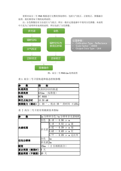
需要对高分二号PMS数据进行完整的预处理时，包括大气校正、正射校正、图像融合处理，我们推荐如下图的处理流程。

注：全色图像没有方法进行大气校正，所以一般在定量遥感中不使用全色图像。

本流程中只是为了说明所有处理的流程，所以包括了全色图像。

图：高分二号PMS L1a处理流程表1 高分二号卫星轨道和姿态控制参数表 2 高分二号卫星有效载荷技术指标1. 数据打开ENVI5.1 暂不支持 GF2 数据 .xml 打开方式，但 GF2 数据为标准 TIFF 格式，故可直接使用 ENVI 的 Open 菜单打开，只是打开后软件不能自动识别元数据信息。

图标，弹出Open 对话框，选启动ENVI5.2 ；依次File > Open 或直接单击工具栏上的择数据文件夹下扩展为.tiff 的文件，然后点击Open 按钮打开（本例中为…/GF2_PMS2_E115.7_N42.7_20140928_L1A0000362235-MSS2.tiff ）。

辐射定标全色图像没有方法进行大气校正，所以一般在定量遥感中不使用全色图像；这里也仅对多光谱数据进行辐射定标。

使用 ENVI 提供的 Apply Gain and Offset 工具进行辐射定标。

（ 1 ）在 Toolbox 中，依次 Radiometric Correction > Apply Gain and Offset ，弹出 Gain and Offset Input File 对话框，在 Select Input File 选项卡中选择待处理影像GF2_PMS2_E115.7_N42.7_20140928_L1A0000362235-MSS2.tiff ，点击 OK ；（ 2 ）弹出 Gain and Offset Values 对话框，依次填入 Gain Values 和 Offset Values ，设置输出路径、文件名及数据类型；（ 3 ）点击 OK 开始执行（图 1 ）。

Origin7.5实用教程_周剑平_色谱峰

（1）AreaFit（Fitted peak area），使用拟合的函数及参数，计算峰与基线之间的积分值，积分区间为–∞~∞；
（2）AreaFitT（Fitted peak area contained in fitting range），使用拟合的函数及参数，计算峰与基线之间的积分值，积分区间为选择的数据范围；
Rs
=
X c2 − X c1 0.5(w2 + w1)
；
（14）Moment3/ Moment4（3rd/4th order moments），3阶和4阶矩，即m3和m4；
（15）WidthAtP（Width at n% of peak maximum），峰最大值n%处的宽度；
（16）AreaAbove（Area above n% of peak maximum），峰最大值n%以上部分的面积；
第9章非线性拟合
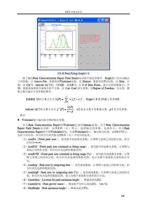
图9.36 Peak Fitting Graph结果
除了输出Peak Characterization Report Field Details对话框中指定参数外，Graph窗口还自动输出下列参数：① Source File，数据组的Worksheet名称；② Dataset，数据组的Y列名称；③ Date，日期；④ Chi^2，reduced chi^2值；⑤COD，系数R^2；⑥ # of Data Points，拟合过程的数据点；⑦ SS，数据曲线和拟合曲线差的平方和；⑧ Corr Coef 相关系数；⑨Degree of Freedom，自由度，数据点数目减去可变参数的数目。
单击Fitting Function Parameters组中的Worksheet按钮，将拟合函数的参数输出到Worksheet，如图9.38所示，包括参数名称、拟合结果、拟合标准差、依赖关系和置信区间。

modis数据时间序列重建代码

modis数据时间序列重建代码如何使用MODIS 数据进行时间序列重建的问题。

MODIS (Moderate Resolution Imaging Spectroradiometer) 数据是由美国国家航空航天局(NASA) 在2000 年发射的Terra 和Aqua 卫星上收集的重要地球观测数据。

这些数据用于监测全球的植被生长、大气成分、海洋表面温度等多种环境参数。

其中，时间序列重建是一种重要的数据分析技术，可以揭示出地球上不同地区的环境变化趋势。

在本文中，我们将介绍如何使用MODIS 数据进行时间序列重建，并提供相应的Python 代码示例来帮助读者更好地理解。

以下是具体的步骤：1. 数据获取：首先，我们需要获取MODIS 数据。

NASA 提供了一系列的数据访问系统，如Earthdata、LAADS 和LPDAAC，用于从Terra 和Aqua 卫星获取MODIS 数据。

根据具体需求，我们可以选择下载不同的产品，比如地表温度、植被指数等。

以MOD13Q1，即植被指数产品为例，我们可以通过访问LPDAAC 网站来获取该产品的数据。

2. 数据预处理：获取到MODIS 数据后，我们需要进行一些预处理步骤来准备数据进行时间序列重建。

首先，我们需要对数据进行筛选，选择我们感兴趣的地点或区域。

接下来，我们需要对数据进行空间插值，填补由于云覆盖等原因产生的缺失值。

最后，我们需要对数据进行时间插值，填补由于卫星轨道或其它原因导致的数据缺失。

3. 时间序列重建模型选择：选择适合的时间序列重建模型是一个关键的步骤。

根据MODIS 数据的特点，我们可以选择合适的模型来拟合数据。

常用的时间序列重建模型包括线性回归、ARIMA、指数平滑等。

此外，由于MODIS 数据具有一定的周期性，我们还可以考虑添加周期项来提高模型预测能力。

4. 模型训练和参数调优：在选择好时间序列重建模型之后，我们需要进行模型的训练和参数调优。

这包括拟合模型以及通过交叉验证等方法来选择最优的模型参数。

一种云环境下的大数据Top_K查询方法_慈祥

一种云环境下的大数据Top_K查询方法_慈祥软件学报ISSN 1000-9825, CODEN RUXUEW E-mail: jos@/doc/65d9ec25b9f3f90f77c61bcc.ht mlJournal of Software,2014,25(4):813?825 [doi:10.13328//doc/65d9ec25b9f3f90f77c61bcc.html ki.jos.004564] /doc/65d9ec25b9f3f90f77c61bcc.html +86-10-62562563 ?中国科学院软件研究所版权所有. Tel/Fax:一种云环境下的大数据Top-K查询方法慈祥, 马友忠, 孟小峰(中国人民大学信息学院,北京 100872)通讯作者: 慈祥, E-mail: cixiang31415926@/doc/65d9ec25b9f3f90 f77c61bcc.html摘要: Top-K查询在搜索引擎、电子商务等领域有着广泛的应用.Top-K查询从海量数据中返回最符合用户需求的前K个结果,主要目的是消除信息过载带来的负面影响.大数据背景下的T op-K查询,给数据管理和分析等方面带来新的挑战.结合MapReduce的特点,从数据划分、数据筛选等方面对云环境下的大数据Top-K查询问题进行深入研究.实验结果表明,该方法具有良好的性能和扩展性.关键词: T op-K查询;云计算;MapReduce中图法分类号: TP311文献标识码: A中文引用格式: 慈祥,马友忠,孟小峰.一种云环境下的大数据T op-K 查询方法.软件学报,2014,25(4):813?825.http://www./doc/65d9ec25b9f3f90f77c61bcc.html /1000-9825/4564.htm英文引用格式: Ci X, Ma YZ, Meng XF. Method for top-K query on big data in cloud. Ruan Jian Xue Bao/Journal of Software, 2014,25(4):813?825 (in Chinese)./doc/65d9ec25b9f3f90f77c61bcc .html /1000-9825/4564.htmMethod for Top-K Query on Big Data in CloudCI Xiang, MA You-Zhong, MENG Xiao-Feng(School of Information, Renmin University of China, Beijing 100872, China)Corresponding author: CI Xiang, E-mail: cixiang31415926@/doc/65d9ec25b9f3f90 f77c61bcc.htmlAbstract: Top-K query has been widely used in lots of modern applications such as search engine and e-commerce. Top-K query returnsthe most relative results for user from massive data, and its main purpose is to eliminate the negative effect of information overload.Top-K query on big data has brought new challenges to data management and analysis. In light of features of MapReduce, this paperpresents an in-depth study of Top-K query on big data from the perspective of data partitioning and data filtering. Experimental resultsshow that the proposed approaches have better performance and scalability.Key words: top-K query; cloud; MapReduce随着大数据时代的到来,数据开始呈现爆炸式增长.不断积累的数据,对数据存储、分析等领域提出严峻的挑战.大数据的最终价值体现在数据的分析和利用上,而对数据处理时间的要求也越来越高.一般认为,数据价值会随时间的流逝而降低.因此,如何缩短数据处理时间、提高数据处理效率的问题,引起越来越多研究者的兴趣和关注.数据量和信息量往往是矛盾的,海量数据并不一定意味着信息的丰富,很多时候反而会导致信息过载.对用户而言,有用的信息淹没在大数据的海啸之中.如何从大数据中快速提取出有用的信息,是目前大数据的核心问题之一.在搜索引擎、电子商务、移动App等诸多领域,T op-K查询是一种极其常见的查询类型.用户通过对不同属性的权值设定来反映其自身偏好,而系统则根据用户提交的权值计算并返回符合该用户需求的前K个结果.Top-K查询能帮助用户从大量数据中得到自己最关心的信息,因此,研究大数据背景下的Top-K查询问题具基金项目: 国家自然科学基金(61379050, 91224008); 国家高技术研究发展计划(863)(2013AA013204); 高等学校博士学科点专项科研基金(20130004130001)收稿时间:2013-09-10; 定稿时间: 2013-12-18814 Journal of Software软件学报 V ol.25, No.4, April 2014有非常实际和广泛的应用价值.本文的主要工作就是在云环境下,结合MapReduce特性,从数据划分和数据筛选两个方面改进大数据的Top-K查询效率.1 相关工作1.1 Top-K查询Top-K查询(top-K query),又被称作序敏感查询(rank-aware query).该问题的研究最早出现于文献[1]中,主要为了解决多媒体的检索.由于很多应用场景对结果的排序有着内在的要求,T op-K问题在提出之后立刻引起关注,并在搜索引擎、多媒体检索、关系数据库等诸多领域得到了广泛的研究和应用.从数据的存储环境,可以将其划分为集中式关系数据库和分布式系统两大类.早期Top-K问题的研究主要围绕集中式关系数据库展开.根据数据源的访问方式,又可进一步细化为3大类,即:支持有序和随机的数据访问、不支持随机的数据访问以及随机访问受限的数据访问.在支持有序和随机数据访问的算法中,最具代表性的是文献[2]提出的TA算法(threshold algorithm),NRA算法[2]和Stream- Combine[3]着重解决了数据源不支持随机访问(仅支持有序数据访问)情况下的T op-K查询.在随机访问受限的场景下,系统至少要保证一组数据源有序且随机访问以可控的方式进行,典型的算法有MPro算法[4]、Upper and Pick算法[5]以及Rank-Join算法[6].除了常规的T op-K查询,近几年来,一些特殊类型的T op-K问题也被提了出来,例如Reverse Top-K[7,8].随着数据量的增大,分布式Top-K查询越来越受到关注.从数据划分的方式来看,分布式环境下的Top-K问题可以归纳为垂直划分和水平划分两大类.所谓的垂直划分是数据按属性进行划分,类似于关系数据库的列存储方式,早期的分布式T op-K查询研究多使用这种划分方式.文献[9]研究了网络中分散的Web数据库,其假设的前提是所有数据库支持随机和有序访问.文献[10]中提出了TPUT(three-phase uniform threshold)方法.KLEE[11]则对TPUT进行改进.水平划分是按元组来划分,类似于关系数据库的行存储方式.在该划分方法下,文献[12]通过对查询结果的缓存来提高查询的效率.文献[13]尝试减少用户的查询等待时间,但却会带来较大的数据传输开销.文献[14]提出了一种称为SPEERTO的方法进行分布式T op-K查询,其核心思想是利用Skyline作为辅助的数据概要进行数据处理.文献[15]对文献[14]中的方法作了进一步的完善,提出了称为DiTo的一整套处理框架.1.2 MapReduce简介MapReduce[16]是Google公司提出的一种编程模型.MapReduce会将用户的原始数据进行分块,然后交给不同的Map任务去处理.Map任务会从输入中解析出Key/Value对,用户自行定义的Map函数作用于这些Key/Value对,并得到相应的中间结果,该结果会被写入本地硬盘.Reduce任务从硬盘上读取数据后,根据key值进行排序,将具有相同key值的组织在一起.最后,用户自定义的Reduce函数会作用于这些排好序的结果并输出最终结果.图1[16]展示了一个典型的MapReduce任务的执行过程.关于MapReduce的介绍很多,这里不再赘述.详细实现可参考文献[16].MapReduce模型简单,且现实中很多问题都可转化到MapReduce框架中进行处理.因此该模型公开后,立刻受到极大关注,并在文本挖掘、信息检索等领域得到广泛的应用.Google的MapReduce 有多种开源实现,应用最广泛的是Hadoop的MapReduce,本文方法也是以此为基础而实现的.围绕着Top-K查询问题,近些年来开展了很多有益的研究工作.但是关系数据库以及传统的分布式环境都很难有效应对大数据环境下的Top-K查询,主要原因在于数据对象及处理方法产生了很大的变化.(1) 云环境和传统的分布式系统存在较大差异.从架构上来看,传统的分布式系统,比如P2P,节点之间基本对等.而以Hadoop为代表的云计算系统,其数据控制和数据处理分开,有独立的节点分别完成数据控制和数据处理的任务,节点之间有一定的层次关系.从数据存储方式来看,云环境中的数据一般以块(block)的形式进行存储,每个块中会包含一批数据;而传统的数据存储慈祥等:一种云环境下的大数据T op-K 查询方法815 常常以元组(tuple)为单位进行存储,块的粒度远大于元组.从这个角度来看,以元组作为存储单位设计的一些T op-K 算法在云环境下并不适用,例如支持随机访问特定记录的T op-K 算法.(2) MapReduce 基本成为云环境下数据批处理的标准框架.MapReduce 是一种典型的主从式架构,由master 节点和slave 节点构成,其中,master 节点负责控制流,而slave 节点则负责具体的数据处理流.slave 节点之间一般不进行通信,也就是说,数据处理过程中不会进行实时的信息共享.另外,原始的MapReduce 是一种批处理的方式,处理过程中不会有最终结果的任何子集产生,直到处理结束才会一次性返回所有结果.由于存在上述巨大的差异,云环境下的大数据T op-K 查询面临着新的挑战.Top-K 问题在MapReduce 框架下有很直接的解决方案,即,利用MapReduce 进行数据排序再返回前K 个值.这种方案既符合MapReduce 批处理的特点,也容易实现,但其最大的缺点就是处理时间过长.每次到来一个新的查询,就要对全部数据进行一次处理,数据量巨大和查询频繁时该方法均不可取.目前,国内外结合MapReduce 特性对Top-K 查询进行专门优化的工作不多.RanKloud [17]考虑利用MapReduce 解决多媒体数据的T op-K 检索问题.通过系统运行时统计信息的收集来决定查询结束条件,但是并不能保证检索的结果一定是前K 个,可能会出现检索值小于K 的情况.文献[18]探讨了利用MapReduce 处理Top-K 查询的一些基本问题,但是文章本身并没有对其提到的各种问题进行深入探讨,也未对其方法的有效性进行实验验证.总的来说,目前并没有一种经过验证的可行方案能够较好地解决云环境下利用MapReduce 对大数据进行T op-K 查询的问题.Fig.1 Execution overview of MapReduce图1 MapReduce 执行流程图2 云环境下的T op -K 查询2.1 问题定义和基本概念假设数据集为T ,数据集的势(cardinality)为m ,则T ={t i :1≤i ≤m }.数据的维度Dim (T )=d ,因此,每个t i 可以表示成{t 1(d ),t 2(d ),…,t i (d )},且所有的属性均为数值型.对于T op-K 问题而言,查询函数f 通常是一个单调递增函数(increasingly monotone function).即,如果对?1≤n ≤d ,t i (n )≤t j (n ),则f (t i )≤f (t j ).最常用的单调函数是加权和(weighted sum),本文亦采用加权和进行相关的计算. 假设权值向量w =(w 1,w 2,…,w n ),则此时的1()[]di n i n t f t w n ==∑i .f (t i )值越大,代表排序越高.在此定义下的片段0片段1 片段2 片段3片段4用户程序工作机工作机工作机工作机工作机主控程序(1) 分割(1) 分割(1) 分割(3) 读取 (2) 指派Map (2) 指派Reduce (4) 本地写入(5) 远程读取(6) 写入中间文件 (位于本地硬盘)Reduce 状态Map状态输出文件输入文件816 Journal of Software 软件学报V ol.25, No.4, April 2014 Top-K 查询就是返回最大的前k 个值.不失一般性,本文假设w i ∈[0,1],1i w =∑且?w j >0.这表明,权值向量中允许有分量为0,但不能全为0.表1对上述符号进行了归纳.Table 1 Overview of symbols表1 相关符号描述符号具体含义 T数据集 d数据维度 m数据的势 k需要返回前K 个结果 w权值向量 f 查询函数,本文为加权和图2展示了在此定义下的一个Top-K 查询过程和最终结果.Fig.2 Typical top-K query 图2 典型的Top-K 查询为了简化问题以及阐述方便,本文作如下合理的假设:1) 数据集相对固定,或者数据的更新速度相对于整个数据集而言,可以在一定时间段内忽略不计.很多实际的应用场景符合这种假设,例如,淘宝网的商品数据虽然时刻在更新,但是相对于其整个庞大的商品基数而言,可以认为在某个固定时间内(比如1周)变化不大.对于变化频繁的数据集,比如流数据,本文的方法并不适用;2)数据分布均匀.在数据量足够大的情况下,很多场景的数据基本上符合这个要求; 3)任意记录在其任意维的值均不为负值.现实中的应用基本符合该假设.例如,对某饭店或某商品评分,每项分值肯定大于等于0.即使不符合,也可以通过简单的数据转换,将其数据范围转换到非负区间; 4) 所使用的服务器数量大致和数据量保持一个合理的比例.数据过多或过少,可以分别通过增加或减少服务器来实现负载平衡.很多领域都存在着T op-K 问题,由于存在需求上的差异,没有一种通用的方法能够适用于所有的T op-K 问题.基于上述假设不难发现,本文方法比较适用于多次查询和参数自由变化的Top-K 查询.这类查询在现实中很多,比如电子商务领域,用户在购买一个商品之前,可能会根据商品的多个属性组合进行搜索,以便确定是否购买.2.2 数据划分云环境下,数据划分的基本原则是,尽可能地将数据均匀地划分到各个服务器上.这种均匀不仅体现在数据量的均匀上,更重要的是面对特定应用时,这种划分能够尽可能地保证每个服务器上的数据对最后结果均有贡献.在以MapReduce 为数据处理框架的云环境下,垂直划分方式不太适合,因为每个子集只有原数据集的部分属性,这样在每次计算时需要访问所有子集才能得到一个完整的加权值,而在MapReduce 中,slave 节点之间一般结果225564.5K =1属性2属性1ID123 4 5 6 7 1 2 4 2 6 4 33 2 6 8 6 96慈祥等:一种云环境下的大数据T op-K 查询方法817 不会进行信息交换.考虑到MapReduce 的这种特点,本文采用水平划分方式.进一步地,在Top-K 领域具有代表性的水平划分方式有如下几种:随机划分、基于网格、基于角度和基于超平面.假设将记录的每个属性作为一个维度,则n 维T op-K 问题中的每条记录等价于n 维空间的一个数据点(下文中,数据点和记录表示同一概念,可以混用,不再解释).为了便于理解这几种数据划分方式,以二维数据(即,每条记录有两个属性)为代表,具体的划分方法如图3~图6所示.Fig.3 Random partitioning Fig.4 Grid partitioning图3 随机划分图4 网格划分Fig.5 Angle-Based partitioning Fig.6 Hyperplane-Based partitioning图5 基于角度的划分图6 基于超平面的划分图3是随机数据划分方式,对于新的数据点,通过某种方式,比如round-robin,将数据点随机地分配到某个服务器.图4是网格划分,这种方法将整个数据空间划分成若干个网格,落入某个网格中的数据点则分配到相对应的服务器.图5描述了二维情况下基于角度的数据划分,这种方法首先将笛卡尔坐标系的数据点通过转换规则映射到超球坐标系(hyperspherical coordinate),在此基础上,对每个维度的数据进行划分,最终得到结果.图6是基于超平面的划分,该方法的本质是将空间数据映射到某个特定的超平面(在二维空间,超平面等价于一个直线),图例中选择的超平面为直线x +y =1,具体的映射规则是,将通过数据点和原点的直线与超平面的交点作为该数据点在超平面上的映射点.完成映射之后,通过对各个数据维度进行划分来完成整个数据空间的划分.该方法可以很容易地推广到更高维空间.基于角度和基于超平面的划分都首先要对数据进行转换映射,区别在于:基于角度的划分数据坐标系发生改变,而基于超平面的划分还是在相同的坐标系.从计算复杂度来看,随机划分方式最为简单,而基于角度的划分方式最为复杂.针对Top-K 问题,随机划分和基于网格的划分效率不高,原因在于:虽然数据被划分到多个服务器上,但是每个服务器上计算的T op-K 值对最终T op-K 值的贡献是不同的.以加权和最大为T op-K 的衡量标准,则在图3、图4所示的随机划分和网格划分中,靠近右上角分区中的数据更有可能成为最终的全局Top-K 值,而左下角的分区数据极可能毫无贡献.这必然会造成计算资源的浪费和计算效率的低下.最理想的状态是:每个数据分区都能计算出部分的全局T op-K 值,这样就能够充分发挥系统的并行特性且充分利用计算资源.因此,基于角度的划分和基于超平面的划分是可能的候选方法,这两种数据划分方式最早都是在分布式Skyline 计算中引入的.由于具有818 Journal of Software 软件学报 V ol.25, No.4, April 2014 一些内在的联系,Skyline 的计算在很大程度上和Top-K 有共通之处.但是考虑到MapReduce 的特性,直接使用这两种方法都不太合适,主要原因在于,直接使用这两种划分方式对于后期的数据删选而言不够高效.因此,本文提出一种同时考虑角度和距离的划分方式.进行基于角度的划分,首先需要将欧式空间的数据点坐标转化至超球坐标.具体转换规则如下: 假设数据点的坐标t =[t (1),t (2),…,t (d )],则其相对应的超球坐标由一个径向坐标r 和d ?1个角度坐标φ1,φ2,…, φd ?1构成,其中,121arctan ...arctan arctan d d r φφφ=?=????=????(1) 考虑到第2.1节中的假设3),则0≤φi ≤π/2,对?1≤i ≤d ?1.为了便于理解,接下来以二维空间为例解释本文的划分方法,但具体的方法可以扩展到任意维.图7是在假设有3台服务器的前提下,利用本文基于角度和距离的数据划分方式对整个数据空间进行的划分.Fig.7 Angle and distance-based partitioning图7 基于角度和距离的数据划分具体步骤如下:1.依据公式(1)对整个数据空间的数据点进行数据转换,从笛卡尔坐标系转换至超球坐标; 2.采用类似网格划分的方式对角度进行划分.此步骤划分仅考虑角度坐标,不考虑径向坐标.网格划分技术相对成熟,有很多可借鉴的划分方式,本文采用较易实现的等分划分方式,其中,等分的数量等于服务器的数量.例如在图7中,根据角度坐标将整个平面首先分成了3个部分,其中,121130,60;φφ==3. 经过步骤2,每个角度区间都占据了数据空间的一个部分,由于第2.1节中的假设2),我们可以认为每个角度区间所占有的数据量大致相同.在此基础上,利用径向坐标r 对每个区间的数据作进一步的划分.此步骤的划分区间数量可以根据实际需求进行改变,但需保证以下两点:1) 在对r 进行划分时粒度不能过细,至少保证二次划分的子区间包含一个块的数据量.由于第2.1节假设4)的保证,每个服务器上会有相对充足的数据量进行划分;11φ慈祥等:一种云环境下的大数据T op-K 查询方法8192) 二次划分的子区间面积相等,即,图7中的区间1~区间9的面积应当相等.这主要是为了保证每个子区间的数据量大致相等.以上方法是在二维空间中进行的,推广到三维空间则是对1/8的球体进行划分,更高维的话没有直观的几何图形,但划分方法一致,只是计算复杂度有所增加.在云环境下,相对原始的基于角度的划分,本文方法有一定的优势,详细分析在下文中会加以阐述.2.3 基于MapReduce 的大数据Top -K 查询2.3.1 数据筛选在云环境下,加速T op-K 计算最核心的方法有两种:(1) 将计算过程并行化,本文通过MapReduce 来实现;(2) 减少计算所需的数据量.下面将结合第2.2节中提到的数据划分方法来阐述本文数据筛选的方法. 对于方法2,需要思考的关键性问题是:在加权和的计算方式下,对于一个特定的T op-K 查询,如果从几何角度考虑,究竟空间中满足何种性质的数据点最终会成为Top-K 点?为了解释方便,同样以二维空间的数据点为例.假设现在有若干个数据点,这些点在二维坐标系中的位置如图8所示.如果现在的权值向量w =(0.5,0.5),那么对于所有记录而言,0.5x +0.5y 的值决定了其最终的排序.如果将权值向量也看作空间中的一个点(称为权值点),那么过原点和权值点可以构成一条直线(图8中的直线y =x ).此时,Top-K 查询有如下性质:性质1. 假设权值向量w =(w 1,w 2,…,w n ),空间中有限数据点的集合t ={t 1,t 2,…,t n },则对集合t 中任意点t x ,计算 ||x x t w w L =i ,可以得到集合L ={L 1,L 2,…,L n }.如果L 中,值小于或等于L x 的点有k 个,则点t x 在权值向量为w 、以加权和为查询函数的Top-K 查询中的最终排序为n ?k .该性质的证明和解释可参见文献[19],这里不再证明.性质1表明:在Top-K 查询中,如果以加权和作为查询函数,则数据点在空间中的排序由其在通过原点和权值点构成的直线上的投影位置所决定.可以直观地理解为:数据点在直线上的投影位置距离原点越远,其排序越高;或者说投影长度越长,排序越高.空间中点t 到过原点和权值点的直线的投影长|| L w t w =i ,根据L 值很容易判断点之间的排序关系.假设现在需要查询如图8所示的数据空间中的Top-3点,则这些点为t 1,t 2,t 3,且排序关系是t 1>t 2>t 3.Fig.8 Geometric interpretation of top-K query图8 Top-K 查询的几何解释本文在角度之外加入距离的划分因素,最大的好处就是能够确定每个划分区间的距离范围,该距离范围可以用于数据筛选.如图9所示,在确定数据划分和权值向量之后,通过各维度的数值区间和角度区间信息,可以计算出分区3所对应的投影长度区间为(L 1,L 2),也就是说,区间3中所有点的投影长度均大于等于L 1,小于等于L 2.其他区间均可得到其相对应的投影长度区间.但在面对不同的权重值时,区间内可能取到最小和最大投影值的点会发生变动,导致计算复杂度增加.为了简化计算,本文提出松弛投影范围的概念.利用此概念可以大大减少数据筛选的计算量.可以观察到,按照本文的划分方法,每个子区间都可以被一个最小外接超立方体所包围.无论权值向量如何变化,该立方体具有最小和最大投影值的点始终是[t min (1),t min (2),…,t min (d )]和[t max (1), t max (2),…,t max (d )].图10展示了二维空间中这种计算方式(二维空间中的超立方体退化为矩形),图中虚线部分是820 Journal of Software 软件学报 V ol.25, No.4, April 2014 相对应区间的最小外接超立方体,区间1~区间3对应的最小和最大投影值点均在图中标示出来.从图中还可以发现,此时的投影长度区间实际上是真实投影长度区间的一个超集,区间范围有所扩大.但是,这种方法因为最大和最小投影点固定,在面对不同的权值时,可以非常简单地计算出对应的区间,且对于实际的筛选效果影响不是很大.Fig.9 Computation of projected range Fig.10 Relaxed projected range图9 投影范围计算图10 松弛投影范围数据划分完成之后,根据区间的距离信息可以确定每个区间在其相对应服务器上的排序(根据与原点间距离,由远到近),同时也可以确定松弛投影范围概念下的最小和最大投影点.将这些元数据信息以表的形式保存在master 节点上,表2是一个实例.Table 2 Metadata for data filtering表2 用于数据筛选的元数据5[(1/2,1/2)]2)]表2中的每格代表相应区间的元数据,最前面数字表示区间号,例如第1格中的3.区间号之后的两组数据分别表示松弛投影范围概念下的最小和最大投影点坐标.处于表中同一行,代表其位于同一个距离区间,例如第1行表示最外一层的区间3、区间6、区间9,以此类推.假设总的数据点为m 个,总的划分区间是n 个,因为在划分时保证每个划分区间的面积相等且有第2.1节中提及的假设2),可以认为每个区间的数据点大致相等,为m /n 个.那么,通过比较m /n 与k 值,就可以确定最终计算所需区间.算法1描述了利用表2中元数据进行数据筛选的过程.Algorithm 1. Data Filtering.Input: k and w ;Output: Data Partitioning which will be used as the data source of MapReduce.1. p =?K /(m /n )?;/*p is upper bounds of K /(m /n )*/ 2. Scan metadata table, get line 1 to p ;3. for i =1 to p ;4. for j =1 to q ;/*q is the number of column*/ 5. V min [i ][j ]=t min ?w /|w |; /*Minimal relaxed projection value*/ 6. V max [i ][j ]=t max ?w /|w |;/*Maximal relaxed projection value*/t 1t 2t 3慈祥等:一种云环境下的大数据T op-K 查询方法8217. end for;8. Compare all pairs of (V min [i ][j ],V max [i ][j ]);9. if V max [i ][s ]≤V min [i ][t ];10. Delete data partitioning s ;11. else;12. Output s ;13. end for;以表2中数据为例,具体步骤如下: (1) 如果m /n >k ,则可以保证最终的Top-k 值只出现在划分中最外侧区间(图9中的区间3、区间6、区间9),在此基础上,根据表2,对这3个区间作进一步计算.如果3个区间的松弛投影区间均有重叠部分,则3个区间不能进一步筛除,需要全部计算,否则可以进一步筛除.假如权值w =(0.5,0.5),则可以利用表2中的数据计算出区间3、区间6、区间9的松弛投影区间分别为2),(1/4).3个区间均互有重叠,因此无法进一步筛除,需要全部进行计算.又假设权值w =(0,1),则此时区间3、区间6、区间9相对应的松弛投影区间为2,3/2).区间3和区间6有重叠,但区间9。

SkylineGlobe Web开发：多源数据加载

3DML
三维模型服务 3DML/B3DM
ICreator701>>CreateMeshLayerFromFile ICreator701>>CreateMeshLayerFromSFS
三维模型数据加载
矢量数据创建
矢量数据编辑
矢量数据编辑
栅格数据加载
影像数据高程数据
MPT TBP
三维场景服务/ WMS/WMTS
ICreator701>>CreateImageryLayer ICreator701>>CreateElevationLayer
栅格数据加载
栅格数据加载
矢量数据加载
矢量数据
Shapefile/SQLite/ GeoJSON/ GeoPackage
Oralce Spatial/ SQL Spatial/
ArcSDE/ PostgreSQL
WFS
ICreator701>>CreateFeatureLayer ICreator701>>CreateNewFeatureLayer
矢量数据加载 CreateFeatureLayer(layerName,sConnectionString,GroupID)
• TEPlugName=OGR • TEPlugName= WFS • TEPlugName=GeoDatabase • TEPlugName= DSN
矢量数据加载
矢量数据加载
矢量数据显示样式设置
矢量数据查询
矢量数据查询
矢量数据查询
三维模型数据加载
三维模型数据（倾斜/人工/BIM）工程数据加载源自工程数据FLY/KML
FLY/KML

超大规模卫星数据并行处理系统SDP

汇报提纲
软件功能
同类软件对比
应用领域
运行环境与性能
软件功能
1、区域网平差
数据规模：万景以上连接点：常规连接点，每景影像72点，多重连接，自动过滤粗差稠密连接点：密度与SRTM接近，无控制点高精度定位绝对精度：平面5米以内，高程4米以内
数据量，16324景（5530三视像对）
区域网平差
资源3号全色DOM接边效果
高分二号融合DOM
同类软件对比
本软件对厚云区域的处理结果（左）与Geoway结果（右）对比
本软件对厚云区域的处理结果（左）与Pixel Grid结果（右）对比
本软件结果（左）、Pixel Grid结果（中）、Pixel Factory结果
本软件结果（左）、Pixel Grid结果（中）、Pixel Factory结果
本软件结果（左）、Pixel Grid结果（中）、Pixel Factory结果
本软件结果（左）、Lidar（中）、Pixel Factory结果
应用领域
1、三维变化检测
两期DSM对比
应用领域 2、三维重建
3、矿山监测
资源三号 DSM（矿区）
产品郯庐断裂带DSM 四川某地区DSM 四川某地区DSM、DOM 保定DSM、建筑三维北京市DSM
全国区域网平差实验
• 数据分布
东北三省、京津冀、山西、河南、山东、江苏、安徽、湖北湖南、江西、浙江、上海、广东、广西、福建、港澳台云南、贵州、四川、重庆西藏新疆、青海陕西、甘肃、内蒙、宁夏总计 16324景，5530像对 13328景，4013像对 16082景，5305像对 18850景，6223像对 29977景，9866像对 19382景，6477像对 113943景，37414像对

1、下载文档前请自行甄别文档内容的完整性，平台不提供额外的编辑、内容补充、找答案等附加服务。
2、"仅部分预览"的文档,不可在线预览部分如存在完整性等问题,可反馈申请退款(可完整预览的文档不适用该条件!)。
3、如文档侵犯您的权益，请联系客服反馈,我们会尽快为您处理(人工客服工作时间：9:00-18:30)。

Processingk-skyband,constrainedskyline,andgroup-byskylinequeriesonincompletedataq

YunjunGaoa,⇑,XiaoyeMiaoa,HuiyongCuia,GangChena,QingLibaCollegeofComputerScience,ZhejiangUniversity,38ZhedaRoad,Hangzhou310027,China

bDepartmentofComputerScience,CityUniversityofHongKong,TatCheeAvenue,Kowloon,HongKong

articleinfoKeywords:Skylinek-SkybandConstrainedskylineGroup-byskylineIncompletedataQueryprocessing

abstractTheskylineoperatorhasbeenextensivelyexploredintheliterature,andmostoftheexistingapproachesassumethatalldimensionsareavailableforalldataitems.However,manypracticalapplicationssuchassensornetworks,decisionmaking,andlocation-basedservices,mayinvolveincompletedataitems,i.e.,somedimensionalvaluesaremissing,duetothedevicefailureortheprivacypreservation.Thispaperistheﬁrst,toourknowledge,studyofk-skyband(kSB)queryprocessingonincompletedata,wheremulti-dimensionaldataitemsaremissingsomevaluesoftheirdimensions.Weformalizetheproblem,andthenpresenttwoefﬁcientalgorithmsforprocessingit.Ourmethodsintroducesomenovelconceptsincludingexpiredskyline,shadowskyline,andthicknesswarehouse,inordertoboostthesearchperfor-mance.Asasecondstep,weextendourtechniquestotackleconstrainedskyline(CS)andgroup-byskyline(GBS)queriesoverincompletedata.Extensiveexperimentswithbothrealandsyntheticdatasetsdem-onstratetheeffectivenessandefﬁciencyofourproposedalgorithmsundervariousexperimentalsettings.Ó2014ElsevierLtd.Allrightsreserved.

1.IntroductionDuetothedevicefailureortheprivacypreservation,theincom-pletedataexistsinmanyreallifeapplicationssuchassensornet-works,decisionmaking,andlocation-basedservices,wheresomedimensionalvaluesofthedataitemsaremissing.Forinstance,inthesocialsurvey,agroupofparticipantsareinvitedtoﬁlloutaform(e.g.,questionnaire),somepersonsarenotwillingtoprovidetheirprivacyinformation(e.g.,age,occupation,salary,etc.),and/orsomequestionariesarelostaccidently.Hence,thedatacollectedfromthequestionnairemightbeincomplete.Anotherexamplestrugglingwithincompletedataisthat,inasensornetwork,sensordatacannotbecapturedatacertaintimestampbecauseofthedevicefailure.Thus,thesensordatamayalsobeincomplete.Moti-vatedbythese,queryprocessingoverincompletedatahasreceivedmuchattentionfromthedatabasecommunity(Antova,Koch,&Olteanu,2007;Canahuate,Gibas,&Ferhatosmanoglu,2006;Chengetal.,2014;Green&Tannen,2006;Haghani,Michel,&Aberer,2009;Imielinski&Lipski,1984;Khalefa,Mokbel,&Levandoski,2008;Loﬁ,Maarry,&Balke,2013;Meyden,1998;Miaoetal.,2013;Ooi,Goh,&Tan,1998;Soliman,Ilyas,&David,2010;Wolfetal.,2009).Theskylinequery(includingitsvariantfamily)isaresearchhottopicindatabasecommunity.GivenasetSofmulti-dimensionaldataobjects,askylinequeryreturnsalltheobjectsthatarenotdom-inatedbyanyotherobjectinS.Here,anobjectodominatesanotherobjecto0iffoisnotworsethano0inalldimensionsandstrictlybet-

terthano0inatleastonedimension.Furthermore,anaturalvariant

ofskylinequeries,namely,k-skybandoperator,hasbeenshownasausefultoolinmanymulti-criteriadecisionsupportapplications,whichretrievestheobjectsfromSthataredominatedbyatmostkotherobjects.Itisobviousthat,the0-skyband(k=0)queryisactuallytheskylinequery.Fig.1showsaclassicalexampleofhotelreservationsystemforskylineandk-skybandqueries,whereeachpointinatwo-dimen-sional(2D)spacecorrespondstoahotelrecord.Thex-axiscapturesthedistance(ofeveryhotel)tothebeach,whilethey-axisrepre-sentsitsroomprice.InFig.1(a),hotelddominateshotelbsince

http://dx.doi.org/10.1016/j.eswa.2014.02.0330957-4174/Ó2014ElsevierLtd.Allrightsreserved.

qApreliminaryversionofthisworkhasbeenpublishedintheProceedingsofthe

18thInternationalConferenceonDatabaseSystemsforAdvancedApplications(DASFAA2013).Substantialnewtechnicalmaterialshavebeenaddedtothisjournalsubmission.Speciﬁcally,thispaperextendstheconferencepaperbyincluding(i)additionaltwointerestingvariantsofskylinequeries,i.e.,theconstrainedskyline(CS)queryonincompletedata(Section5.1)andthegroup-byskyline(GBS)queryoverincompletedata(Section5.2),(ii)enhancedexperimentalevaluationthatincorporatesthenewclassesofqueries(Section6),and(iii)morecompleteandinformativerelatedwork(Section2),morepseudo-codes,moreillustrativeexamples,andmoreanalyses.⇑Correspondingauthor.Tel.:+8657187651613;fax:+8657187951250.

E-mailaddresses:gaoyj@zju.edu.cn(Y.Gao),miaoxy@zju.edu.cn(X.Miao),cuihy@zju.edu.cn(H.Cui),cg@zju.edu.cn(G.Chen),itqli@cityu.edu.hk(Q.Li).

ExpertSystemswithApplications41(2014)4959–4974ContentslistsavailableatScienceDirectExpertSystemswithApplications

journalhomepage:www.elsevier.com/locate/eswa