The colored Jones polynomials and the Alexander polynomial of the figure-eight knot
模拟算法
v.Βιβλιοθήκη } nCount--; } } } else { printf("%d\n",nCount); } } vi. 注意事项 memeset 在 cstring 或者 memery.h 中,虽然 vc6 可以在不 include 它们的 情况下编译通过,但在 pat 或者 oj 上可能编译错误! PAT Advanced Level 1009 1009. Product of Polynomials (25) This time, you are supposed to find A*B where A and B are two polynomials. Input Specification: Each input file contains one test case. Each case occupies 2 lines, and each line contains the information of a polynomial: K N1 aN1 N2 aN2 ... NK aNK, where K is the number of nonzero terms in the polynomial, Ni and aNi (i=1, 2, ..., K) are the exponents and coefficients, respectively. It is given that 1 <= K <= 10, 0 <= NK < ... < N2 < N1 <=1000. Output Specification: For each test case you should output the product of A and B in one line, with the same format as the input. Notice that there must be NO extra space at the end of each line. Please be accurate up to 1 decimal place. Sample Input 2 1 2.4 0 3.2 2 2 1.5 1 0.5 Sample Output 3 3 3.6 2 6.0 1 1.6 这里同样也没有说明 “0 多项式怎么输出的问题” 。 但系数 0.1*0.1 时就有问题。 算法分析 有了上面例子,这个就好理解了,主要思想就是:把两个多项式相乘拆分成一 个多项和另一个多项式的每一项相乘,然后再相加。 构造代码 i. 常量及全局变量定义 #define MAX 2002 #define EPS 0.05 double dPolyA[MAX],dPolyB[MAX],dPolyP[MAX],dPolyS[MAX]; 其中 dPolyP 表示两个多项式的乘积;dPolyS 表示中间结果。 ii. 初始化 void vInit() {
插值(英文)
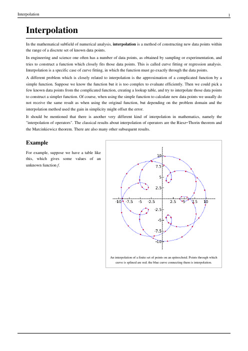
InterpolationIn the mathematical subfield of numerical analysis, interpolation is a method of constructing new data points within the range of a discrete set of known data points.In engineering and science one often has a number of data points, as obtained by sampling or experimentation, and tries to construct a function which closely fits those data points. This is called curve fitting or regression analysis.Interpolation is a specific case of curve fitting, in which the function must go exactly through the data points.A different problem which is closely related to interpolation is the approximation of a complicated function by a simple function. Suppose we know the function but it is too complex to evaluate efficiently. Then we could pick a few known data points from the complicated function, creating a lookup table, and try to interpolate those data points to construct a simpler function. Of course, when using the simple function to calculate new data points we usually do not receive the same result as when using the original function, but depending on the problem domain and the interpolation method used the gain in simplicity might offset the error.It should be mentioned that there is another very different kind of interpolation in mathematics, namely the "interpolation of operators". The classical results about interpolation of operators are the Riesz –Thorin theorem and the Marcinkiewicz theorem. There are also many other subsequent results.An interpolation of a finite set of points on an epitrochoid. Points through whichcurve is splined are red; the blue curve connecting them is interpolation.ExampleFor example, suppose we have a table likethis, which gives some values of anunknown function f .Plot of the data points as given in the table.xf (x )0010.841520.909330.14114−0.75685−0.95896−0.2794Interpolation provides a means of estimating the function at intermediate points, such as x = 2.5.There are many different interpolation methods, some of which are described below. Some of the concerns to take into account when choosing an appropriate algorithm are: How accurate is the method? How expensive is it? How smooth is the interpolant? How many data points are needed?Piecewise constant interpolationPiecewise constant interpolation, ornearest-neighbor interpolation.The simplest interpolation method is to locate the nearest data value,and assign the same value. In one dimension, there are seldom goodreasons to choose this one over linear interpolation, which is almost ascheap, but in higher dimensional multivariate interpolation, this can bea favourable choice for its speed and simplicity.Linear interpolationPlot of the data with linear interpolation superimposedOne of the simplest methods is linear interpolation(sometimes known as lerp). Consider the above example ofdetermining f (2.5). Since 2.5 is midway between 2 and 3, itis reasonable to take f (2.5) midway between f (2) = 0.9093and f (3) = 0.1411, which yields 0.5252.Generally, linear interpolation takes two data points, say(x a ,y a ) and (x b ,y b ), and the interpolant is given by:at the point (x ,y )Linear interpolation is quick and easy, but it is not very precise. Another disadvantage is that the interpolant is not differentiable at the point x k .The following error estimate shows that linear interpolation is not very precise. Denote the function which we want to interpolate by g , and suppose that x lies between x a and x b and that g is twice continuously differentiable. Then the linear interpolation error isIn words, the error is proportional to the square of the distance between the data points. The error of some other methods, including polynomial interpolation and spline interpolation (described below), is proportional to higher powers of the distance between the data points. These methods also produce smoother interpolants.Polynomial interpolationPlot of the data with polynomial interpolation appliedPolynomial interpolation is a generalization of linearinterpolation. Note that the linear interpolant is a linearfunction. We now replace this interpolant by a polynomialof higher degree.Consider again the problem given above. The followingsixth degree polynomial goes through all the seven points:Substituting x = 2.5, we find that f (2.5) = 0.5965.Generally, if we have n data points, there is exactly onepolynomial of degree at most n −1 going through all the datapoints. The interpolation error is proportional to the distancebetween the data points to the power n . Furthermore, theinterpolant is a polynomial and thus infinitely differentiable.So, we see that polynomial interpolation solves all theproblems of linear interpolation.However, polynomial interpolation also has some disadvantages. Calculating the interpolating polynomial is computationally expensive (see computational complexity) compared to linear interpolation. Furthermore, polynomial interpolation may exhibit oscillatory artifacts, especially at the end points (see Runge's phenomenon).These disadvantages can be avoided by using spline interpolation or restricting attention Chebyshev polynomials.Spline interpolationPlot of the data with spline interpolation applied Remember that linear interpolation uses a linear functionfor each of intervals [x k ,x k+1]. Spline interpolation useslow-degree polynomials in each of the intervals, andchooses the polynomial pieces such that they fit smoothlytogether. The resulting function is called a spline.For instance, the natural cubic spline is piecewise cubic andtwice continuously differentiable. Furthermore, its secondderivative is zero at the end points. The natural cubic splineinterpolating the points in the table above is given byIn this case we get f (2.5) = 0.5972.Like polynomial interpolation, spline interpolation incurs asmaller error than linear interpolation and the interpolant issmoother. However, the interpolant is easier to evaluatethan the high-degree polynomials used in polynomial interpolation. It also does not suffer from Runge's phenomenon.Interpolation via Gaussian processesGaussian process is a powerful non-linear interpolation tool. Many popular interpolation tools are actually equivalent to particular Gaussian processes. Gaussian processes can be used not only for fitting an interpolant that passes exactly through the given data points but also for regression, i.e., for fitting a curve through noisy data. In the geostatistics community Gaussian process regression is also known as Kriging.Other forms of interpolationOther forms of interpolation can be constructed by picking a different class of interpolants. For instance, rational interpolation is interpolation by rational functions, and trigonometric interpolation is interpolation by trigonometric polynomials. Another possibility is to use wavelets.The Whittaker –Shannon interpolation formula can be used if the number of data points is infinite.Multivariate interpolation is the interpolation of functions of more than one variable. Methods include bilinear interpolation and bicubic interpolation in two dimensions, and trilinear interpolation in three dimensions.Sometimes, we know not only the value of the function that we want to interpolate, at some points, but also its derivative. This leads to Hermite interpolation problems.Interpolation in Digital Signal ProcessingIn the domain of digital signal processing, the term interpolation refers to the process of converting a sampled digital signal (such as a sampled audio signal) to a higher sampling rate using various digital filtering techniques (e.g.,convolution with a frequency-limited impulse signal). In this application there is a specific requirement that the harmonic content of the original signal be preserved without creating aliased harmonic content of the original signal above the original Nyquist limit of the signal (i.e., above fs/2 of the original signal sample rate). An early and fairly elementary discussion on this subject can be found in Rabiner and Crochiere's book Multirate Digital Signal Processing .[1]Related conceptsThe term extrapolation is used if we want to find data points outside the range of known data points.In curve fitting problems, the constraint that the interpolant has to go exactly through the data points is relaxed. It is only required to approach the data points as closely as possible (within some other constraints). This requires parameterizing the potential interpolants and having some way of measuring the error. In the simplest case this leads to least squares approximation.Approximation theory studies how to find the best approximation to a given function by another function from some predetermined class, and how good this approximation is. This clearly yields a bound on how well the interpolant can approximate the unknown function.See also•Simple rational approximationReferences[1]R.E. Crochiere and L.R. Rabiner. (1983). Multirate Digital Signal Processing. Englewood Cliffs, NJ: Prentice-Hall. (http://www.amazon.com/Multirate-Digital-Signal-Processing-Crochiere/dp/0136051626)Article Sources and Contributors6 Article Sources and ContributorsInterpolation Source: /w/index.php?oldid=384878591 Contributors: A.melkumyan, AlbertSM, Alberto da Calvairate, Algebraist, Andonic, Auntof6, BenFrantzDale,Berland, Betacommand, Bobet, Bobo192, CanadianLinuxUser, Ccooke123, Cdc, Chadernook, ChangChienFu, Chaos, Charles Matthews, Coneslayer, Conversion script, Cronholm144,DavidCary, Dcljr, DerHexer, Dick Beldin, Dicklyon, Dino, DoctorW, Dudzcom, Dungodung, Edrowland, El C, El-Ahrairah, Elwikipedista, Eric119, Everyking, Fgnievinski, Friginator, Giftlite, Grajales, Grunt, HGB, Harp, Hattrem, Hede2000, HenkvD, Herbee, Heron, Hippopottoman, Hyacinth, Ironholds, JJL, JahJah, Jaimeastorga2000, Japo, Jeltz, Jezhotwells, Jitse Niesen,JohnBlackburne, Kieff, Lotje, Marcello Quintieri, Martin.Budden, Math Champion, MathFacts, MathMartin, Matt37, Michael Hardy, Mike Peel, MuzikJunky, Niffux, Oleg Alexandrov, Oli Filth, Omicronpersei8, PabloCastellano, Patrick, Pdcook, Persian Poet Gal, RMFan1, Rich Farmbrough, Roger pearse, SWAdair, Shreevatsa, Spooky, Supertouch, Sławomir Biały, UFu, Uberjivy,Vtstarin, Wi-king, Woodinville, XJamRastafire, Xiaojeng, Yas, 134 anonymous editsImage Sources, Licenses and ContributorsImage:Splined epitrochoid.png Source: /w/index.php?title=File:Splined_epitrochoid.png License: Public Domain Contributors: User:DinoImage:Interpolation Data.svg Source: /w/index.php?title=File:Interpolation_Data.svg License: Public Domain Contributors: User:BerlandImage:Piecewise constant.svg Source: /w/index.php?title=File:Piecewise_constant.svg License: Public Domain Contributors: User:BerlandImage:Interpolation example linear.svg Source: /w/index.php?title=File:Interpolation_example_linear.svg License: Public Domain Contributors: User:BerlandImage:Interpolation example polynomial.svg Source: /w/index.php?title=File:Interpolation_example_polynomial.svg License: Public Domain Contributors:User:BerlandImage:Interpolation example spline.svg Source: /w/index.php?title=File:Interpolation_example_spline.svg License: Public Domain Contributors: User:Berland LicenseCreative Commons Attribution-Share Alike 3.0 Unported/licenses/by-sa/3.0/。
Combinatorial Nullstellensatz
h i gi .
s∈Si (xi
In the special case m = n, where each gi is a univariate polynomial of the form stronger conclusion holds, as follows.
− s), a
Theorem 1.1 Let F be an arbitrary field, and let f = f (x1 , . . . , xn ) be a polynomial in F [x1 , . . . , xn ]. Let S1 , . . . , Sn be nonempty subsets of F and define gi2 , . . . , sn ∈ Sn so that
In this paper we prove these two theorems, which may be called Combinatorial Nullstellensatz, and describe several combinatorial applications of them. After presenting the (simple) proofs of the above theorems in Section 2, we show, in Section 3 that the classical theorem of Chevalley and Warning on roots of systems of polynomials as well as the basic theorem of Cauchy and Davenport on the addition of residue classes follow as simple consequences. We proceed to describe additional applications in Additive Number Theory and in Graph Theory and Combinatorics in Sections 4,5,6,7 and 8. Many of these applications are known results, proved here in a unified way, and some are new. There are several known results that assert that a combinatorial structure satisfies certain combinatorial property if and only if an appropriate polynomial associated with it lies in a properly defined ideal. In Section 9 we apply our technique and obtain several new results of this form. The final Section 10 contains some concluding remarks and open problems.
数值分析(英语版)常见英语翻译
absolute error绝对误差,relative error and significant digits 相对误差和有效数字(n-digit)accurate to 5 decimal places精确到5位小数degree accuracy准确度Newton-Raphson formula牛顿-拉夫森公式Root根sum of和Newton-cotes牛顿—柯特斯Coefficients系数Convergence集合sufficient and necessary condition充分必要条件iterative formula迭代公式fixed point bisection method固定点的二分法fixed point iteration固定点迭代法integration积分法linear system线性方程组triangular factorization三角分解Gauss-Seidel iteration高斯-赛德尔迭代Gaussian elimination高斯消去法,高斯消元;Jacobi method雅可比法the clamped cubic spline夹紧的三次样条the first derivative一阶导数curve fitting曲线拟合the least-squares line coefficient最小二乘线系数function函数Polynomial多项式node结点of degree n度degree of precision精密度interpolation插值approximate逼近,近似error term误差项tend to倾向于cubic spline Taylor interpolation三次样条函数的泰勒插值Hermite interpolation埃尔米特插值high-degree polynomials高阶多项式quadrature formula求积分公式constant Simpson’s rule常数辛普森规则Trapezoidal’s rule composite Simpson rule 组合梯形公式和辛普森公式Integral积分the initial value problem初始值问题Euler’s method欧拉方法spectral radius谱半径norm interval规范区间Chebyshev polynomial切比雪夫多项式strengths and weaknesses长处和短处definite integral定积分quadratic Lagrange interpolation二次拉格朗日插值divided-difference table 差分表compute计算三角分解插值切比雪夫三次样条代数精度Gauss_Seidel, Jocabi, Euler,插值型求积公式。
derivate_gauss计算过程

derivate_gauss计算过程Gauss's method of derivative computation, also known as Gauss's derivative formula or Gauss's differentiation formula, is a mathematical technique for finding the derivative of a function using polynomial interpolation.The general formula for the derivative of a function f(x) at a point x0 is given by:f'(x0) = ( f(x1) * w1 + f(x2) * w2 + ... + f(xn) * wn ) / hwhere x1, x2, ..., xn are equally spaced points around x0, h is the distance between the points, and w1, w2, ..., wn are the weights assigned to each point.The weights can be determined using polynomial interpolation. To do this, we first need to construct a polynomial of degree n-1 that passes through the points (x1, f(x1)), (x2, f(x2)), ..., (xn, f(xn)). This polynomial can be written as:P(x) = f(x1) * L1(x) + f(x2) * L2(x) + ... + f(xn) * Ln(x)where L1(x), L2(x), ..., Ln(x) are the Lagrange basis polynomials defined as:Li(x) = (x - x1) * (x - x2) * ... * (x - xi-1) * (x - xi+1) * ... * (x - xn) / (xi - x1) * (xi - x2) * ... * (xi - xi-1) * (xi - xi+1) * ... * (xi - xn) Next, we differentiate the polynomial P(x) with respect to x and evaluate it at x0:f'(x0) = P'(x0) = f(x1) * L1'(x0) + f(x2) * L2'(x0) + ... + f(xn) *Ln'(x0)The derivative of the Lagrange basis polynomials can be calculated as:Li'(x) = [(x - x1) * (x - x2) * ... * (x - xi-1) * (x - xi+1) * ... * (x - xn)]' / [(xi - x1) * (xi - x2) * ... * (xi - xi-1) * (xi - xi+1) * ... * (xi - xn)]To simplify the derivative expression, we can expand the numerator and denominator using the product rule and then cancel out common terms:Li'(x) = [x - x1 + x - x2 + ... + x - xi-1 + x - xi+1 + ... + x - xn] / [(xi - x1) * (xi - x2) * ... * (xi - xi-1) * (xi - xi+1) * ... * (xi - xn)] Simplifying further, we have:Li'(x) = [(n-1)x - (x1 + x2 + ... + xi-1 + xi+1 + ... + xn)] / [(xi - x1) * (xi - x2) * ... * (xi - xi-1) * (xi - xi+1) * ... * (xi - xn)]Finally, we evaluate Li'(x) at x0 to get the weights wi:wi = [(n-1)x0 - (x1 + x2 + ... + xi-1 + xi+1 + ... + xn)] / [(xi - x1) * (xi - x2) * ... * (xi - xi-1) * (xi - xi+1) * ... * (xi - xn)]By substituting these weights and the function values f(x1),f(x2), ..., f(xn) into the derivative formula, we can compute thederivative f'(x0) using Gauss's method.It is important to note that Gauss's method of derivative computation assumes that the function f(x) is well-behaved and can be approximated by a polynomial in the neighborhood of x0. This technique works best when the points x1, x2, ..., xn are equally spaced and close to x0.(Source: Introduction to Numerical Analysis by J. Stoer and R. Bulirsch)。
2013年美国AIME数学邀请赛I,II
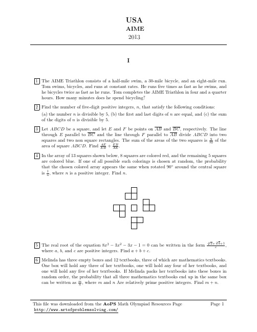
2013I 1The AIME Triathlon consists of a half-mile swim,a 30-mile bicycle,and an eight-mile run.Tom swims,bicycles,and runs at constant rates.He runs five times as fast as he swims,and he bicycles twice as fast as he runs.Tom completes the AIME Triathlon in four and a quarter hours.How many minutes does he spend bicycling?2Find the number of five-digit positive integers,n ,that satisfy the following conditions:(a)the number n is divisible by 5,(b)the first and last digits of n are equal,and (c)the sum of the digits of n is divisible by 5.3Let ABCD be a square,and let E and F be points on AB and BC ,respectively.The line through E parallel to BC and the line through F parallel to AB divide ABCD into twosquares and two non square rectangles.The sum of the areas of the two squares is 910of thearea of square ABCD .Find AE EB +EB AE .4In the array of 13squares shown below,8squares are colored red,and the remaining 5squares are colored blue.If one of all possible such colorings is chosen at random,the probability that the chosen colored array appears the same when rotated 90◦around the central square is 1n ,where n is a positive integer.Find n .5The real root of the equation 8x 3−3x 2−3x −1=0can be written in the form3√a +3√b +1c,where a ,b ,and c are positive integers.Find a +b +c .6Melinda has three empty boxes and 12textbooks,three of which are mathematics textbooks.One box will hold any three of her textbooks,one will hold any four of her textbooks,and one will hold any five of her textbooks.If Melinda packs her textbooks into these boxes in random order,the probability that all three mathematics textbooks end up in the same box can be written as m n ,where m and n Are relatively prime positive integers.Find m +n .This file was downloaded from the AoPS Math Olympiad Resources PagePage 120137A rectangular box has width 12inches,length 16inches,and height m n inches,where m and n are relatively prime positive integers.Three faces of the box meet at a corner of the box.The center points of those three faces are the vertices of a triangle with an area of 30square inches.Find m +n .8The domain of the function f (x )=arcsin(log m (nx ))is a closed interval of length 12013,wherem and n are positive integers and m >1.Find the remainder when the smallest possible sum m +n is divided by 1000.9A paper equilateral triangle ABC has side length 12.The paper triangle is folded so that vertex A touches a point on side BC a distance 9from point B .The length of the line segment along which the triangle is folded can be written as m √p n ,where m ,n ,and p are positive integers,m and n are relatively prime,and p is not divisible by the square of any prime.Find m +n +p.B CB AC 10There are nonzero integers a ,b ,r ,and s such that the complex number r +si is a zero of thepolynomial P (x )=x 3−ax 2+bx −65.For each possible combination of a and b ,let p a,b be the sum of the zeroes of P (x ).Find the sum of the p a,b ’s for all possible combinations of a and b .11Ms.Math’s kindergarten class has 16registered students.The classroom has a very largenumber,N ,of play blocks which satisfies the conditions:(a)If 16,15,or 14students are present,then in each case all the blocks can be distributed in equal numbers to each student,and (b)There are three integers 0<x <y <z <14such that when x ,y ,or z students are present and the blocks are distributed in equal numbers to each student,there are exactly three blocks left over.Find the sum of the distinct prime divisors of the least possible value of N satisfying the above conditions.201312Let P QR be a triangle with ∠P =75◦and ∠Q =60◦.A regular hexagon ABCDEF withside length 1is drawn inside P QR so that side AB lies on P Q ,side CD lies on QR ,andone of the remaining vertices lies on RP .There are positive integers a ,b ,c ,and d such that the area of P QR can be expressed in the form a +b √cd ,where a and d are relatively primeand c is not divisible by the square of any prime.Find a +b +c +d .13Triangle AB 0C 0has side lengths AB 0=12,B 0C 0=17,and C 0A =25.For each positiveinteger n ,points B n and C n are located on AB n −1and AC n −1,respectively,creating three similar triangles AB n C n ∼ B n −1C n C n −1∼ AB n −1C n −1.The area of the union of all triangles B n −1C n B n for n ≥1can be expressed as pq ,where p and q are relatively primepositive integers.Find q .14For π≤θ<2π,letP =12cos θ−14sin 2θ−18cos 3θ+116sin 4θ+132cos 5θ−164sin 6θ−1128cos 7θ+...and Q =1−12sin θ−14cos 2θ+18sin 3θ+116cos 4θ−132sin 5θ−164cos 6θ+1128sin 7θ+...so that P Q =2√27.Then sin θ=−m n where m and n are relatively prime positive integers.Find m +n .15Let N be the number of ordered triples (A,B,C )of integers satisfying the conditions(a)0≤A <B <C ≤99,(b)there exist integers a ,b ,and c ,and prime p where 0≤b <a <c <p ,(c)p divides A −a ,B −b ,and C −c ,and (d)each ordered triple (A,B,C )and each ordered triple (b,a,c )form arithmetic sequences.Find N .2013II 1Suppose that the measurement of time during the day is converted to the metric system so that each day has 10metric hours,and each metric hour has 100metric minutes.Digital clocks would then be produced that would read 9:99just before midnight,0:00at midnight,1:25at the former 3:00am ,and 7:50at the former 6:00pm .After the conversion,a person who wanted to wake up at the equivalent of the former 6:36am would have to set his new digital alarm clock for A:BC,where A,B,and C are digits.Find 100A +10B +C.2Positive integers a and b satisfy the conditionlog 2(log 2a (log 2b (21000)))=0.Find the sum of all possible values of a +b .3A large candle is 119centimeters tall.It is designed to burn down more quickly when it is first lit and more slowly as it approaches its bottom.Specifically,the candle takes 10seconds to burn down the first centimeter from the top,20seconds to burn down the second centimeter,and 10k seconds to burn down the k -th centimeter.Suppose it takes T seconds for the candle to burn down completely.Then T 2seconds after it is lit,the candle’s height in centimeters will be h .Find 10h .4In the Cartesian plane let A =(1,0)and B = 2,2√3 .Equilateral triangle ABC is con-structed so that C lies in the first quadrant.Let P =(x,y )be the center of ABC .Then x ·y can be written as p √q r ,where p and r are relatively prime positive integers and q is an integer that is not divisible by the square of any prime.Find p +q +r .5In equilateral ABC let points D and E trisect BC .Then sin (∠DAE )can be expressed in the form a √b c ,where a and c are relatively prime positive integers,and b is an integer that is not divisible by the square of any prime.Find a +b +c .6Find the least positive integer N such that the set of 1000consecutive integers beginning with 1000·N contains no square of an integer.7A group of clerks is assigned the task of sorting 1775files.Each clerk sorts at a constant rate of 30files per hour.At the end of the first hour,some of the clerks are reassigned to another task;at the end of the second hour,the same number of the remaining clerks are also reassigned to another task,and a similar reassignment occurs at the end of the third hour.The group finishes the sorting in 3hours and 10minutes.Find the number of files sorted during the first one and a half hours of sorting.20138A hexagon that is inscribed in a circle has side lengths 22,22,20,22,22,and 20in that order.The radius of the circle can be written as p +√q ,where p and q are positive integers.Find p +q .9A 7×1board is completely covered by m ×1tiles without overlap;each tile may cover any number of consecutive squares,and each tile lies completely on the board.Each tile is either red,blue,or green.Let N be the number of tilings of the 7×1board in which all three colors are used at least once.For example,a 1×1red tile followed by a 2×1green tile,a 1×1green tile,a 2×1blue tile,and a 1×1green tile is a valid tiling.Note that if the 2×1blue tile is replaced by two 1×1blue tiles,this results in a different tiling.Find the remainder when N is divided by 1000.10Given a circle of radius √13,let A be a point at a distance 4+√13from the center O of thecircle.Let B be the point on the circle nearest to point A .A line passing through the point A intersects the circle at points K and L .The maximum possible area for BKL can bewritten in the form a −b √c d ,where a ,b ,c ,and d are positive integers,a and d are relativelyprime,and c is not divisible by the square of any prime.Find a +b +c +d .11Let A ={1,2,3,4,5,6,7}and let N be the number of functions f from set A to set A suchthat f (f (x ))is a constant function.Find the remainder when N is divided by 1000.12Let S be the set of all polynomials of the form z 3+az 2+bz +c ,where a ,b ,and c are integers.Find the number of polynomials in S such that each of its roots z satisfies either |z |=20or |z |=13.13In ABC ,AC =BC ,and point D is on BC so that CD =3·BD .Let E be the midpoint of AD .Given that CE =√7and BE =3,the area of ABC can be expressed in the form m √n ,where m and n are positive integers and n is not divisible by the square of any prime.Find m +n .14For positive integers n and k ,let f (n,k )be the remainder when n is divided by k ,and forn >1let F (n )=max 1≤k ≤n 2f (n,k ).Find the remainder when 100 n =20F (n )is divided by 1000.15Let A,B,C be angles of an acute triangle withcos 2A +cos 2B +2sin A sin B cos C =158and cos 2B +cos 2C +2sin B sin C cos A =149.There are positive integers p ,q ,r ,and s for which cos 2C +cos 2A +2sin C sin A cos B =p −q √r s ,2013where p+q and s are relatively prime and r is not divisible by the square of any prime.Find p+q+r+s.。
Legendre Polynomial
Legendre PolynomialThe Legendre polynomials, sometimes called Legendre functions of the first kind, Legendre coefficients, or zonal harmonics(Whittaker and Watson 1990, p. 302), are solutions to the Legendre differential equation. If is an integer, they are polynomials. The Legendre polynomials are illustrated above for and , 2, ..., 5. They are implemented in Mathematica as LegendreP[n, x].The Legendre polynomial can be defined by the contour integral(1)where the contour encloses the origin and is traversed in a counterclockwise direction (Arfken 1985, p. 416).The first few Legendre polynomials are(2)(3)(4)(5)(6)(7)(8)When ordered from smallest to largest powers and with the denominators factored out, the triangle of nonzero coefficients is 1, 1, , 3, , 5, 3, , ... (Sloane's A008316). The leading denominators are 1, 1, 2, 2, 8, 8, 16, 16, 128, 128, 256, 256, ... (Sloane's A060818).The first few powers in terms of Legendre polynomials are(9)(10)(11)(12)(13)(14) (Sloane's A008317 and A001790). A closed form for these is given by(15)(R. Schmied, pers. comm., Feb. 27, 2005). For Legendre polynomials and powers up to exponent 12, see Abramowitz and Stegun (1972, p. 798).The Legendre polynomials can also be generated using Gram-Schmidt orthonormalization in the open interval with the weighting function 1.(16)(17)(18)(19)(20)(21)(22)Normalizing so that gives the expected Legendre polynomials.The "shifted" Legendre polynomials are a set of functions analogous to the Legendre polynomials, but defined on the interval (0, 1). They obey the orthogonality relationship(23)The first few are(24)(25)(26)(27) The Legendre polynomials are orthogonal over with weighting function 1 and satisfy(28)where is the Kronecker delta.The Legendre polynomials are a special case of the ultraspherical functions with , a special case of theJacobi polynomials with , and can be written as a hypergeometric function using Murphy's formula(29)(Bailey 1933; 1935, p. 101; Koekoek and Swarttouw 1998).The Rodrigues representation provides the formula(30) which yields upon expansion(31)(32) where is the floor function. Additional sum formulas include(33)(34) (Koepf 1998, p. 1). In terms of hypergeometric functions, these can be written(35)(36)(37) (Koepf 1998, p. 3).A generating function for is given by(38) Take ,(39) Multiply (39) by ,(40) and add (38) and (40),(41)This expansion is useful in some physical problems, including expanding the Heyney-Greenstein phase function and computing the charge distribution on a sphere. Another generating function is given by(42)where is a zeroth order Bessel function of the first kind (Koepf 1998, p. 2).The Legendre polynomials satisfy the recurrence relation(43) (Koepf 1998, p. 2). In addition,(44)(correcting Hildebrand 1956, p. 324).A complex generating function is(45) and the Schläfli integral is(46) Integrals over the interval include the general formula(47) for (Byerly 1959, p. 172), from which the special case(48)(49)follows (Sloane's A002596and A046161; Byerly 1959, p. 172). For the integral over a product of Legendre functions,(50)for (Byerly 1959, p. 172), which gives the special case(51) where(52)(Sloane's A078297 and A078298; Byerly 1959, p. 172). The latter is a special case of(53) where(54)and is a gamma function (Gradshteyn and Ryzhik 2000, p. 762, eqn. 7.113.1)Integrals over with weighting functions and are given by(55)(56)(Arfken 1985, p. 700).The Laplace transform is given by(57)where is a modified Bessel function of the first kind.A sum identity is given by(58) where is the th root of (Szegö 1975, p. 348). A similar identity is(59) which is responsible for the fact that the sum of weights in Legendre-Gauss quadrature is always equal to 2.The associated Legendre polynomials and are solutions to the associated Legendre differentialequation, where is a positive integer and , ..., . They are implemented in Mathematica as LegendreP[l, m, x]. For positive , they can be given in terms of the unassociated polynomials by(60)(61)where are the unassociated Legendre polynomials. The associated Legendre polynomials for negative are then defined by(62)There are two sign conventions for associated Legendre polynomials. Some authors (e.g., Arfken 1985, pp. 668-669) omit the Condon-Shortley phase, while others include it (e.g., Abramowitz and Stegun 1972, Press et al. 1992, and the LegendreP[l, m, z] command of Mathematica). Care is therefore needed in comparing polynomials obtained from different sources. One possible way to distinguish the two conventions is due to Abramowitz and Stegun (1972, p. 332), who use the notation(63) to distinguish the two.Associated polynomials are sometimes called Ferrers' functions (Sansone 1991, p. 246). If , they reduce to the unassociated polynomials. The associated Legendre functions are part of the spherical harmonics, which are the solution of Laplace's equation in spherical coordinates. They are orthogonal over with the weighting function 1(64)and orthogonal over with respect to with the weighting function,(65)The associated Legendre polynomials also obey the following recurrence relations(66) Letting (commonly denoted in this context),(67)(68)Additional identities are(69)(70) Including the factor of , the first few associated Legendre polynomials are(71)(72)(73)(74)(75)(76)(77)(78)(79)(80)(81)(82)(83)(84)(85)(86) Written in terms (commonly written ), the first few become(87)(88)(89)(90)(91)(92)(93)(94)(95)(96) The derivative about the origin is(97)(Abramowitz and Stegun 1972, p. 334), and the logarithmic derivative is(98)(Binney and Tremaine 1987, p. 654).SEE ALSO:Condon-Shortley Phase, Conical Function, Kings Problem, Laplace's Integral, Laplace-Mehler Integral, Legendre Function of the First Kind, Legendre Function of the Second Kind, Mehler-Dirichlet Integral, Spherical Harmonic, Super Catalan Number, Toroidal Function, Turán's Inequalities, Ultraspherical Polynomial, Zonal HarmonicRELATED WOLFRAM SITES:/Polynomials/LegendreP/, /Polynomials/LegendreP/REFERENCES:Abramowitz, M. and Stegun, I. A. (Eds.). "Legendre Functions" and "Orthogonal Polynomials." Ch. 22 in Chs. 8 and 22 in Handbook of Mathematical Functions with Formulas, Graphs, and Mathematical Tables, 9th printing. New York: Dover, pp. 331-339 and 771-802, 1972.Arfken, G. "Legendre Functions." Ch. 12 in Mathematical Methods for Physicists, 3rd ed. Orlando, FL: Academic Press, pp. 637-711, 1985.Bailey, W. N. "On the Product of Two Legendre Polynomials." Proc. Cambridge Philos. Soc.29, 173-177, 1933. Bailey, W. N. Generalised Hypergeometric Series. Cambridge, England: Cambridge University Press, 1935. Binney, J. and Tremaine, S. "Associated Legendre Functions." Appendix 5 in Galactic Dynamics.Princeton, NJ: Princeton University Press, pp. 654-655, 1987.Byerly, W. E. "Zonal Harmonics." Ch. 5 in An Elementary Treatise on Fourier's Series, and Spherical, Cylindrical, and Ellipsoidal Harmonics, with Applications to Problems in Mathematical Physics.New York: Dover, pp. 144-194, 1959.Gradshteyn, I. S. and Ryzhik, I. M. Tables of Integrals, Series, and Products, 6th ed. San Diego, CA: Academic Press, 2000.Hildebrand, F. B. Introduction to Numerical Analysis. New York: McGraw-Hill, 1956.Iyanaga, S. and Kawada, Y. (Eds.). "Legendre Function" and "Associated Legendre Function." Appendix A, Tables 18.II and 18.III in Encyclopedic Dictionary of Mathematics. Cambridge, MA: MIT Press, pp. 1462-1468, 1980. Koekoek, R. and Swarttouw, R. F. "Legendre / Spherical." §1.8.3 in The Askey-Scheme of HypergeometricOrthogonal Polynomials and its -Analogue. Delft, Netherlands: Technische Universiteit Delft, Faculty of Technical Mathematics and Informatics Report 98-17, p. 44, 1998.Koepf, W. Hypergeometric Summation: An Algorithmic Approach to Summation and Special Function Identities. Braunschweig, Germany: Vieweg, 1998.Lagrange, R. Polynomes et fonctions de Legendre. Paris: Gauthier-Villars, 1939.Legendre, A. M. "Sur l'attraction des Sphéroides." Mém. Math. et Phys. présentés à l'Ac. r. des. sc. par divers savants10, 1785.Morse, P. M. and Feshbach, H. Methods of Theoretical Physics, Part I. New York: McGraw-Hill, pp. 593-597, 1953. Press, W. H.; Flannery, B. P.; Teukolsky, S. A.; and Vetterling, W. T. Numerical Recipes in FORTRAN: The Art of Scientific Computing, 2nd ed. Cambridge, England: Cambridge University Press, p. 252, 1992.Sansone, G. "Expansions in Series of Legendre Polynomials and Spherical Harmonics." Ch. 3 in Orthogonal Functions, rev. English ed. New York: Dover, pp. 169-294, 1991.Sloane, N. J. A. Sequences A001790/M2508, A002596/M3768, A008316, A008317, A046161, A060818, A078297, and A078298 in "The On-Line Encyclopedia of Integer Sequences."Snow, C. Hypergeometric and Legendre Functions with Applications to Integral Equations of Potential Theory. Washington, DC: U. S. Government Printing Office, 1952.Spanier, J. and Oldham, K. B. "The Legendre Polynomials " and "The Legendre Functions and ." Chs. 21 and 59 in An Atlas of Functions. Washington, DC: Hemisphere, pp. 183-192 and 581-597, 1987.Strutt, J. W. "On the Values of the Integral , , being LaPlace's Coefficients of the orders ,, with an Application to the Theory of Radiation." Philos. Trans. Roy. Soc. London160, 579-590, 1870.Szegö, G. Orthogonal Polynomials, 4th ed. Providence, RI: Amer. Math. Soc., 1975.Whittaker, E. T. and Watson, G. N. A Course in Modern Analysis, 4th ed. Cambridge, England: Cambridge University Press, 1990.。
1 WHAT IS O-MINIMALITY
WHAT IS O-MINIMALITY?byHarvey M. Friedman*Ohio State Universityfriedman@/%7Efriedman/November 8, 2006Revised September 6, 2007Revised October 29, 2007Revised November 30, 2007Abstract. We characterize the o-minimal expansions of thering of real numbers, in mathematically transparent terms.This should help bridge the gap between investigators in o-minimality and mathematicians unfamiliar with model theory,who are concerned with such notions as non oscillatorybehavior, tame topology, and analyzable functions. We adapt the characterization to the case of o-minimal expansions of an arbitrary ordered ring.1. PRELIMINARIES.We give a new characterization of o-minimal expansions of the ring of real numbers, in particularly transparent mathematical terms. The reader may wish to compare the characterization here with the approach of [Dr98], p.13, which can be adapted to give a characterization in terms of relations instead of functions.The main definition is that of a rich class (¬). The (¬) indicates that we are working over the ring of real numbers.We say that V is a rich class (¬) if and only if1. MULTIVARIATE (¬). All elements of V are functions f such that the domain of f is some ¬n and the range of f is a subset of some ¬m.2. POLYNOMIALS (¬). Every polynomial with real coefficients from any ¬n into any ¬m is an element of V.3. COMPOSITION (¬).i. If f:¬nƬmŒ V, g:¬mƬpŒ V, then h:¬nƬpŒ V, where for all x Œ¬n, h(x) = g(f(x)).ii. If f:¬nƬmŒ V, g:¬nƬpŒ V, then h:¬nƬm+pŒ V, where for all x Œ¬n, h(x) = (f(x),g(x)).4. ZERO SELECTION (¬). Let f:¬n+mƬŒ V. There existsg:¬nƬmŒ V such that if f(x,y) = 0 then f(x,g(x)) = 0.We use the adjective “special” if, in addition, we have5. LIMIT (¬). Every bounded f:¬Æ¬Œ V has a limit at infinity.From model theory, an expansion of the ring of real numbers is a system (¬,<,0,1,+,-,•,V), where V obeys MULTIVARIATE (¬).From model theory, an o-minimal expansion of the ring ofreal numbers is an expansion of the ring of real numbers in which every first order definable subset of ¬ is a finite union of open intervals and points. Here • and -• are allowed as endpoints. Here, and throughout the paper, "definable" means "definable with parameters by a formulain the first order predicate calculus with equality".The above definition is a special case of the more general definition of o-minimal structure introduced in [PS86], which we use in section 4.Specifically, a linearly ordered structure is a system(D,<,V), where (D,<) is a strictly linear ordering, and Vis a set of constants from D, multivariate relations on D, and multivariate functions from D into D. An o-minimal structure is a structure M = (D,<,V), where every Mdefinable subset of D is a finite union of open intervals and points, where the endpoints of the intervals lie in D »{-•,•} and the points lie in D.We prove the following.THEOREM A. Let M = (¬,<,0,1,+,-,•,V) be an expansion of the ring of real numbers. The following are equivalent.i. M is o-minimal.ii. V is a subset of some special rich class (¬).ii. There is a least rich class (¬) containing V, and this rich class (¬) is special.We conclude with Theorem B, which is a version forarbitrary ordered rings.2. RICH CLASSES OF REAL FUNCTIONS.The key to proving Theorem A is the characterization ofrich classes (¬) in terms of first order definability. We now fix V to be a rich class (¬). Let M = (¬,<,0,1,+,-,•,V).Let f:¬n+mƬ. A zero selector of f is a g with the property in the ZERO SELECTION (¬) clause.LEMMA 2.1. There exist f1,...,f8:¬Æ¬Œ V and f9,...,f12:¬4Ƭ such thati. f1(x) = 1/x if x ≠ 0.ii. f2(x) = 0 if x ≠ 0; 1 otherwise.iii. f3(0) = 0; f3(x) = 1 elsewhere.iv. x ≥ 0 ´ (f4(x) = sqrt(x) ⁄ f4(x) = -sqrt(x)).v. f5(x) = 0 ´ x ≥ 0.vi. f6(x) = 0 ´ x > 0.vii. f7(x) = 0 if x ≥ 0; 1 otherwise.viii. f8(x) = 0 if x > 0; 1 otherwise.ix. f9(x,y,z,w) = z if x £ y; w otherwise.x. f10(x,y,z,w) = z if x < y; w otherwise.xi. f11(x,y,z,w) = z if x ≠ y; w otherwise.xii. f12(x,y,z,w) = z if x = y; w otherwise.Proof: i. Let f(x,y) = xy-1. Let f1 be a zero selector of f. ii. Let f2(x) = 1-xf1(x).iii. Let f3(x) = 1-f2(x).iv. Let f(x,y) = y2-x. Let f4 be a zero selector for f.v. Let f5(x) = f4(x)2-x.vi. Let f6(x) = f5(x)2 + f2(x)2.vii. f7(x) = f3(f5(x)).viii. Let f8(x) = f3(f6(x)).ix. Let f9(x,y,z,w) = z(1-f7(y-x)) + w(f7(y-x)).x. Let f10(x,y,z,w) = z(1-f8(y-x)) + w(f8(y-x)).xi. Let f11(x,y,z,w) = z(f3(x-y)) + w(1-f3(x-y)).xii. Let f12(x,y,z,w) = z(1-f3(x-y)) + w(f3(x-y)).QEDLet t be a term in the language of M = (¬,<,0,1,+,-,•,V), whose variables are among v1,...,v n, n ≥ 0. I.e., t is an expression built up from 0,1,+,-,•, the functions in V, andthe variables v1,...,v n, in the standard way. For x1,...,x nŒ¬, We write Val(M,t;x1,...,x n) for the value of t in M, when we interpret the variables v1,...,v n as the real numbersx1,...,x n.Let j be a first order formula in the language of M whose free variables are among v1,...,v n, n ≥ 0. We writeSat(M,j;x1,...,x n) to indicate that the formula j is true in M, when we interpret v1,...,v n as the real numbers x1,...,x n.LEMMA 2.2. Let t be a term in the language of M, whose variables are among v1,...,v n, n ≥ 1. Then the function from ¬n into ¬ given by Val(M,t;x1,...,x n) lies in V.Proof: Fix n ≥ 1. We prove by induction on terms with variables among x1,...,x n, that Val(M,t;x1,...,x n) lies in V.case 1. t is x i or a constant. Note that Val(M,t;x1,...,x n)is a polynomial.case 2. t is f(s1,...,s k), where f Œ V. By the induction hypothesis, each function Val(M,s i;x1,...,x n) lies in V. Hence the function(Val(M,s1;x1,...,x n),..., Val(M,s k;x1,...,x n))lies in V. Hence the functionf(Val(M,s1;x1,...,x n),..., Val(M,s k;x1,...,x n)) =Val(M,t;x1,...,x n)lies in V. QEDLEMMA 2.3. Let j be a first order formula in the languageof M whose free variables are among v1,...,v n, n ≥ 1. Then the function f(x1,...,x n) = 1 if Sat(M,j;x1,...,x n); 0 otherwise, lies in V.Proof: We prove the following by induction on j. For all n ≥1 and formulas j whose free variables are among x1,...,x n, the function f(x1,...,x n) = 1 if Sat(M,j;x1,...,x n); 0 otherwise, lies in V.case 1. s = t. Let the (free) variables in s = t be amongv1,...,v n. By Lemma 2.2, the functionsVal(M,s;x1,...,x n)Val(M,t;x1,...,x n)lie in V. The function in question isf(x1,...,x n) = 1 if Val(M,s;x1,...,x n) = Val(M,t;x1,...,x n);0 otherwise.We can rewrite f asf(x1,...,x n) =f12(Val(M,s;x1,...,x n),Val(M,t;x1,...,x n),1,0)and apply Lemmas 2.1, 2.2.case 2. s < t. Let the (free) variables in s = t be amongv1,...,v n. By Lemma 2.2, the functionsVal(M,s;x1,...,x n)Val(M,t;x1,...,x n)lie in V. The function in question isf(x1,...,x n) = 1 if Val(M,s;x1,...,x n) < Val(M;t;x1,...,x n);0 otherwise.We can rewrite f asf(x1,...,x n) =f10(Val(M,s;x1,...,x n),Val(M,t;x1,...,x n),1,0)and apply Lemmas 2.1, 2.2.case 3. ÿj. Let the free variables in ÿj be among v1,...,v n. Then the free variables in ÿj are among v1,...,v n. Let n-ary f be given by the induction hypothesis. The function in question is1-f(x1,...,x n)which lies in V by Lemma 2.2.case 4. jŸy. Let the free variables in jŸy be amongv1,...,v n. Then the free variables in j,y are amongv1,...,v n. Let n-ary f,g be given by the inductionhypothesis for j,y, respectively. The function in question isf(x1,...,x n)•g(x1,...,x n)which lies in V by Lemma 2.2.case 5. ($v p)(j). Let the free variables in ($v p)(j) be among v1,...,v n, where p £ n. (The case p > n will be handled later). Then the free variables in j are amongv1,...,v n. By the induction hypothesis, the functionf(x1,...,x n) = 1 if Sat(M,j;x1,...,x n);0 otherwiselies in V. Defineg(x1,...,x n,y) = 0 if f(x1,...,x p-1,y,x p+1,...,x n) = 1;1 otherwise.By Lemma 2.2, g Œ V. Let h:¬nƬ be a zero selector for g. Finally, let f*:¬nƬ be given byf*(x1,...,x n) = 1 iff(x1,...,x p-1,,h(x1,...,x n),x p+1,...,x n) = 1;0 otherwise.Then f* Œ V and f* is as required.Now suppose p > n. Then the free variables in ($v p)(j) are among v1,...,v p. The argument given above can be repeated with n replaced by p to show that the functionh(x1,...,x p) = 1 if Sat(M,($v p)(j);x1,...,x p);0 otherwiselies in V. The function in question,f(x1,...,x n) = 1 if Sat(M,($x p)(j);x1,...,x n)can be written in the formf(x1,...,x n) = h(x1,...,x n,x n,...,x n)and so by Lemma 2.2, is also in V.The remaining cases ", ⁄, Æ, ´, are left to the reader. QEDLEMMA 2.4. Let f:¬nƬm be first order definable in M. Then f Œ V.Proof: Let f be as given. By Lemma 2.3, the functiong(x1,...,x n+m) = 1 if f(x1,...,x n) ≠ (x n+1,...,x n+m);0 otherwiselies in V. Let h:¬nƬmŒ V be a zero selector for g. Then h = f Œ V. QEDTHEOREM 2.5. Let V obey MULTIVARIATE (¬), and M =(¬,<,0,1,+,-,•,V). The following are equivalent.i. V is a rich class (¬).ii. Every function f:¬n+mƬ definable in M has a zero selector in V.iii. Every function f:¬nƬm definable in M is an element of V, and every function f:¬n+mƬ definable in M has a zero selector in V.Proof: Let V,M be as given. We show i Æ ii Æ iii Æ i.Assume i. Let V be a rich class (¬). Let f:¬n+mƬ be definable in M. By Lemma 2.4, f Œ V. By ZERO SELECTION (¬), f has a zero selector in V.Assume ii. Let f:¬nƬm be definable in M. Let g:¬n+mƬbe defined by g(x,y) = 0 if y = f(x); 1 otherwise. Then gis definable in M. Let h:¬nƬmŒ V be a zero selector for g. Then h = f, and so f Œ V.Assume iii. Since all polynomials are definable in M, and the composition of functions definable in M is definable in M, we have POLYNOMIAL (¬) and COMPOSITION (¬). Also ZERO SELECTION (¬) is immediate. Hence i. QED3. PROOF OF THEOREM A.Recall the definition of a special rich class (¬):V is a special rich class (¬) if and only if V is a rich class (¬) obeying LIMIT (¬).In the proof of Theorem A, we shall use the followingcrucial fact about o-minimal expansions of the ring of real numbers.MONOTONICITY THEOREM. Let M = (¬,<,0,1,+,-,•,V) be an o-minimal expansion of the ring of real numbers. For all f:¬Æ¬Œ V, there exists x1 < ... < x k, k ≥ 1, such that oneach of the complementary open intervals (-•,x1),(x1,x2),...,(x k-1,x k),(x k,•), f is continuous, and f is either constant, strictly increasing, or strictly decreasing. In fact, this is true for any o-minimalstructure M = (D,<,V).This result was first proved in [PS86]. In fact, it was proved there for general o-minimal structures. It is fundamental to the entire theory of o-minimality. Also see [Dr98], p.3, 43-46. In the notation there, x i is allowed to be • or -•.We will not be using the continuity from the Monotonicity Theorem.THEOREM A. Let M = (¬,<,0,1,+,-,•,W) be an expansion of the ring of real numbers. The following are equivalent.i. M is o-minimal.ii. W is a subset of some special rich class (¬).iii. There is a least rich class (¬) containing W, and this rich class (¬) is special.Proof: Let M be as given. We shall prove ii Æ i Æ iii Æii. Since iii Æ ii is trivial, it suffices to prove ii Æ i Æ iii.Assume ii. Let W Õ V, where V is a special rich class (¬). Towards establishing i, let A Õ¬ be definable in M. We must show that A is a finite union of open intervals and points.Let c A be the characteristic function of A. Then c A(x) andc A(-x) are definable in M, and hence lie in V, by Theorem2.5.By LIMIT (¬) in V, c A(x) and c A(-x) are constant for x >> 0. Hence c A is also constant for x << 0.We claim that c A is pointwise continuous except at finitely many points. To see this, suppose this is false. Then the points of discontinuity form a bounded infinite subset of ¬, and therefore have a limit point x. If x is a limit from the left, then we can use an order preserving bijectiong:(x-1,x) Ƭ that is definable in (¬,<,0,1,+,•) in orderto transform this situation to an element of V with nolimit at infinity. Also, if x is a limit from the right, then we can use an order reversing bijection g:(x,x+1) Ƭthat is definable in (¬,<,0,1,+,-,•) in order to transform this situation to an element of V with no limit atinfinity.Since c A is pointwise continuous except at finitely many points, let a1,...,a kŒ¬ be such that c A is pointwise continuous off of a1,...,a k, k ≥ 1. It is clear by the intermediate value theorem that c A is constant on each interval (-•,a1),(a1,a2),...,(a k-1,a k),(a k,•).It is now obvious that A is the union of these intervals where c A is constantly 1, together with the a1,...,a k at which f A is 1. Thus the o-minimality of M is verified.Assume i. Let V be the family of all functions definable in M. We will now show that V is a rich class (¬). By Theorem 2.5, V is the smallest rich class (¬) containing W. Finally, we will show that V is special. This will conclude the derivation of iii and the proof of Theorem A.Conditions 1-3 (¬) in the definition of rich class (¬) obviously hold of V.To check that ZERO SELECTION (¬) also holds for V, we first prove the following by induction on m ≥ 1. For all n ≥ 1, every f:¬n¥¬mƬŒ V has a zero selector in V. (This sort of result is well known from the theory of o-minimal structures, but we include it here for the sake of completeness).Suppose m = 1. For each x Œ¬n let E x = {y Œ¬: f(x,y) = 0}. Then by the o-minimality of M, E x is the union offinitely many open intervals and finitely many points.1. If E x is empty, return 0.2. If E x is nonempty and finite, then return the least element of E x.3. Otherwise, there is a nonempty open interval containedin E x. Hence there is a nonempty maximal open interval contained in E x. Hence there is a leftmost nonempty maximal open interval J contained in E x.4. If J is of the form (a,b), return (a+b)/2.5. If J is of the form (-•,b), return b-1.6. If J is of the form (b,•), return b+1.Suppose this is true for fixed m ≥ 1, and let f:¬n¥¬m+1ƬŒ V. Let g:¬n¥¬mƬ be given by g(x,y) = 0 if ($z Œ¬)(f(x,y,z) = 0); 1 otherwise. Then g Œ V. By the induction hypothesis, let h:¬nƬmŒ V be a zero selector of g. Now Let h*:¬n+mƬ be a zero selector for f:¬n+m¥¬Æ¬(rearranging f).Suppose f(x,y,z) = 0, x Œ¬n, y Œ¬m, z Œ¬. Then g(x,y) = 0, and so g(x,h(x)) = 0. Let f(x,h(x),z) = 0. Thenf(x,h(x),h*(x,h(x))) = 0.Thus we see that the function H:¬nƬm+1Œ V given byH(x) = (h(x),h*(x,h(x)))is a zero selector for f. Hence V is a rich class (¬).To show that V is special, let f:¬Æ¬Œ V be bounded. By the Monotonicity Theorem, f is eventually strictly increasing, strictly decreasing, or constant. Thus we havelim xÆ1g(x) = sup(g) = lim xÆ•f(x).QED4. ORDERED RINGS.We will use the usual notion of a ring R = (R,0,1,+,-,•), where (R,0,+,-) is an Abelian group, (R,1,•) is associative with two sided unit 1, and we have both left and right distributivity. We do not assume the commutativity of •.We will also use the usual notion of ordered ring R =(R,0,1,<,+,-,•), wherei. < is a strict linear ordering of R.ii. 0 < 1.iii. x < y Æ x + z < y + z.iv. x < y Ÿ z > 0 Æ xz < yz.A field is a ring where the • is an Abelian group. An ordered field is an ordered ring where the • is an Abelian group.We now use any ordered ring R = (R,<,0,1,+,-,•) in place of the ordered ring of real numbers. We will prove that Theorem A holds using a modification of LIMIT.Fix an ordered ring R = (R,<,0,1,+,-,•). Note that R is obviously an ordered Abelian group, which allows us to work rather easily with linear inequalities. When • is involved, we have to be more careful.We say that V is a rich class (R) if and only if1. MULTIVARIATE (R). All elements of V are functions f such that the domain of f is some R n and the range of f is a subset of some R m.2. POLYNOMIALS (R). Every polynomial over R from any R n into any R m is an element of V.3. COMPOSITION (R).i. If f:R nÆ R mŒ V, g:R mÆ R pŒ V, then h:R nÆ R pŒ V, where for all x Œ R n, h(x) = g(f(x)).ii. If f:R nÆ R mŒ V, g:R nÆ R pŒ V, then h:R nÆ R m+pŒ V, where for all x Œ¬n, h(x) = (f(x),g(x)).4. ZERO SELECTION (R). Let f:R n+mÆ R Œ V. There exists g:R n Æ R mŒ V such that if f(x,y) = 0 then f(x,g(x)) = 0.We use the adjective “special” if, in addition, we have5. MONOTONICITY (R). For all f:R Æ R Œ V there exists x1 < ... < x kŒ R, k ≥ 1, such that on each of the complementary open intervals (-•,x1),(x1,x2),...,(x k-1,x k),(x k,•), f is either constant, strictly increasing, or strictly decreasing.Recall the definition of an o-minimal structure (D,<,...) given in section 1. Also recall that the Monotonicity Theorem is stated in section 3 for all o-minimalstructures.The notion of an o-minimal ordered ring, R = (R,<,0,1,+,-,•), without any auxiliary functions, is already quite interesting.According to [PS86], the o-minimal ordered rings areexactly the real closed fields. Also see [Dr98], p. 21.We now focus on expansions M = (R,<,0,1,+,-,•,W) of an ordered ring R = (R,<,0,1,+,-,•). Here W obeys MULTIVARIATE (R).We fix V to be a rich class (R), where R = (R,<,0,1,+,-,•)is an ordered ring.In order to repeat the proof of Lemma 2.1, we make the following assumption. R is an ordered field in which every positive element has a square root.LEMMA 4.1. There exist f1,...,f8:R Æ R Œ V and f9,...,f12:R4Æ R Œ V such thati. f1(x) = 1/x if x ≠ 0.ii. f2(x) = 0 if x ≠ 0; 1 otherwise.iii. f3(0) = 0; f3(x) = 1 elsewhere.iv. x ≥ 0 ´ (f4(x) = sqrt(x) ⁄ f4(x) = -sqrt(x)).v. f5(x) = 0 ´ x ≥ 0.vi. f6(x) = 0 ´ x > 0.vii. f7(x) = 0 if x ≥ 0; 1 otherwise.viii. f8(x) = 0 if x > 0; 1 otherwise.ix. f9(x,y,z,w) = z if x £ y; w otherwise.x. f10(x,y,z,w) = z if x < y; w otherwise.xi. f11(x,y,z,w) = z if x ≠ y; w otherwise.xii. f12(x,y,z,w) = z if x = y; w otherwise.Proof: We can repeat the proof of Lemma 2.1 without change. QEDLEMMA 4.2. Let t be a term in the language of M, whose variables are among x1,...,x n, n ≥ 1. Then the function from R n into R given by Val(M,t;x1,...,x n) lies in V.Proof: By the proof of Lemma 2.2 without change. QEDLEMMA 4.3. Let j be a first order formula in the languageof M whose free variables are among x1,...,x n, n ≥ 1. Then the function f(x1,...,x n) = 1 if Sat(M,j;x1,...,x n); 0 otherwise, lies in V.Proof: By the proof of Lemma 2.3 without change. QEDLEMMA 4.4. Let g:R nÆ R m be first order definable in M. Then g Œ V.Proof: By the proof of Lemma 2.4 without change. QED THEOREM 4.5. Let V obey MULTIVARIATE (R), and M =(R,<,0,1,+,-,•,V), where R = (R,<,0,1,+,-,•) is an ordered field in which every positive element has a square root.The following are equivalent.i. V is a rich class (R).ii. Every function f:R n+mÆ R definable in M has a zero selector in V.iii. Every function f:R nÆ R m definable in M is an element of V, and every function f:R n+mÆ R definable in M has azero selector in V.Proof: By the proof of Theorem 2.5 without change. QEDWe now fix M = (R,<,0,1,+,-,•,W) be an expansion of an ordered ring R = (R,<,0,1,+,-,•). We assume that W Õ V, where V is a special rich class (R). We wish to show that R is an ordered field in which every positive element has a square root.LEMMA 4.6. ($!x)(2x = 1). Write 1/2 for this unique x. 1/2 > 0. For all x, (1/2)x is the unique y such that 2y = x.(1/2)x = x(1/2). 0x = x0 = 0. -x = (-1)x = x(-1). xy = 0 ´x = 0 ⁄ y = 0. < is dense.Proof: For uniqueness in the first claim, let 2x = 2y = 1. Then 2(x-y) = 0. Since R is an ordered ring, x-y = 0, x = y.For existence in the first claim, let f:R2Æ R Œ V be given by f(x,y) = 2y-x. By ZERO SELECTION (R), let g,h:R Æ R Œ V be such that($y)(2y = x) ´ 2g(x)-x = 0.($y)(2y = x) ´ 2g(x) = x.h(x) = 2g(x)-x.If n Œ Z is even then h(n) = 0. If n Œ Z is odd then write n = 2m+1. If 2m+1 = 2x then 2(m-x) = 1, in which case we have established existence in the first claim. Hence we can assume that if n Œ Z is odd, then h(n) ≠ 0.Now apply MONOTONICITY (R) to h to obtain a finite set K such that h is monotone on the complementary open intervals of K. One of these complementary intervals, J, must containall sufficiently large even integers. Therefore h must be constantly zero on J. But this is impossible since J also contains all sufficiently large odd integers.If 1/2 = 0 then 2(1/2) = 0 = 1. But 0 ≠ 1. Also if 1/2 < 0 then 1 = 1/2 + 1/2 < 0 + 0 = 0, contradicting 0 < 1. Hence 1/2 > 0.Clearly 2(1/2)x = (1/2)x + (1/2)x = (1/2 + 1/2)x = 2(1/2)x = x. For uniqueness, let 2y = 2z = x. Then 2y-2z = 2(y-z) = 0. Since R is an ordered ring, y-z = 0, y = z.2(x(1/2)) = x(1/2) + x(1/2) = x(1/2 + 1/2) = x. By uniqueness, x(1/2) = (1/2)x.0x + x = 0x + 1x = 1x = x. 0x = 0.x0 + x = x0 + x1 = x1 = x. x0 = 0.(-1)x + x = (-1)x + 1x = 0x = 0.(-1)x = -x.x(-1) + x = x(-1) + x1 = x0 = 0.x(-1) = -x.Suppose xy = 0. Suppose x,y ≠ 0.case 1. x > 0, y > 0. Then xy > 0, which is acontradiction.case 2. x > 0, y < 0. Then x0 > xy, 0 > xy. This is a contradiction.case 3. x < 0, y > 0. Then -x > 0, (-x)y > 0, -xy > 0. This is a contradiction.case 4. x < 0, y < 0. Then -x > 0, (-x)0 > (-x)y, 0 > (-x)y = -(xy). This is a contradiction.Clearly < is dense since x < y impliesx = (1/2)x + (1/2)x < (1/2)x + (1/2)y= (1/2)(x+y) < (1/2)y + (1/2)y = (1/2 + 1/2)y = y.QEDLEMMA 4.7. ($!x)(4x = 1). Write 1/4 for this unique x. 1/4 = (1/2)(1/2). For all x, (1/4)x is the unique y such that 4y = x. (1/4)x = x(1/4).Proof: 4(1/2) = 1/2 + 1/2 + 1/2 + 1/2 = 1 + 1 = 2.4((1/2)(1/2)) = (4(1/2))(1/2) =2(1/2) = 1/2 + 1/2 = 1.This establishes existence for the first claim. For uniqueness for the first claim,*) 4x = 4y Æ 4(x-y) = 0 Æx-y = 0 Æ x = y.Hence 1/4 = (1/2)(1/2), 4(1/4) = 1.4((1/4)x) = (4(1/4))x = 1x = x.Uniqueness of the last claim follows from *).x(1/4) + x(1/4) + x(1/4) + x(1/4)= x(4(1/4)) = x = 4(x(1/4)).Hence x(1/4) = (1/4)x by uniqueness in the previous claim. QEDLEMMA 4.8. Let f Œ V. Assume ($x > 0)(f(x) = 0), ("x >0)(f(x) = 0 ´ f(4x) = 0). Then ("x > 0)(f(x) = 0).Proof: Let f be as given. Let x1 < ... < x k, k ≥ 1, suchthat on each of the complementary open intervals (-•,x1),(x1,x2), ...,(x k-1,x k),(x k,•), f is either constant, strictly increasing, or strictly decreasing. Let f(a) = 0,a > 0. Then f is 0 at A = {a < 4a < 16a < ...}. Hence some complementary open interval contains infinitely manypositive zeros of f.Let J be the first complementary open interval which contains infinitely many positive zeros of f. Then f is constantly zero on J.Let J = (b,g), bŒ R, b < g, gŒ R » {•}. If b > 0 then f is 0 at B = {a > (1/4)a > (1/16)a > ...}. (Here we areiterating left multiplication by 1/4.) Hence some complementary open interval to the left of b containsinfinitely many positive zeros of f. This contradicts the choice of J. Hence b£ 0.We have thus shown that f is constantly zero on (0,g), g > 0. Also note that if gŒ R, then f(g) = f((1/4)g) = 0.If g = • then f is constantly zero on (0,•), and we are done. So we let g = x i. We have that f is constantly zero on (0,x i].Suppose f is constantly zero on (0,x j], where i £ j < k. Then f is constantly zero on (0,4x j]. Hence f is constantly zero on (x j,x j+1). As above, f(x j+1) = 0, and so f is constantly zero on (0,x j+1].It is now evident by induction that f is constantly zero on every (0,x j], i £ j £ k. We can argue as in the induction step to obtain that f is constantly zero on (x k,•), and that f(x k) = 0. Hence f is constantly zero on (0,•). QEDLEMMA 4.9. ("x ≠ 0)($!y)(xy = 1).Proof: For existence, it suffices to prove that ("x >0)($y)(xy = 1). Let f:R2Æ R be given by xy-1. By ZERO SELECTION (R), let g:R Æ R Œ V be such that for all x Œ R,($y)(xy = 1) ´ xg(x) = 1.Let h:R Æ R Œ V be given by h(x) = xg(x)-1. Then for all x Œ R,($y)(xy = 1) ´ h(x) = 0.Suppose h(x) = 0. Let xy = 1. Then4x((1/4)y) = 4(x(1/4))y = 4((1/4)x)y = xy = 1.Hence h(4x) = 0. Now suppose h(4x) = 0. Let 4xy = 1. Thenx(4y) = x(y+y+y+y) = xy+xy+xy+xy = 4xy = 1.Hence h(x) = 0. Also h(1) = 1. So we can apply Lemma 4.8. Hence h is constantly 0 on (0,•). This establishes existence.For uniqueness, let xy = 1, xz = 1. Then x(y-z) = 0. Obviously x ≠ 0. Hence y-z = 0, y = z. QEDLEMMA 4.10. ("x,y)(xy = yx).Proof: Fix r Œ R. Let f:R Æ R Œ V be given by f(x) = rx-xr.f(4x) = r(4x)-(4x)r = r(x+x+x+x)-(x+x+x+x)r =rx+rx+rx+rx-xr-xr-xr-xr =rx-xr+rx-xr+rx-xr+rx-xr = 4(rx-xr).Obviously f(4x) = 0 ´ f(x) = 0, and f(1) = 0. By Lemma 4.8, ("x > 0)(rx-xr = 0). Hence ("x)(rx-xr = 0). QEDLEMMA 4.11. R is an ordered field in which every positive element has a square root.Proof: By Lemmas 4.8, 4.10, R is an ordered field. It now suffices to show that every positive element has a square root. Let f:R2Æ R Œ V be given by f(x,y) = x-y2. By ZERO SELECTION (R), let g:R Æ R Œ V be such that for all x,($y)(x = y2) ´ x = g(x)2.Let h:R Æ R Œ V be given by f(x) = x-g(x)2. Then for all x Œ R,h(x) = 0 ´ ($y)(x = y2).Suppose h(x) = 0. Let x = y2. Then 4x = 4y2 = (2y)2. Henceh(4x) = 0.Suppose h(4x) = 0. Let 4x = y2. Then x = (y/2)2. Thereforeh(x) = 0. Now apply Lemma 4.8. QEDTHEOREM B. Let M = (R,<,0,1,+,-,•,W) be an expansion of an ordered ring R = (R,<,0,1,+,-,•). The following are equivalent.i. M is o-minimal.ii. W is a subset of some special rich class (R).iii. There is a least rich class (R) containing W, and this rich class (R) is special.Proof: We follow the proof of Theorem A, with the following modifications. We will again show that ii Æ i Æ iii. Assume ii. Let W Õ V, where V is a special rich class (R). By Lemma 4.11, Theorem 4.5 applies.。
Orthogonal Polynomials
V. Totik
72
with special functions, combinatorics and algebra, and it is mainly devoted to concrete orthogonal systems or hierarchies of systems such as the Jacobi, Hahn, Askey-Wilson, . . . polynomials. All the discrete polynomials and the q analogues of classical ones belong to this theory. We will not treat this part; the interested reader can consult the three recent excellent monographs [39] by M. E. H. Ismail, [28] by W. Gautschi and [6] by G. E. Andrews, R. Askey and R. Roy. Much of the present state of the theory of orthogonal polynomials of several variables lies also close to this algebraic part of the theory. To discuss them would take us too far from our main direction; rather we refer the reader to the recent book [24] by C. F. Dunkl and Y. Xu. The other part is the analytical aspect of the theory. Its methods are analytical, and it deals with questions that are typical in analysis, or questions that have emerged in and related to other parts of mathematical analysis. General properties fill a smaller part of the analytic theory, and the greater part falls into two main and extremely rich branches: orthogonal polynomials on the real line and on the circle. The richness is due to some special features of the real line and the circle. Classical real orthogonal polynomials, sometimes in other forms like continued fractions, can be traced back to the 18th century, but their rapid development occurred in the 19th and early 20th century. Orthogonal polynomials on the unit circle are much younger, and their existence is largely due to Szeg˝ o and Geronimus in the first half of the 20th century. B. Simon’s recent treatise [80, 81] summarizes and greatly extends what has happened since then. The connection of orthogonal polynomials with other branches of mathematics is truly impressive. Without even trying to be complete, we mention continued fractions, operator theory (Jacobi operators), moment problems, analytic functions (Bieberbach’s conjecture), interpolation, Pad´ e approximation, quadrature, approximation theory, numerical analysis, electrostatics, statistical quantum mechanics, special functions, number theory (irrationality and transcendence), graph theory (matching numbers), combinatorics, random matrices, stochastic processes (birth and death processes; prediction theory), data sorting and compression, Radon transform and computer tomography. This work is a survey on orthogonal polynomials that do not lie on the unit circle. Orthogonal polynomials on the unit circle—both the classical theory and recent contributions—will be hopefully dealt with in a companion article. This work is meant for non-experts, and it therefore contains introductory materials. We have tried to list most of the actively researched fields not directly connected with orthogonal polynomials on the unit circle, but because of space limitation we have only one or two pages on areas where dozens of papers and several books had been published. As a result, our account is necessarily incomplete. Also, the author’s personal taste and interest is reflected in the survey, and the omission of a particular direction or a set of results reflects in no way on the importance or quality of the omitted works. For further backgound on orthogonal polynomials, the reader can consult
Zemax软件在离轴三反射镜系统计算机辅助装调中的应用
第12卷 第3期2004年6月 光学精密工程Optics and Precision EngineeringV ol.12 N o.3 Jun.2004 收稿日期:2003211217;修订日期:2004202218. 文章编号 10042924X (2004)0320270205Zemax 软件在离轴三反射镜系统计算机辅助装调中的应用杨晓飞,张晓辉,韩昌元(中国科学院长春光学精密机械与物理研究所国家光学机械质检中心,吉林长春130033)摘要:利用Z emax 光学设计软件与自编计算机辅助装调软件,实现了对大口径、长焦距、无中心遮拦离轴三反射镜光学系统的装调。
通过Z emax 软件模拟光学系统的失调模式,得到整个光学系统的波前像差,把波前像差代入到自编的复杂光学系统计算机辅助装调软件中,计算出光学系统的失调量,与引入的失调量对比,证明了其正确性。
在实际的装调过程中,用小型球面干涉仪分别收集3个视场的干涉图,得到失调光学系统的失调量,用Z emax 软件验证失调量数据的正确性,从而指导装调。
按此方法,在波长λ=632.8nm 时,得到离轴三反射镜光学系统的全视场波像差RMS 值为0.108λ。
该方法也可以运用到其他光学系统中。
关 键 词:离轴三反射镜光学系统;计算机辅助装调;Z emax 软件中图分类号:TH703 文献标识码:AApplication of Z em ax softw are in alignment of three 2mirroroff 2axis aspherical optical systemY ANG X iao 2fei ,ZH ANG X iao 2hui ,H AN Chang 2yuan(National Test Center o f Optomechanical Products ,Changchun Institute o f Optics ,Fine Mechanics and Physics ,Chinese Academy o f Sciences ,Changchun 130022,China )Abstract :With the aid of Z emax s oftware ,a three 2mirror ,unobscured ,high 2res olution optical system with large aperture ,long focal length was success fully aligned by first collecting interferograms from several fields of all image plane ,and obtaining the wavefront error ,namely ,obtained wavefront Z ernike polynomials ;then using the self 2made program package to calculate the optical system misalignment.Finally ,com paring Z ernike polynomial coefficients of ideal optical system with Z ernike polynomial coefficients of aligned optical system ,and drawing a conclusion about the alignment correction values.It is sim ple and valid.A fter alignment ,the optical system produced a measured wavefront error across the all image plane of 0.108waves RMS at λ=632.8nm.K ey w ords :com puter 2aided alignment ;Z emax s oftware ;off 2axis three 2mirror optical system1 引 言 近年来,无论是航天相机还是光学刻蚀系统,都变得越来越复杂,精度要求也非常高,因此成功的装调已成为一个关键性问题。