P. Approximate constrained subgraph matching
Face Recognition
Introduction
Identification
– When an unknown face is input, the system determines the identity through a one-to-many matching with all the known individuals in the database.
Let the a set of training face images be represented by a X x , , x N by M matrix: 1 M N: the number of pixels in images; M: image number
T C xi mxi m
Face Recognition
[name]
Outline
Introduction Difficulties for face recognition Methods
– Feature based face recognition – Appearance based face recognition – Elastic Bunch Graph Matching Face Database
预处理子空间迭代法的一些基本概念
CG算法的预处理技术:、为什么要对A进行预处理:其收敛速度依赖于对称正定阵A的特征值分布特征值如何影响收敛性:特征值分布在较小的范围内,从而加速CG的收敛性特征值和特征向量的定义是什么?(见笔记本以及收藏的网页)求解特征值和特征向量的方法:Davidson方法:Davidson 方法是用矩阵( D - θI)- 1( A - θI) 产生子空间,这里D 是A 的对角元所组成的对角矩阵。
θ是由Rayleigh-Ritz 过程所得到的A的近似特征值。
什么是子空间法:Krylov子空间叠代法是用来求解形如Ax=b 的方程,A是一个n*n 的矩阵,当n充分大时,直接计算变得非常困难,而Krylov方法则巧妙地将其变为Kxi+1=Kxi+b-Axi 的迭代形式来求解。
这里的K(来源于作者俄国人Nikolai Krylov姓氏的首字母)是一个构造出来的接近于A的矩阵,而迭代形式的算法的妙处在于,它将复杂问题化简为阶段性的易于计算的子步骤。
如何取正定矩阵Mk为:Span是什么?:设x_(1,)...,x_m∈V ,称它们的线性组合∑_(i=1)^m?〖k_i x_i \|k_i∈K,i=1,2...m〗为向量x_(1,)...,x_m的生成子空间,也称为由x_(1,)...,x_m张成的子空间。
记为L(x_(1,)...,x_m),也可以记为Span(x_(1,)...,x_m)什么是Jacobi迭代法:什么是G_S迭代法:请见PPT《迭代法求解线性方程组》什么是SOR迭代法:什么是收敛速度:什么是可约矩阵与不可约矩阵?:不可约矩阵(irreducible matrix)和可约矩阵(reducible matrix)两个相对的概念。
定义1:对于n 阶方阵A 而言,如果存在一个排列阵P 使得P'AP 为一个分块上三角阵,我们就称矩阵A 是可约的;否则称矩阵A 是不可约的。
定义2:对于n 阶方阵A=(aij) 而言,如果指标集{1,2,...,n} 能够被划分成两个不相交的非空指标集J 和K,使得对任意的j∈J 和任意的k∈K 都有ajk=0, 则称矩阵 A 是可约的;否则称矩阵A 是不可约的。
Kernels and regularization on graphs

Kernels and Regularization on GraphsAlexander J.Smola1and Risi Kondor21Machine Learning Group,RSISEAustralian National UniversityCanberra,ACT0200,AustraliaAlex.Smola@.au2Department of Computer ScienceColumbia University1214Amsterdam Avenue,M.C.0401New York,NY10027,USArisi@Abstract.We introduce a family of kernels on graphs based on thenotion of regularization operators.This generalizes in a natural way thenotion of regularization and Greens functions,as commonly used forreal valued functions,to graphs.It turns out that diffusion kernels canbe found as a special case of our reasoning.We show that the class ofpositive,monotonically decreasing functions on the unit interval leads tokernels and corresponding regularization operators.1IntroductionThere has recently been a surge of interest in learning algorithms that operate on input spaces X other than R n,specifically,discrete input spaces,such as strings, graphs,trees,automata etc..Since kernel-based algorithms,such as Support Vector Machines,Gaussian Processes,Kernel PCA,etc.capture the structure of X via the kernel K:X×X→R,as long as we can define an appropriate kernel on our discrete input space,these algorithms can be imported wholesale, together with their error analysis,theoretical guarantees and empirical success.One of the most general representations of discrete metric spaces are graphs. Even if all we know about our input space are local pairwise similarities between points x i,x j∈X,distances(e.g shortest path length)on the graph induced by these similarities can give a useful,more global,sense of similarity between objects.In their work on Diffusion Kernels,Kondor and Lafferty[2002]gave a specific construction for a kernel capturing this structure.Belkin and Niyogi [2002]proposed an essentially equivalent construction in the context of approx-imating data lying on surfaces in a high dimensional embedding space,and in the context of leveraging information from unlabeled data.In this paper we put these earlier results into the more principled framework of Regularization Theory.We propose a family of regularization operators(equiv-alently,kernels)on graphs that include Diffusion Kernels as a special case,and show that this family encompasses all possible regularization operators invariant under permutations of the vertices in a particular sense.2Alexander Smola and Risi KondorOutline of the Paper:Section2introduces the concept of the graph Laplacian and relates it to the Laplace operator on real valued functions.Next we define an extended class of regularization operators and show why they have to be es-sentially a function of the Laplacian.An analogy to real valued Greens functions is established in Section3.3,and efficient methods for computing such functions are presented in Section4.We conclude with a discussion.2Laplace OperatorsAn undirected unweighted graph G consists of a set of vertices V numbered1to n,and a set of edges E(i.e.,pairs(i,j)where i,j∈V and(i,j)∈E⇔(j,i)∈E). We will sometimes write i∼j to denote that i and j are neighbors,i.e.(i,j)∈E. The adjacency matrix of G is an n×n real matrix W,with W ij=1if i∼j,and 0otherwise(by construction,W is symmetric and its diagonal entries are zero). These definitions and most of the following theory can trivially be extended toweighted graphs by allowing W ij∈[0,∞).Let D be an n×n diagonal matrix with D ii=jW ij.The Laplacian of Gis defined as L:=D−W and the Normalized Laplacian is˜L:=D−12LD−12= I−D−12W D−12.The following two theorems are well known results from spectral graph theory[Chung-Graham,1997]:Theorem1(Spectrum of˜L).˜L is a symmetric,positive semidefinite matrix, and its eigenvaluesλ1,λ2,...,λn satisfy0≤λi≤2.Furthermore,the number of eigenvalues equal to zero equals to the number of disjoint components in G.The bound on the spectrum follows directly from Gerschgorin’s Theorem.Theorem2(L and˜L for Regular Graphs).Now let G be a regular graph of degree d,that is,a graph in which every vertex has exactly d neighbors.ThenL=d I−W and˜L=I−1d W=1dL.Finally,W,L,˜L share the same eigenvectors{v i},where v i=λ−1iW v i=(d−λi)−1L v i=(1−d−1λi)−1˜L v i for all i.L and˜L can be regarded as linear operators on functions f:V→R,or,equiv-alently,on vectors f=(f1,f2,...,f n) .We could equally well have defined Lbyf,L f =f L f=−12i∼j(f i−f j)2for all f∈R n,(1)which readily generalizes to graphs with a countably infinite number of vertices.The Laplacian derives its name from its analogy with the familiar Laplacianoperator∆=∂2∂x21+∂2∂x22+...+∂2∂x2mon continuous spaces.Regarding(1)asinducing a semi-norm f L= f,L f on R n,the analogous expression for∆defined on a compact spaceΩisf ∆= f,∆f =Ωf(∆f)dω=Ω(∇f)·(∇f)dω.(2)Both(1)and(2)quantify how much f and f vary locally,or how“smooth”they are over their respective domains.Kernels and Regularization on Graphs3 More explicitly,whenΩ=R m,up to a constant,−L is exactly thefinite difference discretization of∆on a regular lattice:∆f(x)=mi=1∂2∂x2if≈mi=1∂∂x if(x+12e i)−∂∂x if(x−12e i)δ≈mi=1f(x+e i)+f(x−e i)−2f(x)δ2=1δ2mi=1(f x1,...,x i+1,...,x m+f x1,...,x i−1,...,x m−2f x1,...,x m)=−1δ2[L f]x1,...,x m,where e1,e2,...,e m is an orthogonal basis for R m normalized to e i =δ, the vertices of the lattice are at x=x1e1+...+x m e m with integer valuedcoordinates x i∈N,and f x1,x2,...,x m=f(x).Moreover,both the continuous and the dis-crete Laplacians are canonical operators on their respective domains,in the sense that they are invariant under certain natural transformations of the underlying space,and in this they are essentially unique.Regular grid in two dimensionsThe Laplace operator∆is the unique self-adjoint linear second order differ-ential operator invariant under transformations of the coordinate system under the action of the special orthogonal group SO m,i.e.invariant under rotations. This well known result can be seen by using Schur’s lemma and the fact that SO m is irreducible on R m.We now show a similar result for L.Here the permutation group plays a similar role to SO m.We need some additional definitions:denote by S n the group of permutations on{1,2,...,n}withπ∈S n being a specific permutation taking i∈{1,2,...n}toπ(i).The so-called defining representation of S n consists of n×n matricesΠπ,such that[Ππ]i,π(i)=1and all other entries ofΠπare zero. Theorem3(Permutation Invariant Linear Functions on Graphs).Let L be an n×n symmetric real matrix,linearly related to the n×n adjacency matrix W,i.e.L=T[W]for some linear operator L in a way invariant to permutations of vertices in the sense thatΠ πT[W]Ππ=TΠ πWΠπ(3)for anyπ∈S n.Then L is related to W by a linear combination of the follow-ing three operations:identity;row/column sums;overall sum;row/column sum restricted to the diagonal of L;overall sum restricted to the diagonal of W. Proof LetL i1i2=T[W]i1i2:=ni3=1ni4=1T i1i2i3i4W i3i4(4)with T∈R n4.Eq.(3)then implies Tπ(i1)π(i2)π(i3)π(i4)=T i1i2i3i4for anyπ∈S n.4Alexander Smola and Risi KondorThe indices of T can be partitioned by the equality relation on their values,e.g.(2,5,2,7)is of the partition type [13|2|4],since i 1=i 3,but i 2=i 1,i 4=i 1and i 2=i 4.The key observation is that under the action of the permutation group,elements of T with a given index partition structure are taken to elements with the same index partition structure,e.g.if i 1=i 3then π(i 1)=π(i 3)and if i 1=i 3,then π(i 1)=π(i 3).Furthermore,an element with a given index index partition structure can be mapped to any other element of T with the same index partition structure by a suitable choice of π.Hence,a necessary and sufficient condition for (4)is that all elements of T of a given index partition structure be equal.Therefore,T must be a linear combination of the following tensors (i.e.multilinear forms):A i 1i 2i 3i 4=1B [1,2]i 1i 2i 3i 4=δi 1i 2B [1,3]i 1i 2i 3i 4=δi 1i 3B [1,4]i 1i 2i 3i 4=δi 1i 4B [2,3]i 1i 2i 3i 4=δi 2i 3B [2,4]i 1i 2i 3i 4=δi 2i 4B [3,4]i 1i 2i 3i 4=δi 3i 4C [1,2,3]i 1i 2i 3i 4=δi 1i 2δi 2i 3C [2,3,4]i 1i 2i 3i 4=δi 2i 3δi 3i 4C [3,4,1]i 1i 2i 3i 4=δi 3i 4δi 4i 1C [4,1,2]i 1i 2i 3i 4=δi 4i 1δi 1i 2D [1,2][3,4]i 1i 2i 3i 4=δi 1i 2δi 3i 4D [1,3][2,4]i 1i 2i 3i 4=δi 1i 3δi 2i 4D [1,4][2,3]i 1i 2i 3i 4=δi 1i 4δi 2i 3E [1,2,3,4]i 1i 2i 3i 4=δi 1i 2δi 1i 3δi 1i 4.The tensor A puts the overall sum in each element of L ,while B [1,2]returns the the same restricted to the diagonal of L .Since W has vanishing diagonal,B [3,4],C [2,3,4],C [3,4,1],D [1,2][3,4]and E [1,2,3,4]produce zero.Without loss of generality we can therefore ignore them.By symmetry of W ,the pairs (B [1,3],B [1,4]),(B [2,3],B [2,4]),(C [1,2,3],C [4,1,2])have the same effect on W ,hence we can set the coefficient of the second member of each to zero.Furthermore,to enforce symmetry on L ,the coefficient of B [1,3]and B [2,3]must be the same (without loss of generality 1)and this will give the row/column sum matrix ( k W ik )+( k W kl ).Similarly,C [1,2,3]and C [4,1,2]must have the same coefficient and this will give the row/column sum restricted to the diagonal:δij [( k W ik )+( k W kl )].Finally,by symmetry of W ,D [1,3][2,4]and D [1,4][2,3]are both equivalent to the identity map.The various row/column sum and overall sum operations are uninteresting from a graph theory point of view,since they do not heed to the topology of the graph.Imposing the conditions that each row and column in L must sum to zero,we recover the graph Laplacian.Hence,up to a constant factor and trivial additive components,the graph Laplacian (or the normalized graph Laplacian if we wish to rescale by the number of edges per vertex)is the only “invariant”differential operator for given W (or its normalized counterpart ˜W ).Unless stated otherwise,all results below hold for both L and ˜L (albeit with a different spectrum)and we will,in the following,focus on ˜Ldue to the fact that its spectrum is contained in [0,2].Kernels and Regularization on Graphs5 3RegularizationThe fact that L induces a semi-norm on f which penalizes the changes between adjacent vertices,as described in(1),indicates that it may serve as a tool to design regularization operators.3.1Regularization via the Laplace OperatorWe begin with a brief overview of translation invariant regularization operators on continuous spaces and show how they can be interpreted as powers of∆.This will allow us to repeat the development almost verbatim with˜L(or L)instead.Some of the most successful regularization functionals on R n,leading to kernels such as the Gaussian RBF,can be written as[Smola et al.,1998]f,P f :=|˜f(ω)|2r( ω 2)dω= f,r(∆)f .(5)Here f∈L2(R n),˜f(ω)denotes the Fourier transform of f,r( ω 2)is a function penalizing frequency components|˜f(ω)|of f,typically increasing in ω 2,and finally,r(∆)is the extension of r to operators simply by applying r to the spectrum of∆[Dunford and Schwartz,1958]f,r(∆)f =if,ψi r(λi) ψi,fwhere{(ψi,λi)}is the eigensystem of∆.The last equality in(5)holds because applications of∆become multiplications by ω 2in Fourier space.Kernels are obtained by solving the self-consistency condition[Smola et al.,1998]k(x,·),P k(x ,·) =k(x,x ).(6) One can show that k(x,x )=κ(x−x ),whereκis equal to the inverse Fourier transform of r−1( ω 2).Several r functions have been known to yield good results.The two most popular are given below:r( ω 2)k(x,x )r(∆)Gaussian RBF expσ22ω 2exp−12σ2x−x 2∞i=0σ2ii!∆iLaplacian RBF1+σ2 ω 2exp−1σx−x1+σ2∆In summary,regularization according to(5)is carried out by penalizing˜f(ω) by a function of the Laplace operator.For many results in regularization theory one requires r( ω 2)→∞for ω 2→∞.3.2Regularization via the Graph LaplacianIn complete analogy to(5),we define a class of regularization functionals on graphs asf,P f := f,r(˜L)f .(7)6Alexander Smola and Risi KondorFig.1.Regularization function r (λ).From left to right:regularized Laplacian (σ2=1),diffusion process (σ2=1),one-step random walk (a =2),4-step random walk (a =2),inverse cosine.Here r (˜L )is understood as applying the scalar valued function r (λ)to the eigen-values of ˜L ,that is,r (˜L ):=m i =1r (λi )v i v i ,(8)where {(λi ,v i )}constitute the eigensystem of ˜L .The normalized graph Lapla-cian ˜Lis preferable to L ,since ˜L ’s spectrum is contained in [0,2].The obvious goal is to gain insight into what functions are appropriate choices for r .–From (1)we infer that v i with large λi correspond to rather uneven functions on the graph G .Consequently,they should be penalized more strongly than v i with small λi .Hence r (λ)should be monotonically increasing in λ.–Requiring that r (˜L) 0imposes the constraint r (λ)≥0for all λ∈[0,2].–Finally,we can limit ourselves to r (λ)expressible as power series,since the latter are dense in the space of C 0functions on bounded domains.In Section 3.5we will present additional motivation for the choice of r (λ)in the context of spectral graph theory and segmentation.As we shall see,the following functions are of particular interest:r (λ)=1+σ2λ(Regularized Laplacian)(9)r (λ)=exp σ2/2λ(Diffusion Process)(10)r (λ)=(aI −λ)−1with a ≥2(One-Step Random Walk)(11)r (λ)=(aI −λ)−p with a ≥2(p -Step Random Walk)(12)r (λ)=(cos λπ/4)−1(Inverse Cosine)(13)Figure 1shows the regularization behavior for the functions (9)-(13).3.3KernelsThe introduction of a regularization matrix P =r (˜L)allows us to define a Hilbert space H on R m via f,f H := f ,P f .We now show that H is a reproducing kernel Hilbert space.Kernels and Regularization on Graphs 7Theorem 4.Denote by P ∈R m ×m a (positive semidefinite)regularization ma-trix and denote by H the image of R m under P .Then H with dot product f,f H := f ,P f is a Reproducing Kernel Hilbert Space and its kernel is k (i,j )= P −1ij ,where P −1denotes the pseudo-inverse if P is not invertible.Proof Since P is a positive semidefinite matrix,we clearly have a Hilbert space on P R m .To show the reproducing property we need to prove thatf (i )= f,k (i,·) H .(14)Note that k (i,j )can take on at most m 2different values (since i,j ∈[1:m ]).In matrix notation (14)means that for all f ∈Hf (i )=f P K i,:for all i ⇐⇒f =f P K.(15)The latter holds if K =P −1and f ∈P R m ,which proves the claim.In other words,K is the Greens function of P ,just as in the continuous case.The notion of Greens functions on graphs was only recently introduced by Chung-Graham and Yau [2000]for L .The above theorem extended this idea to arbitrary regularization operators ˆr (˜L).Corollary 1.Denote by P =r (˜L )a regularization matrix,then the correspond-ing kernel is given by K =r −1(˜L ),where we take the pseudo-inverse wherever necessary.More specifically,if {(v i ,λi )}constitute the eigensystem of ˜L,we have K =mi =1r −1(λi )v i v i where we define 0−1≡0.(16)3.4Examples of KernelsBy virtue of Corollary 1we only need to take (9)-(13)and plug the definition of r (λ)into (16)to obtain formulae for computing K .This yields the following kernel matrices:K =(I +σ2˜L)−1(Regularized Laplacian)(17)K =exp(−σ2/2˜L)(Diffusion Process)(18)K =(aI −˜L)p with a ≥2(p -Step Random Walk)(19)K =cos ˜Lπ/4(Inverse Cosine)(20)Equation (18)corresponds to the diffusion kernel proposed by Kondor and Laf-ferty [2002],for which K (x,x )can be visualized as the quantity of some sub-stance that would accumulate at vertex x after a given amount of time if we injected the substance at vertex x and let it diffuse through the graph along the edges.Note that this involves matrix exponentiation defined via the limit K =exp(B )=lim n →∞(I +B/n )n as opposed to component-wise exponentiation K i,j =exp(B i,j ).8Alexander Smola and Risi KondorFig.2.Thefirst8eigenvectors of the normalized graph Laplacian corresponding to the graph drawn above.Each line attached to a vertex is proportional to the value of the corresponding eigenvector at the vertex.Positive values(red)point up and negative values(blue)point down.Note that the assignment of values becomes less and less uniform with increasing eigenvalue(i.e.from left to right).For(17)it is typically more efficient to deal with the inverse of K,as it avoids the costly inversion of the sparse matrix˜L.Such situations arise,e.g.,in Gaussian Process estimation,where K is the covariance matrix of a stochastic process[Williams,1999].Regarding(19),recall that(aI−˜L)p=((a−1)I+˜W)p is up to scaling terms equiv-alent to a p-step random walk on the graphwith random restarts(see Section A for de-tails).In this sense it is similar to the dif-fusion kernel.However,the fact that K in-volves only afinite number of products ofmatrices makes it much more attractive forpractical purposes.In particular,entries inK ij can be computed cheaply using the factthat˜L is a sparse matrix.A nearest neighbor graph.Finally,the inverse cosine kernel treats lower complexity functions almost equally,with a significant reduction in the upper end of the spectrum.Figure2 shows the leading eigenvectors of the graph drawn above and Figure3provide examples of some of the kernels discussed above.3.5Clustering and Spectral Graph TheoryWe could also have derived r(˜L)directly from spectral graph theory:the eigen-vectors of the graph Laplacian correspond to functions partitioning the graph into clusters,see e.g.,[Chung-Graham,1997,Shi and Malik,1997]and the ref-erences therein.In general,small eigenvalues have associated eigenvectors which vary little between adjacent vertices.Finding the smallest eigenvectors of˜L can be seen as a real-valued relaxation of the min-cut problem.3For instance,the smallest eigenvalue of˜L is0,its corresponding eigenvector is D121n with1n:=(1,...,1)∈R n.The second smallest eigenvalue/eigenvector pair,also often referred to as the Fiedler-vector,can be used to split the graph 3Only recently,algorithms based on the celebrated semidefinite relaxation of the min-cut problem by Goemans and Williamson[1995]have seen wider use[Torr,2003]in segmentation and clustering by use of spectral bundle methods.Kernels and Regularization on Graphs9Fig.3.Top:regularized graph Laplacian;Middle:diffusion kernel with σ=5,Bottom:4-step random walk kernel.Each figure displays K ij for fixed i .The value K ij at vertex i is denoted by a bold line.Note that only adjacent vertices to i bear significant value.into two distinct parts [Weiss,1999,Shi and Malik,1997],and further eigenvec-tors with larger eigenvalues have been used for more finely-grained partitions of the graph.See Figure 2for an example.Such a decomposition into functions of increasing complexity has very de-sirable properties:if we want to perform estimation on the graph,we will wish to bias the estimate towards functions which vary little over large homogeneous portions 4.Consequently,we have the following interpretation of f,f H .As-sume that f = i βi v i ,where {(v i ,λi )}is the eigensystem of ˜L.Then we can rewrite f,f H to yield f ,r (˜L )f = i βi v i , j r (λj )v j v j l βl v l = iβ2i r (λi ).(21)This means that the components of f which vary a lot over coherent clusters in the graph are penalized more strongly,whereas the portions of f ,which are essentially constant over clusters,are preferred.This is exactly what we want.3.6Approximate ComputationOften it is not necessary to know all values of the kernel (e.g.,if we only observe instances from a subset of all positions on the graph).There it would be wasteful to compute the full matrix r (L )−1explicitly,since such operations typically scale with O (n 3).Furthermore,for large n it is not desirable to compute K via (16),that is,by computing the eigensystem of ˜Land assembling K directly.4If we cannot assume a connection between the structure of the graph and the values of the function to be estimated on it,the entire concept of designing kernels on graphs obviously becomes meaningless.10Alexander Smola and Risi KondorInstead,we would like to take advantage of the fact that ˜L is sparse,and con-sequently any operation ˜Lαhas cost at most linear in the number of nonzero ele-ments of ˜L ,hence the cost is bounded by O (|E |+n ).Moreover,if d is the largest degree of the graph,then computing L p e i costs at most |E | p −1i =1(min(d +1,n ))ioperations:at each step the number of non-zeros in the rhs decreases by at most a factor of d +1.This means that as long as we can approximate K =r −1(˜L )by a low order polynomial,say ρ(˜L ):= N i =0βi ˜L i ,significant savings are possible.Note that we need not necessarily require a uniformly good approximation and put the main emphasis on the approximation for small λ.However,we need to ensure that ρ(˜L)is positive semidefinite.Diffusion Kernel:The fact that the series r −1(x )=exp(−βx )= ∞m =0(−β)m x m m !has alternating signs shows that the approximation error at r −1(x )is boundedby (2β)N +1(N +1)!,if we use N terms in the expansion (from Theorem 1we know that ˜L≤2).For instance,for β=1,10terms are sufficient to obtain an error of the order of 10−4.Variational Approximation:In general,if we want to approximate r −1(λ)on[0,2],we need to solve the L ∞([0,2])approximation problemminimize β, subject to N i =0βi λi −r −1(λ) ≤ ∀λ∈[0,2](22)Clearly,(22)is equivalent to minimizing sup ˜L ρ(˜L )−r−1(˜L ) ,since the matrix norm is determined by the largest eigenvalues,and we can find ˜Lsuch that the discrepancy between ρ(λ)and r −1(λ)is attained.Variational problems of this form have been studied in the literature,and their solution may provide much better approximations to r −1(λ)than a truncated power series expansion.4Products of GraphsAs we have already pointed out,it is very expensive to compute K for arbitrary ˆr and ˜L.For special types of graphs and regularization,however,significant computational savings can be made.4.1Factor GraphsThe work of this section is a direct extension of results by Ellis [2002]and Chung-Graham and Yau [2000],who study factor graphs to compute inverses of the graph Laplacian.Definition 1(Factor Graphs).Denote by (V,E )and (V ,E )the vertices V and edges E of two graphs,then the factor graph (V f ,E f ):=(V,E )⊗(V ,E )is defined as the graph where (i,i )∈V f if i ∈V and i ∈V ;and ((i,i ),(j,j ))∈E f if and only if either (i,j )∈E and i =j or (i ,j )∈E and i =j .Kernels and Regularization on Graphs 11For instance,the factor graph of two rings is a torus.The nice property of factor graphs is that we can compute the eigenvalues of the Laplacian on products very easily (see e.g.,Chung-Graham and Yau [2000]):Theorem 5(Eigenvalues of Factor Graphs).The eigenvalues and eigen-vectors of the normalized Laplacian for the factor graph between a regular graph of degree d with eigenvalues {λj }and a regular graph of degree d with eigenvalues {λ l }are of the form:λfact j,l =d d +d λj +d d +d λ l(23)and the eigenvectors satisfy e j,l(i,i )=e j i e l i ,where e j is an eigenvector of ˜L and e l is an eigenvector of ˜L.This allows us to apply Corollary 1to obtain an expansion of K asK =(r (L ))−1=j,l r −1(λjl )e j,l e j,l .(24)While providing an explicit recipe for the computation of K ij without the need to compute the full matrix K ,this still requires O (n 2)operations per entry,which may be more costly than what we want (here n is the number of vertices of the factor graph).Two methods for computing (24)become evident at this point:if r has a special structure,we may exploit this to decompose K into the products and sums of terms depending on one of the two graphs alone and pre-compute these expressions beforehand.Secondly,if one of the two terms in the expansion can be computed for a rather general class of values of r (x ),we can pre-compute this expansion and only carry out the remainder corresponding to (24)explicitly.4.2Product Decomposition of r (x )Central to our reasoning is the observation that for certain r (x ),the term 1r (a +b )can be expressed in terms of a product and sum of terms depending on a and b only.We assume that 1r (a +b )=M m =1ρn (a )˜ρn (b ).(25)In the following we will show that in such situations the kernels on factor graphs can be computed as an analogous combination of products and sums of kernel functions on the terms constituting the ingredients of the factor graph.Before we do so,we briefly check that many r (x )indeed satisfy this property.exp(−β(a +b ))=exp(−βa )exp(−βb )(26)(A −(a +b ))= A 2−a + A 2−b (27)(A −(a +b ))p =p n =0p n A 2−a n A 2−b p −n (28)cos (a +b )π4=cos aπ4cos bπ4−sin aπ4sin bπ4(29)12Alexander Smola and Risi KondorIn a nutshell,we will exploit the fact that for products of graphs the eigenvalues of the joint graph Laplacian can be written as the sum of the eigenvalues of the Laplacians of the constituent graphs.This way we can perform computations on ρn and˜ρn separately without the need to take the other part of the the product of graphs into account.Definek m(i,j):=l ρldλld+de l i e l j and˜k m(i ,j ):=l˜ρldλld+d˜e l i ˜e l j .(30)Then we have the following composition theorem:Theorem6.Denote by(V,E)and(V ,E )connected regular graphs of degrees d with m vertices(and d ,m respectively)and normalized graph Laplacians ˜L,˜L .Furthermore denote by r(x)a rational function with matrix-valued exten-sionˆr(X).In this case the kernel K corresponding to the regularization operator ˆr(L)on the product graph of(V,E)and(V ,E )is given byk((i,i ),(j,j ))=Mm=1k m(i,j)˜k m(i ,j )(31)Proof Plug the expansion of1r(a+b)as given by(25)into(24)and collect terms.From(26)we immediately obtain the corollary(see Kondor and Lafferty[2002]) that for diffusion processes on factor graphs the kernel on the factor graph is given by the product of kernels on the constituents,that is k((i,i ),(j,j ))= k(i,j)k (i ,j ).The kernels k m and˜k m can be computed either by using an analytic solution of the underlying factors of the graph or alternatively they can be computed numerically.If the total number of kernels k n is small in comparison to the number of possible coordinates this is still computationally beneficial.4.3Composition TheoremsIf no expansion as in(31)can be found,we may still be able to compute ker-nels by extending a reasoning from[Ellis,2002].More specifically,the following composition theorem allows us to accelerate the computation in many cases, whenever we can parameterize(ˆr(L+αI))−1in an efficient way.For this pur-pose we introduce two auxiliary functionsKα(i,j):=ˆrdd+dL+αdd+dI−1=lrdλl+αdd+d−1e l(i)e l(j)G α(i,j):=(L +αI)−1=l1λl+αe l(i)e l(j).(32)In some cases Kα(i,j)may be computed in closed form,thus obviating the need to perform expensive matrix inversion,e.g.,in the case where the underlying graph is a chain[Ellis,2002]and Kα=Gα.Kernels and Regularization on Graphs 13Theorem 7.Under the assumptions of Theorem 6we haveK ((j,j ),(l,l ))=12πi C K α(j,l )G −α(j ,l )dα= v K λv (j,l )e v j e v l (33)where C ⊂C is a contour of the C containing the poles of (V ,E )including 0.For practical purposes,the third term of (33)is more amenable to computation.Proof From (24)we haveK ((j,j ),(l,l ))= u,v r dλu +d λv d +d −1e u j e u l e v j e v l (34)=12πi C u r dλu +d αd +d −1e u j e u l v 1λv −αe v j e v l dαHere the second equalityfollows from the fact that the contour integral over a pole p yields C f (α)p −αdα=2πif (p ),and the claim is verified by checking thedefinitions of K αand G α.The last equality can be seen from (34)by splitting up the summation over u and v .5ConclusionsWe have shown that the canonical family of kernels on graphs are of the form of power series in the graph Laplacian.Equivalently,such kernels can be char-acterized by a real valued function of the eigenvalues of the Laplacian.Special cases include diffusion kernels,the regularized Laplacian kernel and p -step ran-dom walk kernels.We have developed the regularization theory of learning on graphs using such kernels and explored methods for efficiently computing and approximating the kernel matrix.Acknowledgments This work was supported by a grant of the ARC.The authors thank Eleazar Eskin,Patrick Haffner,Andrew Ng,Bob Williamson and S.V.N.Vishwanathan for helpful comments and suggestions.A Link AnalysisRather surprisingly,our approach to regularizing functions on graphs bears re-semblance to algorithms for scoring web pages such as PageRank [Page et al.,1998],HITS [Kleinberg,1999],and randomized HITS [Zheng et al.,2001].More specifically,the random walks on graphs used in all three algorithms and the stationary distributions arising from them are closely connected with the eigen-system of L and ˜Lrespectively.We begin with an analysis of PageRank.Given a set of web pages and links between them we construct a directed graph in such a way that pages correspond。
基于Kriging模型的自适应多阶段并行代理优化算法

第27卷第11期2021年11月计算机集成制造系统Vol.27No.11 Computer Integrated Manufacturing Systems Nov.2021DOI:10.13196/j.cims.2021.11.016基于Kriging模型的自适应多阶段并行代理优化算法乐春宇,马义中+(南京理工大学经济管理学院,江苏南京210094)摘要:为了充分利用计算资源,减少迭代次数,提出一种可以批量加点的代理优化算法。
该算法分别采用期望改进准则和WB2(Watson and Barnes)准则探索存在的最优解并开发已存在最优解的区域,利用可行性概率和多目标优化框架刻画约束边界。
在探索和开发阶段,设计了两种对应的多点填充算法,并根据新样本点和已知样本点的距离关系,设计了两个阶段的自适应切换策略。
通过3个不同类型算例和一个工程实例验证算法性能,结果表明,该算法收敛更快,其结果具有较好的精确性和稳健性。
关键词:Kriging模型;代理优化;加点准则;可行性概率;多点填充中图分类号:O212.6文献标识码:AParallel surrogate-based optimization algorithm based on Kriging model usingadaptive multi-phases strategyYUE Chunyu,MA Yizhong+(School o£Economics and Management,Nanjing University of Science and Technology,Nanjing210094,China) Abstract:To make full use of computing resources and reduce the number of iterations,a surrogate-based optimization algorithm which could add batch points was proposed.To explore the optimum solution and to exploit its area, the expected improvement and the WB2criterion were used correspondingly.The constraint boundary was characterized by using the probability of feasibility and the multi-objective optimization framework.Two corresponding multi-points infilling algorithms were designed in the exploration and exploitation phases and an adaptive switching strategy for this two phases was designed according to the distance between new sample points and known sample points.The performance of the algorithm was verified by three different types of numerical and one engineering benchmarks.The results showed that the proposed algorithm was more efficient in convergence and the solution was more precise and robust.Keywords:Kriging model;surrogate-based optimization;infill sampling criteria;probabil让y of feasibility;multipoints infill0引言现代工程优化设计中,常采用高精度仿真模型获取数据,如有限元分析和流体动力学等E,如何在优化过程中尽可能少地调用高精度仿真模型,以提高优化效率,显得尤为重要。
Geometry_Optimization
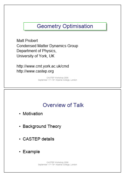
CASTEP Workshop 2006 September 11th-15th Imperial College, London
Density Functional Theory (III)
( "! "! = E' ! + ! ") & ") " "H =E ! ! + ! ") ")
which obviously includes forces and stresses. • We have assumed that the wavefunction is properly normalised and is an exact eigenstate of H.
CASTEP Workshop 2006 September 11th-15th Imperial College, London
Stress and strain in action
c b % # $ a c b b c # $ a!a+&a
"xx
%
# $ a
"xy
% !%+&%
NB Much messier if non-orthogonal cell
– Can therefore minimise enthalpy w.r.t. supercell shape due to internal stress and external pressure – Pressure-driven phase transitions
ansys软件问答合集(二)

47 在Ansys中,碰到提示“Volume 1 cannot be meshed. 208 location(s) found where non-adjacent boundary triangles touch. Geometry configuration may not be valid or smaller element size definition may be required.”。这是什么问题? 回答:提示就是告诉你需要更小的单元,可能单元太大的时候出现的网格有有问题,比如狭长 的网格,计算的时候集中应力太大。
48 在Ansys中,碰到错误Volume11 could not be swept because a source and a target area could not be determined automatically。please try again...,这是什么原因? 回答:体不符合SWEEP的条件,把体修改成比较规则的形状,可以分割试试。 49 在Ansys中,碰到警告和错误:“*** WARNING *** SUPPRESSED MESSAGE CP = 1312.641 TIME= 16:51:48 An error has occurred writing to the file = 12 which may imply a full disk. The system I/O error = 28. Please refer to your system documentation on I/O errors. ”,这是什 么错误和警告? 回答:1.I/O设备口错误,I/O=26,错误,告诉你磁盘已满,让你清理磁盘。但是实际问题的解 决不是这样,是你的磁盘格式不对,将你的磁盘格式从FAT26改称NTFS的就可以了。因为 FAT26格式的要求你的单一文件不能大于4G。但是我们一旦做瞬态或者是谐相应的时候都很 容易超过这个数,所以系统抱错。Байду номын сангаас2.I/O设备口错误,I/O=9,错误,和上一个一样告诉你磁盘已满,让你清理磁盘。但是实际问题 是由于你的磁盘太碎了造成的,你只要进行磁盘碎片整理就可以了,这个问题就迎刃而解。
『论文笔记』SuperGlue
『论⽂笔记』SuperGlue特征处理部分⽐较好理解,点的self、cross注意⼒机制实现建议看下源码(MultiHeadedAttention),def attention(query, key, value):dim = query.shape[1]scores = torch.einsum('bdhn,bdhm->bhnm', query, key) / dim**.5prob = torch.nn.functional.softmax(scores, dim=-1)return torch.einsum('bhnm,bdhm->bdhn', prob, value), probclass MultiHeadedAttention(nn.Module):""" Multi-head attention to increase model expressivitiy """def__init__(self, num_heads: int, d_model: int):super().__init__()assert d_model % num_heads == 0self.dim = d_model // num_headsself.num_heads = num_headsself.merge = nn.Conv1d(d_model, d_model, kernel_size=1)self.proj = nn.ModuleList([deepcopy(self.merge) for _ in range(3)])def forward(self, query, key, value):batch_dim = query.size(0)query, key, value = [l(x).view(batch_dim, self.dim, self.num_heads, -1)for l, x in zip(self.proj, (query, key, value))]x, prob = attention(query, key, value)self.prob.append(prob)return self.merge(x.contiguous().view(batch_dim, self.dim*self.num_heads, -1))这⾥直接跳到最后的逻辑部分,这部分论⽂写的⽐较粗略,需要看下源码才知道在讲啥(也许有⼤佬不⽤看)。
基于生成式对抗网络的画作图像合成方法
收稿日期:2020 03 14;修回日期:2020 05 06 基金项目:国家自然科学基金资助项目(91746107) 作者简介:赵宇欣(1995 ),女,山西晋中人,硕士研究生,主要研究方向为机器学习、深度学习、计算机视觉(zhaoyuxin_alice@tju.edu.cn);王冠(1992 ),女,内蒙古呼伦贝尔人,博士研究生,主要研究方向为深度学习、数学物理反问题.基于生成式对抗网络的画作图像合成方法赵宇欣,王 冠(天津大学数学学院,天津300354)摘 要:画作图像合成旨在将两个不同来源的图像分别作为前景和背景融合在一起,这通常需要局部风格迁移。
现有算法过程繁琐且耗时,不能做到实时的图像合成。
针对这一缺点,提出了基于生成式对抗网络(generativeadversarialnet,GAN)的前向生成模型(PainterGAN)。
PainterGAN的自注意力机制和U Net结构控制合成过程中前景的语义内容不变。
同时,对抗学习保证逼真的风格迁移。
在实验中,使用预训练模型作为PainterGAN的生成器,极大地节省了计算时间和成本。
实验结果表明,比起已有方法,PainterGAN生成了质量相近甚至更好的图像,生成速度也提升了400倍,在解决局部风格迁移问题上是高质量、高效率的。
关键词:图像风格迁移;生成对抗网络;图像合成;自注意力机制中图分类号:TP391 41 文献标志码:A 文章编号:1001 3695(2021)04 047 1208 04doi:10.19734/j.issn.1001 3695.2020.03.0082PainterlyimagecompositionbasedongenerativeadversarialnetZhaoYuxin,WangGuan(SchoolofMathematics,TianjinUniversity,Tianjin300354,China)Abstract:Painterlyimagecompositingaimstoharmonizeaforegroundimageinsertedintoabackgroundpainting,whichisdonebylocalstyletransfer.Thechiefdrawbackoftheexistingmethodsisthehighcomputationalcost,whichmakesreal timeoperationdifficult.Toovercomethisdrawback,thispaperproposedafeed forwardmodelbasedongenerativeadversarialnet work(GAN),calledPainterGAN.PainterGANintroducedaself attentionnetworkandaU Nettocontrolthesemanticcontentinthegeneratedimage.Meanwhile,adversariallearningguaranteedafaithfultransferofstyle.PainterGANalsointroducedapre trainednetworkwithinthegeneratortoextractfeatures.ThisallowedPainterGANtodramaticallyreducetraining timeandstorage.Experimentsshowthat,comparedtostate of artmethods,PainterGANgeneratedimageshundredsoftimesfasterwithcomparableorsuperiorquality.Therefore,itiseffectiveandefficientforlocalstyletransfer.Keywords:imagestyletransfer;GAN;imagecompositing;self attention0 引言图像合成属于图像变换问题,目的是通过模型将一个简单的粘贴合成图像转变成一个融合为一体的图像。
Minimum_Spanning_Tree_Problem早稻田大学PPT
w78=1 ,x78=1 w67=5 ,x67=1
7
w56=6 ,x56=1
w79=4 ,x79=1
9
3
x
| S | 1, S V \{1},| S | 2 : no loop
w49=8 ,x49=1
5
4
xij 0 or 1, i, j 1, 2, ..., n
Soft Computing Lab. WASEDA UNIVERSITY , IPS
4.1 Basic Concept of lc-MST 4.2 Genetic Algorithms Approach 4.3 GA procedure for lc-MST 4.4 Numerical Experiments
Soft Computing Lab.
WASEDA UNIVERSITY , IPS
5
1
8
3 4 7
4
6
6
7
2
9
8
2
3
i
wij
2
j
5
1
4
Fig. 7.1 Example of network model
Table for non-directed graph
Tavakoly., B.: Gene Expression Data Clustering With Minimum Spanning Tree, Department of Information Systems and Computing, Brunel University, May 2003. Soft Computing Lab. WASEDA UNIVERSITY , IPS
3.1 Concept on Degree-based Permutation GA 3.2 Genetic Algorithms Approach 3.3 Degree-based Permutation GA for dc-MST 3.4 Numerical Experiments
【5A文】关于序列二次规划(SQP)算法求解非线性规划问题研究
关于序列二次规划(SQP)算法求解非线性规划问题研究兰州大学硕士学位论文关于序列二次规划(SQP)算法求解非线性规划问题的研究姓名:石国春申请学位级别:硕士专业:数学、运筹学与控制论指导教师:王海明20090602兰州大学2009届硕士学位论文摘要非线性约束优化问题是最一般形式的非线性规划NLP问题,近年来,人们通过对它的研究,提出了解决此类问题的许多方法,如罚函数法,可行方向法,Quadratic及序列二次规划SequentialProgramming简写为SOP方法。
本文主要研究用序列二次规划SOP算法求解不等式约束的非线性规划问题。
SOP算法求解非线性约束优化问题主要通过求解一系列二次规划子问题来实现。
本文基于对大规模约束优化问题的讨论,研究了积极约束集上的SOP 算法。
我们在约束优化问题的s一积极约束集上构造一个二次规划子问题,通过对该二次规划子问题求解,获得一个搜索方向。
利用一般的价值罚函数进行线搜索,得到改进的迭代点。
本文证明了这个算法在一定的条件下是全局收敛的。
关键字:非线性规划,序列二次规划,积极约束集Hl兰州人学2009届硕二t学位论文AbstractNonlinearconstrainedarethemostinoptimizationproblemsgenericsubjectsmathematicalnewmethodsareachievedtosolveprogramming.Recently,Manyasdirectionit,suchfunction,feasiblemethod,sequentialquadraticpenaltyprogramming??forconstrainedInthisthemethodspaper,westudysolvinginequalityabyprogrammingalgorithm.optimizationproblemssequentialquadraticmethodaofSQPgeneratesquadraticprogrammingQPsequencemotivationforthisworkisfromtheofsubproblems.OuroriginatedapplicationsinanactivesetSQPandSQPsolvinglarge-scaleproblems.wepresentstudyforconstrainedestablishontheQPalgorithminequalityoptimization.wesubproblemsactivesetofthesearchdirectionisachievedQPoriginalproblem.AbysolvingandExactfunctionsaslinesearchfunctionsubproblems.wepresentgeneralpenaltyunderobtainabetteriterate.theofourisestablishedglobalconvergencealgorithmsuitableconditions.Keywords:nonlinearprogramming,sequentialquadraticprogrammingalgorithm,activesetlv兰州大学2009届硕士学位论文原创性声明本人郑重声明:本人所呈交的学位论文,是在导师的指导下独立进行研究所取得的成果。
- 1、下载文档前请自行甄别文档内容的完整性,平台不提供额外的编辑、内容补充、找答案等附加服务。
- 2、"仅部分预览"的文档,不可在线预览部分如存在完整性等问题,可反馈申请退款(可完整预览的文档不适用该条件!)。
- 3、如文档侵犯您的权益,请联系客服反馈,我们会尽快为您处理(人工客服工作时间:9:00-18:30)。
ApproximateConstrainedSubgraphMatchingSt´ephaneZampelli,YvesDeville,andPierreDupontUniversit´eCatholiquedeLouvain,DepartmentofComputingScienceandEngineering,2,PlaceSainte-Barbe1348Louvain-la-Neuve(Belgium)sz,yde,pdupont@info.ucl.ac.be
1IntroductionOurgoalistobuildadeclarativeframeworkforapproximategraphmatchingwherevariousconstraintscanbestateduponthepatterngraph,enablingapproximatecon-strainedsubgraphmatching,extendingmodelsandconstraintsproposedbyRudolf[1]andValienteetal.[2].Inthepresentwork,weproposeaCSPapproachforapproximatesubgraphmatchingwherethepotentialapproximationisdeclarativelystatedinthepat-terngraphasmandatory/optionalnodes/edges.Forbiddenedges,thatisedgesthatmaynotbeincludedinthematching,canbedeclaredonthepatterngraph.Wealsowanttodeclarepropertiesbetweenpairsofnodesinthepatterngraph,suchasdistanceprop-erties,thatcanbeeitherstatedbytheuser,orautomaticallyinferredbythesystem.Intheformercase,suchpropertiescandefinenewapproximatepatterns.Inthelattercase,theseredundantconstraintsenhancethepruning.
2ApproximateSubgraphMatching2.1ProblemDefinitionAsubgraphmonomorphismbetweenapatterngraphandatargetgraphisaninjectivefunctionrespecting.Aconstraintmodeltosolvetheexactsubgraphmatchingproblemhasbeenproposedbyseveralauthors[2][1].Thismodelfocusesonmonomorphismandwillformourbasicmonomorphismconstraints.Thevariablesarethenodesofthepatterngraphandtheirrespectivedomainisthesetoftar-getnodes.Theassignmentmustrespecttwoconditions:allvariableshaveadifferentvalueandthestructureofthepatternmustbekept(monomorphismcondition).InaCSPframework,thefirstconditionisimplementedwiththeclassicalAlldiffconstraint[3][4].Thesecondconditionistranslatedintoamonomorphismconstraint.Ausefulextensionofsubgraphmatchingisapproximatesubgraphmatching,wherethepatterngraphandthefoundsubgraphinthetargetgraphmaydifferwithrespecttotheirstructure.2ZampelliSt´ephaneetal.OptionalnodesInourframework,theapproximationisdeclareduponthepatterngraph.Somenodesaredeclaredoptional,i.e.nodesthatmaynotbeinthematching.Specifyingoptionaledgesinamonomorphismproblemisuselessasitisequivalenttoomittingtheedgeinthepattern.Thestatusoftheedgesdependsontheoptionalstateoftheirendpoints.Anedgehavinganoptionalnodeasoneofitsendpointsisoptional.Anoptionaledgeisnotconsideredinthematchingifoneofitsendpointsisnotpartofthematching.Otherwise,theedgemustalsobeapartofthematching.ForbiddenedgesEdgesmayalsobedeclaredasforbiddenbetweentheirtwoend-points,meaningthatifandareinthedomainof,thenmustnotexistinthetargetgraph.Apatterngraphwithallitscomplementaryedgesdeclaredasforbiddeninducesasubgraphisomorphisminsteadofasubgraphmonomorphism.Apatterngraphwithoptionalnodesandforbiddenedgesformsanapproximatepatterngraph.
Definition1Anapproximatepatterngraphisatuplewhereisagraph,isthesetofoptionalnodesandisthesetoffor-biddenedges,with.
Thecorrespondingmatchingiscalledanapproximatesubgraphmatching.Definition2Anapproximatesubgraphmatchingbetweenanapproximatepatterngraphandatargetgraphisapartialfunc-tionsuchthat:
1.2.3.4.
Thenotationrepresentsthedomainof.Elementsofarecalledtheselectednodesofthematching.Thismeansthatcanberepresentedbyafinitesetvariable.Itslowerboundconsistsofallselectednodes,anditsupperboundconsistsofselectednodesandnodesthatcouldbeselected.
3ConstraintsforApproximateSubgraphMatching
AlldiffConstraintTheAlldiffconstraintmustbeadaptedtovariablesthatmaynotbeassigned.Onesolutionistocreatesymbolicvaluesandputintheinitialdomainof.Inasolution,ifisnotassignedtoanytargetnode.Usingthesesymbolicvalues,aglobalAlldiffconstraintcanstillbepostedasintheexactcase.MorphismConstraintThebasicmorphismconditionforcingthematchingtorespectthepatternstructure(see[2])hasbeengeneralizedtohandlemoregeneralmorphismconditionsaswellasoptionalnodes:
Theformerconstraintstatesthatamorphismrelationbetweentwopatternnodesandmustbeforcedifandonlyiftheyarepresentinthedomainof.Theconstraint
canberewrittenas:ApproximateConstrainedSubgraphMatching3Theproposedpropagatorkeepstrackofrelationsbetweenallthetargetnodesandthedomaininastructurerepresentingthenumberofrelationsbetweenatargetnodeand(see[2]).Theadditionalconditionstatesthatonlyselectednodesshouldpropagateunderthemorphismcondition.Thepropagationofthemorphismconstraintofanoptionaliscomputedbutperformedonlywhenisinthedomainof.AsdepictedinFigure1,allselectednodespropagateintheirneighborhoodbutoptionalnodespropagateonlywhentheyareselected.
Fig.1.PruningmethodfortheapproximatemorphismconditionForbiddenEdgesConstraintAconstraintfortheforbiddenedges(condition4inthematching)canbeobtainedbyparameterizingwith