2 Thermodynamics-based constitutive framework for unsaturated soils 2
框架结构外文文献

Seismic Collapse Safety of Reinforced ConcreteBuildings.II:Comparative Assessment of Nonductile and Ductile Moment FramesAbbie B.Liel,M.ASCE 1;Curt B.Haselton,M.ASCE 2;and Gregory G.Deierlein,F.ASCE 3Abstract:This study is the second of two companion papers to examine the seismic collapse safety of reinforced concrete frame buildings,and examines nonductile moment frames that are representative of those built before the mid-1970s in California.The probabilistic assessment relies on nonlinear dynamic simulation of structural response to calculate the collapse risk,accounting for uncertainties in ground-motion characteristics and structural modeling.The evaluation considers a set of archetypical nonductile RC frame structures of varying height that are designed according to the seismic provisions of the 1967Uniform Building Code.The results indicate that nonductile RC frame structures have a mean annual frequency of collapse ranging from 5to 14×10À3at a typical high-seismic California site,which is approximately 40times higher than corresponding results for modern code-conforming special RC moment frames.These metrics demonstrate the effectiveness of ductile detailing and capacity design requirements,which have been introduced over the past 30years to improve the safety of RC buildings.Data on comparative safety between nonductile and ductile frames may also inform the development of policies for appraising and mitigating seismic collapse risk of existing RC frame buildings.DOI:10.1061/(ASCE)ST.1943-541X .0000275.©2011American Society of Civil Engineers.CE Database subject headings:Structural failures;Earthquake engineering;Structural reliability;Reinforced concrete;Concrete structures;Seismic effects;Frames.Author keywords:Collapse;Earthquake engineering;Structural reliability;Reinforced concrete structures;Buildings;Commercial;Seismic effects.IntroductionReinforced concrete (RC)frame structures constructed in Califor-nia before the mid-1970s lack important features of good seismic design,such as strong columns and ductile detailing of reinforce-ment,making them potentially vulnerable to earthquake-induced collapse.These nonductile RC frame structures have incurred significant earthquake damage in the 1971San Fernando,1979Imperial Valley,1987Whittier Narrows,and 1994Northridge earthquakes in California,and many other earthquakes worldwide.These factors raise concerns that some of California ’s approxi-mately 40,000nonductile RC structures may present a significant hazard to life and safety in future earthquakes.However,data are lacking to gauge the significance of this risk,in relation to either the building population at large or to specific buildings.The collapse risk of an individual building depends not only on the building code provisions employed in its original design,but also structuralconfiguration,construction quality,building location,and site-spe-cific seismic hazard information.Apart from the challenges of ac-curately evaluating the collapse risk is the question of risk tolerance and the minimum level of safety that is appropriate for buildings.In this regard,comparative assessment of buildings designed accord-ing to old versus modern building codes provides a means of evalu-ating the level of acceptable risk implied by current design practice.Building code requirements for seismic design and detailing of reinforced concrete have changed significantly since the mid-1970s,in response to observed earthquake damage and an in-creased understanding of the importance of ductile detailing of reinforcement.In contrast to older nonductile RC frames,modern code-conforming special moment frames for high-seismic regions employ a variety of capacity design provisions that prevent or delay unfavorable failure modes such as column shear failure,beam-column joint failure,and soft-story mechanisms.Although there is general agreement that these changes to building code require-ments are appropriate,there is little data to quantify the associated improvements in seismic safety.Performance-based earthquake engineering methods are applied in this study to assess the likelihood of earthquake-induced collapse in archetypical nonductile RC frame structures.Performance-based earthquake engineering provides a probabilistic framework for re-lating ground-motion intensity to structural response and building performance through nonlinear time-history simulation (Deierlein 2004).The evaluation of nonductile RC frame structures is based on a set of archetypical structures designed according to the pro-visions of the 1967Uniform Building Code (UBC)(ICBO 1967).These archetype structures are representative of regular well-designed RC frame structures constructed in California between approximately 1950and 1975.Collapse is predicted through1Assistant Professor,Dept.of Civil,Environmental and Architectural Engineering,Univ.of Colorado,Boulder,CO 80309.E-mail:abbie .liel@ 2Assistant Professor,Dept.of Civil Engineering,California State Univ.,Chico,CA 95929(corresponding author).E-mail:chaselton@csuchico .edu 3Professor,Dept.of Civil and Environmental Engineering,Stanford Univ.,Stanford,CA 94305.Note.This manuscript was submitted on July 14,2009;approved on June 30,2010;published online on July 15,2010.Discussion period open until September 1,2011;separate discussions must be submitted for individual papers.This paper is part of the Journal of Structural Engineer-ing ,V ol.137,No.4,April 1,2011.©ASCE,ISSN 0733-9445/2011/4-492–502/$25.00.492/JOURNAL OF STRUCTURAL ENGINEERING ©ASCE /APRIL 2011D o w n l o a d e d f r o m a s c e l i b r a r y .o r g b y S u l t a n Q a b o o s U n i v e r s i t y o n 06/21/14. C o p y r i g h t A S CE .F o r p e r s o n a l u s e o n l y ; a l l r i g h t s r e s e r v e d .nonlinear dynamic analysis of the archetype nonductile RC frames,using simulation models capable of capturing the critical aspects of strength and stiffness deterioration as the structure collapses.The outcome of the collapse performance assessment is a set of measures of building safety and relating seismic collapse resistance to seismic hazard.These results are compared with the metrics for ductile RC frames reported in a companion paper (Haselton et al.2011b ).Archetypical Reinforced Concrete Frame StructuresThe archetype nonductile RC frame structures represent the expected range in design and performance in California ’s older RC frame buildings,considering variations in structural height,configuration and design details.The archetype configurations explore key design parameters for RC components and frames,which were identified through previous analytical and experimental studies reviewed by Haselton et al.(2008).The complete set of archetype nonductile RC frame buildings developed for this study includes 26designs (Liel and Deierlein 2008).This paper focuses primarily on 12of these designs,varying in height from two to 12stories,and including both perimeter (P )and space (S )frame lateral resisting systems with alternative design details.All archetype buildings are designed for office occupancies with an 8-in.(20-cm)flat-slab floor system and 25-ft (7.6-m)column spacing.The 2-and 4-story buildings have a footprint of 125ft by 175ft (38.1m by 53.3m),and the 8-and 12-story buildings measure 125ft (38.1m)square in plan.Story heights are 15ft (4.6m)in the first story and 13ft (4.0m)in all other stories.Origi-nal structural drawings for RC frame buildings constructed in California in the 1960s were used to establish typical structural configurations and geometry for archetype structures (Liel and Deierlein 2008).The archetypes are limited to RC moment frames without infill walls,and are regular in elevation and plan,without major strength or stiffness irregularities.The nonductile RC archetype structures are designed for the highest seismic zone in the 1967UBC,Zone 3,which at that time included most of California.Structural designs of two-dimensional frames are governed by the required strength and stiffness to satisfy gravity and seismic loading combinations.The designs also satisfy all relevant building code requirements,including maximum and minimum reinforcement ratios and maximum stirrup spacing.The 1967UBC permitted an optional reduction in the design base shear if ductile detailing requirements were employed,however,this reduction is not applied and only standard levels of detailing are considered in this study.Design details for each structure areTable 1.Design Characteristics of Archetype Nonductile and Ductile RC Frames Stucture Design base shear coefficient a,bColumn size c (in :×in.)Column reinforcementratio,ρColumn hoop spacing d,e (in.)Beam size f (in :×in.)Beam reinforcementratios ρ(ρ0)Beam hoop spacing (in.)Nonductile2S 0.08624×240.0101224×240.006(0.011)112P 0.08630×300.0151530×300.003(0.011)114S 0.06820×200.0281020×260.007(0.014)124P 0.06824×280.0331424×320.007(0.009)158S 0.05428×280.0141424×260.006(0.013)118P 0.05430×360.0331526×360.008(0.010)1712S 0.04732×320.025926×300.006(0.011)1712P 0.04732×400.032930×380.006(0.013)184S g 0.06820×200.028 6.720×260.007(0.014)84S h 0.06820×200.0281020×260.007(0.014)1212S g 0.04732×320.025626×300.006(0.011)1112S h 0.04732×320.025926×300.006(0.011)17Ductile2S 0.12522×220.017518×220.006(0.012) 3.52P 0.12528×300.018528×280.007(0.008)54S 0.09222×220.016522×240.004(0.008)54P 0.09232×380.016 3.524×320.011(0.012)58S 0.05022×220.011422×220.006(0.011) 4.58P 0.05026×340.018 3.526×300.007(0.008)512S 0.04422×220.016522×280.005(0.008)512P0.04428×320.0223.528×380.006(0.007)6aThe design base shear coefficient in the 1967UBC is given by C ¼0:05=T ð1=3Þ≤0:10.For moment resisting frames,T ¼0:1N ,where N is the number of stories (ICBO 1967).bThe design base shear coefficient for modern buildings depends on the response spectrum at the site of interest.The Los Angeles site has a design spectrumdefined by S DS ¼1:0g and S D1¼0:60g.The period used in calculation of the design base shear is derived from the code equation T ¼0:016h 0:9n ,where h n isthe height of the structure in feet,and uses the coefficient for upper limit of calculated period (C u ¼1:4)(ASCE 2002).cColumn properties vary over the height of the structure and are reported here for an interior first-story column.dConfiguration of transverse reinforcement in each member depends on the required shear strength.There are at least two No.3bars at every location.eConfiguration of transverse reinforcement in ductile RC frames depends on the required shear strength.All hooks have seismic detailing and use No.4bars (ACI 2005).fBeam properties vary over the height of the structure and are reported here are for a second-floor beam.gThese design variants have better-than-average beam and column detailing.hThese design variants have better-than-average joint detailing.JOURNAL OF STRUCTURAL ENGINEERING ©ASCE /APRIL 2011/493D o w n l o a d e d f r o m a s c e l i b r a r y .o r g b y S u l t a n Q a b o o s U n i v e r s i t y o n 06/21/14. C o p y r i g h t A S CE .F o r p e r s o n a l u s e o n l y ; a l l r i g h t s r e s e r v e d .summarized in Table 1,and complete documentation of the non-ductile RC archetypes is available in Liel and Deierlein (2008).Four of the 4-and 12-story designs have enhanced detailing,as described subsequently.The collapse performance of archetypical nonductile RC frame structures is compared to the set of ductile RC frame archetypes presented in the companion paper (Haselton et al.2011b ).As sum-marized in Table 2,these ductile frames are designed according to the provisions of the International Building Code (ICC 2003),ASCE 7(ASCE 2002),and ACI 318(ACI 2005);and meet all gov-erning code requirements for strength,stiffness,capacity design,and detailing for special moment frames.The structures benefit from the provisions that have been incorporated into seismic design codes for reinforced concrete since the 1970s,including an assort-ment of capacity design provisions [e.g.,strong column-weak beam (SCWB)ratios,beam-column and joint shear capacity design]and detailing improvements (e.g.,transverse confinement in beam-column hinge regions,increased lap splice requirements,closed hooks).The ductile RC frames are designed for a typical high-seismic Los Angeles site with soil class S d that is located in the transition region of the 2003IBC design maps (Haselton and Deierlein 2007).A comparison of the structures described in Table 1reflects four decades of changes to seismic design provisions for RC moment frames.Despite modifications to the period-based equation for design base shear,the resulting base shear coefficient is relatively similar for nonductile and ductile RC frames of the same height,except in the shortest structures.More significant differencesbetween the two sets of buildings are apparent in member design and detailing,especially in the quantity,distribution,and detailing of transverse reinforcement.Modern RC frames are subject to shear capacity design provisions and more stringent limitations on stirrup spacing,such that transverse reinforcement is spaced two to four times more closely in ductile RC beams and columns.The SCWB ratio enforces minimum column strengths to delay the formation of story mechanisms.As a result,the ratio of column to beam strength at each joint is approximately 30%higher (on average)in the duc-tile RC frames than the nonductile RC frames.Nonductile RC frames also have no special provision for design or reinforcement of the beam-column joint region,whereas columns in ductile RC frames are sized to meet joint shear demands with transverse reinforcement in the joints.Joint shear strength requirements in special moment frames tend to increase the column size,thereby reducing axial load ratios in columns.Nonlinear Simulation ModelsNonlinear analysis models for each archetype nonductile RC frame consist of a two-dimensional three-bay representation of the lateral resisting system,as shown in Fig.1.The analytical model repre-sents material nonlinearities in beams,columns,beam-column joints,and large deformation (P -Δ)effects that are important for simulating collapse of frames.Beam and column ends and the beam-column joint regions are modeled with member end hinges that are kinematically constrained to represent finite joint sizeTable 2.Representative Modeling Parameters in Archetype Nonductile and Ductile RC Frame Structures Structure Axial load a,b (P =A g f 0c )Initial stiffness c Plastic rotation capacity (θcap ;pl ,rad)Postcapping rotation capacity (θpc ,rad)Cyclicdeterioration d (λ)First mode period e (T 1,s)Nonductile2S 0.110:35EI g 0.0180.04041 1.12P 0.030:35EI g 0.0170.05157 1.04S 0.300:57EI g 0.0210.03333 2.04P 0.090:35EI g 0.0310.10043 2.08S 0.310:53EI g 0.0130.02832 2.28P 0.110:35EI g 0.0250.10051 2.412S 0.350:54EI g 0.0290.06353 2.312P 0.140:35EI g 0.0450.10082 2.84S f 0.300:57EI g 0.0320.04748 2.04S g 0.300:57EI g 0.0210.03333 2.012S f 0.350:54EI g 0.0430.09467 2.312S g 0.350:54EI g 0.0290.06353 2.3Ductile2S 0.060:35EI g 0.0650.100870.632P 0.010:35EI g 0.0750.1001110.664S 0.130:38EI g 0.0570.100800.944P 0.020:35EI g 0.0860.100133 1.18S 0.210:51EI g 0.0510.10080 1.88P 0.060:35EI g 0.0870.100122 1.712S 0.380:68EI g 0.0360.05857 2.112P0.070:35EI g0.0700.1001182.1a Properties reported for representative interior column in the first story.(Column model properties data from Haselton et al.2008.)bExpected axial loads include the unfactored dead load and 25%of the design live load.cEffective secant stiffness through 40%of yield strength.dλis defined such that the hysteretic energy dissipation capacity is given by Et ¼λM y θy (Haselton et al.2008).eObtained from eigenvalue analysis of frame model.fThese design variants have better-than-average beam and column detailing.gThese design variants have better-than-average joint detailing.494/JOURNAL OF STRUCTURAL ENGINEERING ©ASCE /APRIL 2011D o w n l o a d e d f r o m a s c e l i b r a r y .o r g b y S u l t a n Q a b o o s U n i v e r s i t y o n 06/21/14. C o p y r i g h t A S CE .F o r p e r s o n a l u s e o n l y ; a l l r i g h t s r e s e r v e d .effects and connected to a joint shear spring (Lowes and Altoontash 2003).The structural models do not include any contribution from nonstructural components or from gravity-load resisting structural elements that are not part of the lateral resisting system.The model is implemented in OpenSees with robust convergence algorithms (OpenSees 2009).As in the companion paper,inelastic beams,columns,and joints are modeled with concentrated springs idealized by a trilinear back-bone curve and associated hysteretic rules developed by Ibarra et al.(2005).Properties of the nonlinear springs representing beam and column elements are predicted from a series of empirical relation-ships relating column design characteristics to modeling parame-ters and calibrated to experimental data for RC columns (Haselton et al.2008).Tests used to develop empirical relationships include a large number of RC columns with nonductile detailing,and predicted model parameters reflect the observed differences in moment-rotation behavior between nonductile and ductile RC elements.As in the companion paper,calibration of model param-eters for RC beams is established on columns tested with low axial load levels because of the sparse available beam data.Fig.2(a)shows column monotonic backbone curve properties for a ductile and nonductile column (each from a 4-story building).The plastic rotation capacity θcap ;pl ,which is known to have an important influence on collapse prediction,is a function of the amount of column confinement reinforcement and axial load levels,and is approximately 2.7times greater for the ductile RC column.The ductile RC column also has a larger postcapping rotation capacity (θpc )that affects the rate of postpeak strength degradation.Fig.2(b)illustrates cyclic deterioration of column strength and stiffness under a typical loading protocol.Cyclic degradation of the initial backbone curve is controlled by the deterioration parameter λ,which is a measure of the energy dissipation capacity and is smaller in nonductile columns because of poor confinement and higher axial loads.Model parameters are calibrated to the expected level of axial compression in columns because of gravity loads and do not account for axial-flexure-shear interaction during the analysis,which may be significant in taller buildings.Modeling parameters for typical RC columns in nonductile and ductile archetypes are summarized in Table 2.Properties for RC beams are similar and reported elsewhere (Liel and Deierlein 2008;Haselton and Deierlein 2007).All element model properties are calibrated to median values of test data.Although the hysteretic beam and column spring parameters incorporate bond-slip at the member ends,they do not account for significant degradations that may occur because of anchorage or splice failure in nonductile frames.Unlike ductile RC frames,in which capacity design require-ments limit joint shear deformations,nonductile RC frames may experience significant joint shear damage contributing to collapse (Liel and Deierlein 2008).Joint shear behavior is modeled with an inelastic spring,as illustrated in Fig.1and defined by a monotonic backbone and hysteretic rules (similar to those shown in Fig.2for columns).The properties of the joint shear spring are on the basisofFig.1.Schematic of the RC frame structural analysismodel(a)(b)Fig.2.Properties of inelastic springs used to model ductile and non-ductile RC columns in the first story of a typical 4-story space frame:(a)monotonic behavior;(b)cyclic behaviorJOURNAL OF STRUCTURAL ENGINEERING ©ASCE /APRIL 2011/495D o w n l o a d e d f r o m a s c e l i b r a r y .o r g b y S u l t a n Q a b o o s U n i v e r s i t y o n 06/21/14. C o p y r i g h t A S CE .F o r p e r s o n a l u s e o n l y ; a l l r i g h t s r e s e r v e d .selected subassembly data of joints with minimal amounts of trans-verse reinforcement and other nonductile characteristics.Unfortu-nately,available data on nonconforming joints are limited.Joint shear strength is computed using a modified version of the ACI 318equation (ACI 2005),and depends on joint size (b j is joint width,h is height),concrete compressive strength (f 0c ,units:psi),and confinement (γ,which is 12to 20depending on the configu-ration of confining beams)such that V ¼0:7γffiffiffiffif 0c p b j h .The 0.7modification factor is on the basis of empirical data from Mitra and Lowes (2007)and reflects differences in shear strength between seismically detailed joints (as assumed in ACI 318Chap.21)and joints without transverse reinforcement,of the type consid-ered in this study.Unlike conforming RC joints,which are assumed to behave linear elastically,nonductile RC joints have limited duc-tility,and shear plastic deformation capacity is assumed to be 0.015and 0.010rad for interior and exterior joints,respectively (Moehle et al.2006).For joints with axial load levels below 0.095,data from Pantelides et al.(2002)are used as the basis for a linear increase in deformation capacity (to a maximum of 0.025at zero axial load).Limited available data suggest a negative postcapping slope of approximately 10%of the effective initial stiffness is appropriate.Because of insubstantial data,cyclic deterioration properties are assumed to be the same as that for RC beams and columns.The calculated elastic fundamental periods of the RC frame models,reported in Table 2,reflect the effective “cracked ”stiffness of the beams and columns (35%of EI g for RC beams;35%to 80%of EI g for columns),finite joint sizes,and panel zone flexibility.The effective member stiffness properties are determined on the basis of deformations at 40%of the yield strength and include bond-slip at the member ends.The computed periods are signifi-cantly larger than values calculated from simplified formulas in ASCE (2002)and other standards,owing to the structural modeling assumptions (specifically,the assumed effective stiffness and the exclusion of the gravity-resisting system from the analysis model)and intentional conservatism in code-based formulas for building period.Nonlinear static (pushover)analysis of archetype analysis mod-els shows that the modern RC frames are stronger and have greater deformation capacities than their nonductile counterparts,as illus-trated in Fig.3.The ASCE 7-05equivalent seismic load distribu-tion is applied in the teral strength is compared on the basis of overstrength ratio,Ω,defined as the ratio between the ultimate strength and the design base shear.The ductility is com-pared on the basis of ultimate roof drift ratio (RDR ult ),defined as the roof drift ratio at which 20%of the lateral strength of the structure has been lost.As summarized in Table 3,for the archetype designs in this study,the ductile RC frames have approximately 40%more overstrength and ultimate roof drift ratios three times larger than the nonductile RC frames.The larger structural deformation capacity and overstrength in the ductile frames results from (1)greater deformation capacity in ductile versus nonductile RC components (e.g.,compare column θcap ;pl and θpc in Table 2),(2)the SCWB requirements that promote more distributed yielding over multiple stories in the ductile frames,(3)the larger column strengths in ductile frames that result from the SCWB and joint shear strength requirements,and (4)the required ratios of positive and negative bending strength of the beams in the ductile frames.Fig.3(b)illustrates the damage concentration in lower stories,especially in the nonductile archetype structures.Whereas nonlin-ear static methods are not integral to the dynamic collapse analyses,the pushover results help to relate the dynamic collapse analysis results,described subsequently,and codified nonlinear static assessment procedures.Collapse Performance Assessment ProcedureSeismic collapse performance assessment for archetype nonductile RC frame structures follows the same procedure as in the companion study of ductile RC frames (Haselton et al.2011b ).The collapse assessment is organized using incremental dynamic analysis (IDA)of nonlinear simulation models,where each RC frame model is subjected to analysis under multiple ground motions that are scaled to increasing amplitudes.For each ground motion,collapse is defined on the basis of the intensity (spectral acceleration at the first-mode period of the analysis model)of the input ground motion that results in structural collapse,as iden-tified in the analysis by excessive interstory drifts.The IDA is repeated for each record in a suite of 80ground motions,whose properties along with selection and scaling procedures are de-scribed by Haselton et al.(2011b ).The outcome of this assessment is a lognormal distribution (median,standard deviation)relating that structure ’s probability of collapse to the ground-motion inten-sity,representing a structural collapse fragility function.Uncer-tainty in prediction of the intensity at which collapse occurs,termed “record-to-record ”uncertainty (σln ;RTR ),is associated with variation in frequency content and other characteristics of ground-motion records.Although the nonlinear analysis model for RC frames can simulate sidesway collapse associated with strength and stiffness degradation in the flexural hinges of the beams andcolumnsFig.3.Pushover analysis of ductile and nonductile archetype 12-story RC perimeter frames:(a)force-displacement response;and (b)distri-bution of interstory drifts at the end of the analysis496/JOURNAL OF STRUCTURAL ENGINEERING ©ASCE /APRIL 2011D o w n l o a d e d f r o m a s c e l i b r a r y .o r g b y S u l t a n Q a b o o s U n i v e r s i t y o n 06/21/14. C o p y r i g h t A S CE .F o r p e r s o n a l u s e o n l y ; a l l r i g h t s r e s e r v e d .and beam-column joint shear deformations,the analysis model does not directly capture column shear failure.The columns in the archetype buildings in this study are expected to yield first in flexure,followed by shear failure (Elwood and Moehle 2005)rather than direct shear failure,as may be experienced by short,squat nonductile RC columns.However,observed earthquake damage and laboratory studies have shown that shear failure and subsequent loss of gravity-load-bearing capacity in one column could lead to progressive collapse in nonductile RC frames.Column shear failure is not incorporated directly because of the difficulties in accurately simulating shear or flexure-shear failure and subsequent loss of axial load-carrying capacity (Elwood 2004).Collapse modes related to column shear failure are therefore detected by postprocessing dynamic analysis results using compo-nent limit state ponent limit state functions are devel-oped from experimental data on nonductile beam-columns and predict the median column drift ratio (CDR)at which shear failure,and the subsequent loss of vertical-load-carrying capacity,will occur.Here,CDR is defined similarly to interstory drift ratio,but excludes the contribution of beam rotation and joint deforma-tion to the total drift because the functions are established on data from column component tests.Component fragility relationships for columns failing in flexure-shear developed by Aslani and Miranda (2005),building on work by Elwood (2004),are employed in this study.For columns with nonductile shear design and detailing in this study and axial load ratios of P =A g f 0c between 0.03and 0.35,Aslani and Miranda (2005)predict that shear failure occurs at a median CDR between 0.017and 0.032rad,depending on the properties of the column,and the deformation capacity decreases with increasing axial load.Sub-sequent loss of vertical-carrying capacity in a column is predicted to occur at a median CDR between 0.032and 0.10rad,again depending on the properties of the column.Since the loss of vertical-load-carrying capacity of a column may precipitate progressive structure collapse,this damage state is defined as collapse in this assessment.In postprocessing dynamic analysis results,the vertical collapse limit state is reached if,during the analysis,the drift in any column exceeds the median value of that column ’s component fragility function.If the vertical collapse mode is predicted to occur at a smaller ground-motion intensity than the sidesway collapse mode (for a particular record),then the collapse statistics are updated.This simplified approach can be shown to give comparable median results to convolving the probability distribution of column drifts experienced as a function of ground-motion intensity (engineering demands)with the com-ponent fragility curve (capacity).The total uncertainty in the col-lapse fragility is assumed to be similar in the sidesway-only case and the sidesway/axial collapse case,as it is driven by modeling and record-to-record uncertainties rather than uncertainty in the component fragilities.Incorporating this vertical collapse limit state has the effect of reducing the predicted collapse capacity of the structure.Fig.4illustrates the collapse fragility curves for the 8-story RC space frame,with and without consideration of shear failure and axial failure following shear.As shown,if one considers collapse to occur with column shear failure,then the collapse fragility can reduce considerably compared to the sidesway collapse mode.However,if one assumes that shear failure of one column does not constitute collapse and that collapse is instead associated with the loss in column axial capacity,then the resulting collapse capac-ity is only slightly less than calculations for sidesway alone.For the nonductile RC frame structures considered in this study,the limit state check for loss of vertical-carrying capacity reduces the median collapse capacity by 2%to 30%as compared to the sidesway collapse statistics that are computed without this check (Liel and Deierlein 2008).Table 3.Results of Collapse Performance Assessment for Archetype Nonductile and Ductile RC Frame Structures Structure ΩRDR ult Median Sa ðT 1Þ(g)Sa 2=50ðT 1Þ(g)Collapse marginλcollapse ×10À4IDR collapse RDR collapseNonductile 2S 1.90.0190.470.800.591090.0310.0172P 1.60.0350.680.790.85470.0400.0284S 1.40.0160.270.490.541070.0540.0284P 1.10.0130.310.470.661000.0370.0178S 1.60.0110.290.420.68640.0420.0118P 1.10.0070.230.310.751350.0340.00912S 1.90.0100.290.350.83500.0340.00612P 1.10.0050.240.420.561190.0310.0064S a 1.40.0160.350.490.72380.0560.0244S b 1.60.0180.290.490.60890.0610.02612S a 1.90.0120.330.350.93350.0390.00912S b 2.20.0120.460.351.32160.0560.012Ductile 2S 3.50.085 3.55 1.16 3.07 1.00.0970.0752P 1.80.0672.48 1.13 2.193.40.0750.0614S 2.70.047 2.220.87 2.56 1.70.0780.0504P 1.60.038 1.560.77 2.04 3.60.0850.0478S 2.30.028 1.230.54 2.29 2.40.0770.0338P 1.60.023 1.000.57 1.77 6.30.0680.02712S 2.10.0220.830.44 1.914.70.0550.01812P1.70.0260.850.471.845.20.0530.016a These design variants have better-than-average beam and column detailing.bThese design variants have better-than-average joint detailing.JOURNAL OF STRUCTURAL ENGINEERING ©ASCE /APRIL 2011/497D o w n l o a d e d f r o m a s c e l i b r a r y .o r g b y S u l t a n Q a b o o s U n i v e r s i t y o n 06/21/14. C o p y r i g h t A S CE .F o r p e r s o n a l u s e o n l y ; a l l r i g h t s r e s e r v e d .。
An Elastoplastic Damage Constitutive Model for Concrete

170
LIU Jun et al. / China Ocean Eng., 27(2), 2013, 169 − 182
account. As well known, the irreversible deformation in concrete is closely related to microcracks. The growth and coalescence of microcracks lead to the degradation of stiffness and strength, while interfaces deterioration of microcracks results in incomplete closure after unloading. Therefore, these two theories should be combined, as have been researched by many scholars in various ways. In their research, plasticity can be described in effective stress space (weak coupling) (Lee and Fenves, 1998; Jason et al., 2006), or nominal stress space (strong coupling) (Lubliner et al., 1989; Salari et al., 2004; Kratzig and Polling, 2004), while damage can be described based on isotropic (scalar) (Mazars and Pijaudier-Cabot, 1989; Hassler-Combe and Hartig, 2008) or anisotropic (tensor) (Skrzypek and Ganczarski,1998; Meschke et al., 1998; Voyiadjis et al., 2008) idealization. In order to enhance the numerical efficiency and reflect the nonlinear feature of concrete as well as possible, in the presented research, plasticity is formulated in effective stress space, and isotropic hardening has been taken into account. Besides that, two scalar indicators of tensile damage and compressive damage are introduced to establish strict constitutive model that ensure thermodynamic consistency in describing the different features of concrete under tension and compression. Fully implicit backward-Euler integration algorithm characterized by unconditional stability is employed in the numerical computation. The proposed model is examined firstly by using uniaxial, biaxial and triaxial loading cases, monotonically as well as cyclically. And then, damage process of a double-edge-notched specimen subjected to loading combination of shear and tension is simulated to further verify the model. The tensor product and contractions in this paper are operated by using notational convention as
饱和黄土的性质与非饱和黄土流变模型

第7期
吴燕开等
饱和黄土的性质与非饱和黄土流变模型
1145
(2) 软黄土的容许承载力 目前 尚未有评价软黄土容许承载力的规范可 循 在湿陷性黄土地基规范中 将软黄土 一般饱 和黄土及过渡性质的黄土合而为一 统一根据指标 的好坏来确定饱和黄土的承载力 对于西安市区软黄土的容许承载力的研究 陕 西省某勘察设计院在西安市区进行了大量的静力触 探与荷载试验的对比试验 提出用下面回归方程来 确定西安地区软黄土的容许承载力
ve σ =σ p +η ε + EB ε B ∂t P = σ s + Bε ve
[R ]= 43.12 + 0< 2 450 ( kPa ) 相关系数 r = 0.829 式中 Ps 为单桥静力触探比贯入阻力 由于软黄土力学性质较差 常呈透镜体分布 其厚度常随地下位的抬升而变厚 随地下水位的下 降而变薄 并且软黄土常具有较强的触变性 因此 软黄土地基是建筑物发生变形和破坏的重要因素 应在工程勘察中查清其分布规律和埋藏条件以及地 下水位变化可能造成的影响 使软黄土对建筑物的 破坏尽量减到最低限度
/ MPa-1
0.26
Es / MPa 2.85 6.76 3.1 7.5 4.2 8.7
IL 1.37 0.83 1.42 0.84 0.94 0.51
f k / kPa 80 150 75 150 90 120
层底深度 14 17 18 10.6 7.5 14.5
/m
0.85
0.64 0.24 0.44 0.19
当外加荷载小于黄土的结构强度 σ s 时 组件 D 表现为刚性体 不发生变形 当外加荷载 σ 大于或 等于黄土的结构强度 σ s 时 外力 σ 则克服摩擦组件 的阻力开始滑动 同时黄土结构破坏以后 表现有 一定加功硬化特征 开尔文体发生粘弹性变形 并 随着时间的增加而增大 用力学表达式可以表示为 (1) 当 σ < σ s 非饱和黄土的结构未发生破坏时 σ = EAε A =σ p ( σ p 为摩擦组件 P 中的应力) = ε ε A (2) 当 σ > σ s 形但未破坏时
软土地层中压入式沉井下沉的土塞效应及其影响

DOI: 10.3785/j.issn.1008-973X.2020.07.017软土地层中压入式沉井下沉的土塞效应及其影响易琼1,廖少明1,朱继文2,徐伟忠2(1. 同济大学 地下建筑与工程系,上海 200092;2. 上海城建市政工程(集团)有限公司,上海 200065)摘 要:针对软土地层中压入式沉井的下沉稳定性控制问题,基于土塞形成机理推导出土塞高度的计算表达式,采用耦合欧拉-拉格朗日法(CEL )模拟沉井的动态压入过程,分析下沉中的土塞演化过程及土体应力、应变场,探讨土塞效应对沉井侧摩阻力和刃脚阻力的影响. 结果表明:在软土地层中,土塞高度的计算表达式能够较准确地得到下沉时的井内土塞高度;沉井压入下沉时土塞效应逐渐增大,在下沉深度约为25 m 时变化趋势放缓,土塞率(PLR)约为0.56,土塞增量填充率(IFR)约为0.41,土塞为不完全闭塞;土塞效应引起的井内土体水平和竖向应力激增及土体等效塑性应变主要集中于有效土塞高度范围内;土塞效应会使沉井侧摩阻力尤其是内壁侧摩阻力显著增大;土塞效应会使沉井刃脚阻力增大,尤其在软弱地层中最明显.关键词: 压入式沉井;软土地层;土塞效应;有效土塞高度;耦合欧拉-拉格朗日法(CEL )中图分类号: U 445 文献标志码: A 文章编号: 1008−973X (2020)07−1380−10Effect of soil plugging during press-in caisson sinking in soft groundYI Qiong 1, LIAO Shao-ming 1, ZHU Ji-wen 2, XU Wei-zhong 2(1. Department of Geotechnical Engineering , Tongji University , Shanghai 200092, China ; 2. Shanghai Urban ConstructionMunicipal Engineering (Group ) Limited Company , Shanghai 200065, China )Abstract: An analytical calculation formula of soil plug’s height was deduced based on the generating mechanism of soil plug in order to analyze the control of press-in caisson ’s sinking stability in soft ground. Then the coupled Eulerian-Lagrangian (CEL) method was used to simulate the sinking process of a press-in caisson. The influence of soil plugging effect on lateral friction force and blade feet resistance force was discussed based on the analysis of the developing process of soil plug and stress and strain field of soil. Results show that the analytical calculation formula can precisely predict the soil plug’s height in soft ground. The soil plugging effect gradually increases during the caisson’s press-in sinking procedure, but the pace of change slows down around the depth of 25 m. The plug length ratio (PLR) is about 0.56 at the end of sinking, and the incremental filling ratio (IFR) is about 0.41, which means that the soil plug is still incomplete occlusive. The increase in horizontal and vertical soil stress as well as the equivalent plastic strain caused by soil plugging effect mainly concentrated in the range of the effective soil plug’s height. Then the lateral friction force increases, but lateral friction force of inner wall grows more remarkable compared with outer wall. The blade feet resistance force increases owing to soil plugging effect, and the increase becomes significant especially in soft ground.Key words: press-in caisson; soft ground; soil plugging effect; effective soil plug’s height; coupled Eulerian-Lagrangian (CEL)压入式沉井工法[1]施工时通过由千斤顶组成的反力控制装置提供下压力,在尽量减少井内取土的情况下将沉井平稳地压入土层内,可以克服竖向地层差异性的不利影响并保证下沉的稳定收稿日期:2019−06−09. 网址:/eng/article/2020/1008-973X/202007017.shtml基金项目:国家“973”重点基础研究发展规划资助项目(2015CB057806);上海市科委资助项目(18DZ1205404).作者简介:易琼(1996—),男,硕士生,从事盾构隧道及沉井等地下工程的研究. /0000-0003-1425-6640.E-mail :******************.cn通信联系人:廖少明,男,教授,博导. /0000-0001-6448-2086. E-mail :**************第 54 卷第 7 期 2020 年 7 月浙 江 大 学 学 报(工学版)Journal of Zhejiang University (Engineering Science)Vol.54 No.7Jul. 2020性. 该工法施工时压入式沉井周边及底部土体会挤入井内形成土塞,并随着沉井下沉逐渐增高,使得井壁侧摩阻力和刃脚阻力增大,即产生土塞效应.目前,国内外对于土塞效应的研究主要是以开口管桩为研究对象.在理论分析方面,Paikowsky等[2]研究发现,土塞高度在桩内土体闭塞后不随入土深度的增加而增大;Randolph等[3]建立土塞的一维静力平衡方程,引入“有效土塞高度”的概念;杜来斌[4]研究指出,桩内土中楔体的形成是产生土塞的一个关键因素;赵明华等[5]基于太沙基极限承载力理论,推导出管桩沉桩时的土塞高度计算公式. 在数值模拟方面,詹永祥等[6]采用颗粒流程序PFC2D模拟开口管桩的沉桩过程,发现土塞效应随着管桩直径的增大迅速减小;肖勇杰等[7]建立有限元-无限元耦合模型,模拟灌注桩护壁套管高频振动贯入的全过程;董译之等[8]建立耦合欧拉-拉格朗日(CEL)模型,对超长大单桩的高频振动贯入过程进行模拟;王腾等[9]基于CEL模拟发现,钢管桩的土塞效应随着桩-土摩擦系数增大、桩径减小而增强. 在试验研究方面,朱合华等[10]对软土超长PHC桩打桩进行现场试验,发现影响土塞高度的主要因素是土性;周健等[11]通过模型试验,在细观上研究砂土中开口管桩沉桩时土塞的形成机制;张忠苗等[12-13]对淤泥质黏土互层及粉土层静压预应力混凝土管桩进行试验研究,分析土塞效应影响下的径向及桩端土压力变化情况;Tan[14]对比分析了一系列钢管桩静压贯入试验,发现管内土塞完全闭塞后外侧摩阻力约占总摩阻力的2/3. Liu等[15]通过开展粉土地层中开口管桩的沉桩试验,研究沉桩过程中桩内的土塞效应及其影响.当前关于土塞效应的研究大多局限于开口管桩,对压入式沉井的针对性不足. 本文以压入式沉井为研究对象,采用CEL有限元方法对下沉过程进行数值模拟,分析压入下沉产生的土塞效应,探讨下沉时井内土塞的发展情况及土塞效应对下沉阻力的影响.1 压入式沉井概况浙江省温州市南塘街北入口改造工程中,采用压入式沉井工法施工一超深地下立体停车库,以满足周边停车的需求. 其中作为车库主体结构的沉井采用矩形断面,尺寸为21.125 m×17.2 m,高度为34.05 m,长、短边各设一道中隔墙,将沉井分为4个井隔舱. 沉井结构布置如图1所示,施工场地平面情况如图2所示.温州是我国沿海的典型深厚软土地区,根据中隔墙.125 m17.2m34.5mBBAA刃脚(a) 沉井结构三维示意图图 1 沉井结构图Fig.1 Structure profile of press-in caisson锦绣路住宅区施工场地南塘街钻孔灌注桩ϕ600@900152.9 m6.3m28.27m1 40014146464161 40050021 1258 912.58 912.5配电室垃圾中转站1F3F硂11硂11硂11硂2硂11北比例01020m单位:mm图 2 施工场地平面图Fig.2 Plan of construction site第 7 期易琼, 等:软土地层中压入式沉井下沉的土塞效应及其影响[J]. 浙江大学学报:工学版,2020, 54(7): 1380–1389.1381地质勘察结果可知,施工场地自上而下主要由杂填土、淤泥、粉质黏土、黏土等工程地质层组成.其中,①1杂填土层的均匀性差,压缩性低;②1、②2淤泥层为流塑性,压缩性及灵敏度高,整个淤泥层厚度近25 m ,承载能力差,属典型的软弱地基土;④11、④12粉质黏土层为可塑性,中压缩性;④2、⑤2黏土层呈软~可塑状,中~高压缩性. 场地内的平均地下水位约为1.5 m. 施工前,将场地内的①1杂填土层换填为砂垫层. 场地的地质剖面如图3所示,各土层的物理力学参数根据地勘报告取值,如表1所示. 表中,d 为层厚,γ为重度,c 为黏聚力,φ为内摩擦角,E s1-2为压缩模量,f k 为单位摩阻力,f ak 为地基承载力.2 土塞效应的形成机理与力学分析压入式沉井下沉中周边土体涌入井内不代表井内土体闭塞产生土塞效应,土塞闭塞程度通常用土塞率(plug length ratio ,PLR )和土塞增量填充率(incremental filling ratio ,IFR )这2个指标[16]来描述:式中:h 为井内土塞高度,H 为沉井下沉深度,d h 为井内土塞高度增量,d H 为沉井下沉深度增量.PLR 、IFR 的取值一般为0~1.0,且其值越小,土塞闭塞程度越高:0表示土塞完全闭塞;1.0表示土塞完全不闭塞;0~1.0时表示不完全闭塞. 由于刃脚的切削作用,实际下沉过程中有些沉井的井内有可能出现细长的土柱,使得井内土塞高度大于下沉深度,即P L R 、I F R 有可能大于1.0.PLR 计算容易但仅能反映土柱高度的变化;IFR 虽然能够直观地反映土塞闭塞程度的变化,但计算相对复杂.土塞高度和闭塞程度的变化情况取决于土塞所受的竖直向下的总荷载与底部地基极限承载力之间的相对大小. 当竖直向下总荷载等于底部地基极限承载力时,土塞处于临界平衡状态;当竖直向下总荷载大于底部地基极限承载力时,周边土体无法进入井内,土塞高度不再变化,土塞达到闭塞状态;当竖直向下总荷载小于底部地基极限承载力时,周边土体可以进入井内,土塞高度继续增加,土塞处于非闭塞状态. 随着沉井下沉深度的增加,井壁摩擦力和底部地基极限承载力会不断变化,井内土塞有可能在闭塞与不闭塞状态之间切换,因此土塞的演变过程实质上是土塞平衡状态的不断形成和被打破的过程.压入式沉井下沉过程中井内土塞的受力情况④粉质黏土④黏土④粉质黏土②淤泥②淤泥砂垫层图 3 施工场地地质剖面图Fig.3 Geological profile of construction site表 1 土层的主要物理力学参数Tab.1 Physico-mechanical parameters of soil layers土层名称d /m γ/(kN·m −3)直剪E s1-2/MPaf k /kPaf ak /kPac /kPaφ/(°)砂垫层 3.120.010.030.013.820120②1淤泥12.715.08.98.2 1.451040②2淤泥10.015.711.39.221150④11粉质黏土 3.519.325.119.4 5.7321140④12粉质黏土 6.017.714.629.98.3523150④2黏土15.217.825.611.1 3.9318120⑤2黏土19.518.129.414.24.96201301382浙 江 大 学 学 报(工学版)第 54 卷可以简化,如图4所示. 借鉴Randolph 等[3]引入的“有效土塞高度”概念,假定有效土塞以上的土体未被挤密而处于松散状态,其所受摩擦力相比有效土塞内土体可以忽略,因而这部分土体可以简化为超载作用在下方的有效土塞上. 以井内土塞表面为原点,向下为z 轴正向,则有效土塞的静力极限平衡方程为式中:G 为有效土塞自重,γh ′A 其中为土体天然重度,为有效土塞高度,为土塞横断面面积;p 为上方土体自重超载,τz L q u 为土塞深度z 处所受井壁单位摩擦力;为土塞横断面周长;为刃脚底地基极限承载力.τz 土塞深度z 处所受井壁单位摩擦力为σv ητz σv φ′δη式中:为土塞中深度z 处的竖向应力;为深度z 处与的比值,其值取决于该位置水平与竖向应力之比,但其大小在土体受到压入破坏后难以确定. 保守考虑,可以假定土塞边缘土体主动破坏时的内摩擦角为,土塞与井壁之间的摩擦角为,则由图4(d )极限莫尔圆得到的最小值[5]:sin ∆=sin δ/sin φ′式中:. 根据经验,参考典型的桩η土表面粗糙度,一般可取0.15~0.23[5].η将式(4)~(6)代入式(3),并假设沿深度不变,求解积分得到定义有效土塞高度比如下:将式(9)代入式(8),可以解得土塞高度为ξξ=0.7理论上可以通过式(10)预先求得沉井下沉过程中井内的土塞高度,然而实际情况下式(10)中的参数往往较难取得. 如土塞所受的摩擦力除了与土体的物理力学性质有关外,还与土塞的挤密程度、土塞和井壁间的摩擦角等因素有关. 在工程实践中,可以简单地以地质勘察得到的地基承载力进行深度修正后作为刃脚底地基承载力,并假定随下沉深度线性增长且下沉至设计深度时[12]. 认为土塞与井壁充分接触,假定内侧井隔舱横断面面积、周长即为土塞横断面面积、周长. 在以上假定下,可以计算得到下沉过程中土塞高度的近似值,用以指导设计施工.3 土塞效应数值分析模型建立3.1 模型及边界条件采用ABAQUS/Explicit 中的CEL 有限元方法,建立压入式沉井下沉过程的数值模型,如图5所示. 沉井尺寸同图1,模型长150 m 、宽120 m 、高70 m. 针对该工程的地质特点,将地层简化为3层土,用欧拉网格模拟,即:换填后的砂垫层,厚3.1 m ;②1淤泥、②2淤泥合并成的淤泥层,厚H hh ′有效土塞总土塞(a) 土塞模型有效土塞受力情况G超载 pq uτγσvτd z 图 4 井内土塞受力分析图Fig.4 Force analysis diagram of soil plug in press-in caisson空物质层欧拉土体6沉井刚体70 m 10 m120 m 150 m图 5 CEL 有限元模型示意图Fig.5 Sketch of CEL finite element model第 7 期易琼, 等:软土地层中压入式沉井下沉的土塞效应及其影响[J]. 浙江大学学报:工学版,2020, 54(7): 1380–1389.138312.7 m;④11粉质黏土、④12粉质黏土、④2黏土、⑤2黏土合并成的黏土层,厚44.2 m. CEL法模型中除了欧拉土体外,还需在其上方设一个厚度为10 m的空物质层,以容纳地表土体可能发生的隆起变形. 沉井初始位置位于模型的欧拉土体表面正中心.针对该工程的特点及地质条件,为了实现对沉井下沉过程的合理模拟,采用如下基本假定.1)由于沉井刚度远大于周边土体刚度,可将其近似视作刚体,采用拉格朗日网格建模,单元类型为R3D4单元.2)土体选用DP(Drucker-Prager)弹塑性本构模型并采用欧拉网格建模,单元类型为EC3D8R.3)采用耦合欧拉-拉格朗日(CEL)方法考虑土体的大变形问题,沉井与土体的接触耦合按罚函数约束来考虑.4)CEL方法的收敛性对网格密度的依赖较大,参考文献[9],网格尺寸选为沉井壁厚/6.5)采用位移贯入法,给沉井施加匀速变化的位移曲线进行加载,模拟整个下沉过程,在下沉过程中井内不挖土,且整个过程中沉井结构保持垂直姿态.由于在CEL方法中欧拉网格不发生变形,实际运动的是网格中的材料,材料的运动趋势体现为通过欧拉网格节点的速度方向和大小. 对于该模型而言,边界条件取为约束模型底面X、Y、Z方向的速度和模型4个侧面X、Y方向的速度.3.2 计算参数选取cφ沉井结构按刚体进行模拟,无需设置材料参数. 地层对应的部分物理力学参数可以由原地层的物理力学参数转换得到. 数值模拟中,DP弹塑性本构模型参数可以由土体抗剪强度参数、计算得到[17]:βφσccκ式中:为DP模型内摩擦角,为内摩擦角,为三轴受压下的屈服应力,为黏聚力,为流动应力比.土体弹性模量E根据文献[18],对软土统一取为E=3E s. 砂垫层泊松比ν取0.2,淤泥层、黏土层泊松比ν取0.49. 沉井结构与土体间的界面摩擦系数μ取0.3. 由此得到的土体计算参数见表2.表中,ψ为剪胀角,E为弾性模量.表 2 CEL法的土体计算参数Tab.2 Calculation parameters of soils in CEL method土层γ/(kN·m−3)c/kPaφ/(°)β/(°)κψ/(°)σc/kPa E s1−2/kPa E/kPaν砂垫层20.010.03050.20.778034.6413 80041 4000.20淤泥层15.310.08.617.50.905023.25 1 692 5 0760.49黏土层18.025.415.931.10.833067.29 5 12715 3810.493.3 数值模型验证为了验证本文CEL数值分析计算结果的正确性,采用同样的参数选取方法、计算假定及网格密度,对张忠苗等[12]实施的萧山试验建立CEL数值模型进行计算. 以沉桩过程中的管壁端阻为例,将CEL数值模型得到的结果与张忠苗等[12]的现场试验结果进行对比,如图6所示.图中,p ann为管壁端阻.从图6可以看出,虽然数值模拟得到的端阻波动较大,但经过平滑处理后的结果与现场试验结果在变化趋势上是较吻合的,表明CEL法的数值模拟结果是比较合理的. 采用CEL法研究压入式沉井下沉过程中的土塞效应是可行的.图 6 数值模型与现场试验得到的端阻对比Fig.6 Comparison of tip resistance between numerical model and field test1384浙江大学学报(工学版)第 54 卷4 土塞效应及其影响的数值分析4.1 土塞演化规律γηA L 为了分析压入式沉井下沉过程中土塞的演化规律,分别采用式(10)及数值模拟方法,对背景工程计算得到的结果绘制出PLR 、IFR 随下沉深度的变化情况,如图7所示. 其中,采用式(10)计算土塞高度时,取下沉深度范围内加权平均值16.48 kPa ,取0.2,土塞横断面面积、周长分别为60.14 m 2、31.24 m ,其他参数见表1. 从图7可以发现,在压入下沉初期,由于土体处于较松动的状态,土塞高度增长较快,PLR 、IFR 均较大,土塞闭塞程度低;从砂垫层进入淤泥层时,P L R 、IFR 急剧减小,土塞高度的增长速度大大减慢,土塞闭塞程度显著提高;随后曲线迎来拐点,即当沉井主体在淤泥层中下沉时,PLR 减小趋势大大减缓,IFR 略有增大,土塞闭塞程度缓慢增大;当沉井下沉至黏土层时,PLR 减小趋势稍有增大,IFR 快速减小,土塞闭塞程度进一步提高;沉井下沉至设计深度后,井内土塞的PLR 约为0.56,IFR 约为0.41,可见此时土塞为不完全闭塞,但闭塞程度较高.淤泥土质软弱、流动性大,加上刃脚的切削作用,使得单一淤泥层时初始贯入阶段井内形成的土柱较高,甚至会超过下沉深度,PLR 增加;砂垫层土质较硬、摩擦力大,淤泥上覆砂土垫层井内土塞更容易闭塞,使得初始贯入阶段PLR 开始降低. 与仅考虑淤泥层单一土层情况下的PLR 变化情况相比,考虑了砂垫层、淤泥层、黏土层多层土层后整个下沉过程的PLR 都偏小,这说明软弱淤泥层上覆较硬的砂层会使土塞闭塞程度提高,土塞效应增大. 这一点与王腾等[9]研究发现的上硬下软地层中土塞闭塞情况相符. 在下沉深度达到一定程度后,仅考虑淤泥层单一土层的PLR 与考虑砂垫层、淤泥层、黏土层3类土层时的PLR 相近. 这表明上覆较硬砂层对土塞效应的影响只是在浅层较显著,在下沉深度较深(约25 m 处)时,只考虑淤泥层的土体挤密效果足够使得侧摩阻力大到阻碍周边土体进入井内,井内土塞会达到一定的闭塞程度.与数值模拟相比,采用本文推导的式(10)计算得到的PLR 变化趋势基本一致,尤其在单一土层情况下十分接近,仅数值上偏大. 说明本文推导的土塞高度计算公式具有一定的合理性. 以下沉至设计深度时为例,采用式(10)计算得到的PLR 约为0.64,稍大于数值模拟结果. 这是因为通过土塞静力平衡计算土塞高度时,假定土塞所受到的井壁摩擦力仅与竖向应力有关,未考虑挤土效应所引起的土体挤密对井壁摩擦力的影响,导致井壁摩擦力比实际情况偏小.4.2 土塞效应对土体运动场的影响αα在下沉过程中,土塞效应会对沉井内部及周边土体的运动产生一定的影响. 如图8所示为压入式沉井下沉过程的地层运动速度场分布图,定义下沉深度比=下沉深度/沉井总高度,选取分别为0.25、0.50、0.75、1.00的几个关键阶段进行分析. 在压入下沉初期,由于土体颗粒较松散,沉井内土体的速度矢量相对杂乱,井壁附近土体受摩图 7 土塞率、土塞增量填充率随下沉深度的变化Fig.7 Variation of PLR and IFR along sinking depth(a) α=0.25(b) α=0.50(c) α=0.75(d) α=1.00图 8 下沉过程中的土体速度场分布Fig.8 Typical distribution of soil velocity field during sinking pro-cedure第 7 期易琼, 等:软土地层中压入式沉井下沉的土塞效应及其影响[J]. 浙江大学学报:工学版,2020, 54(7): 1380–1389.1385擦带动有一定向下的速度,周边地表有一定向上的运动速度,刃脚底土体主要被向下挤压而产生较大的竖直向下的运动速度. 随着沉井的不断下沉,井壁摩擦力逐渐增大,可带动的土体范围增大,带动向下的速度接近刃脚底土体竖向向下的速度,于是井壁在摩擦力作用下带动着土塞上部土体向下运动,同时周边土体从底部向上运动进入井内. 当上下两部分土体在某一界面达到平衡后,土体向两边井壁散开并被井壁摩擦带动向下.这种土塞中土体颗粒的循环运动模式在下沉深度比为0.75时体现得最明显. 当土塞闭塞程度较大(PLR=0.56)时,在自重和井壁摩擦力作用下土塞内土体整体向下,周边土体几乎不再进入井内.可见,土塞的形成演变过程实质上是随着下沉深度的增大,井内土体逐渐被挤密,井壁与土塞的摩擦力随之增大,摩擦力增大到一定程度后和自重一起阻碍周边土体进一步进入井内的过程. 这种对土体进入井内的运动趋势的阻碍越大,土塞闭塞程度越高.α由于CEL 方法中网格与材料相互独立,无法直接得到准确的地层变形情况. 采用示踪粒子(tracer particle )技术对地层进行标记,追踪土体颗粒的变形趋势. 如图9所示为压入式沉井下沉各阶段的土体颗粒变形趋势,选取分别为0.25、0.50、0.75、1.00的几个关键阶段进行分析,其中的白色方框表示所追踪的土体颗粒. 由土体颗粒变形趋势可知,压入式沉井下沉引起的土体变形情况大致为靠近沉井处的土体受到井壁摩擦力作用向下运动,地表处体现为沉降;稍远一点的土体由于被挤压发生向上运动,地表处体现为隆起;井内土塞区的土体由于越靠近井壁被带动向下运动的趋势越明显,中间的土体会发生一定的向上运动,因而会形成拱起状的土拱,随着沉井下沉深度的增加,这种拱起越来越明显.4.3 土塞效应对土体应力应变的影响为了分析考虑土塞效应后的压入式沉井下沉过程中沉井周边土体的应力应变情况,绘制下沉时的典型水平应力云图、竖向应力云图及等效塑性应变云图,分别如图10~12所示. 选取α分别为0.25、0.50、0.75、1.00的几个关键阶段进行分析,重点对井内土塞周边的土体进行分析.从图10可以看出,压入式沉井下沉时对土体的挤压效应会使得周边土体的水平应力增大,水(a) α=0.25(b) α=0.50(c) α=0.75(d) α=1.00图 10 典型水平应力云图Fig.10 Typical horizontal stress contours(a) α=0.25(b) α=0.50(c) α=0.75(d) α=1.00图 11 典型竖向应力云图Fig.11 Typical vertical stress contours(a) α=0.25(b) α=0.50(c) α=0.75(d) α=1.00图 9 下沉过图程中的土体颗粒变形趋势Fig.9 Typical deformation trend of soil particles during sinkingprocedure1386浙 江 大 学 学 报(工学版)第 54 卷平应力增大越多说明这种挤土效应越明显. 在压入下沉初期,刃脚底面及下方一定范围的土体水平应力增加;随着下沉深度的增加,井内土体的水平应力也有所增加;井内形成土塞后,土塞下部的土体水平应力增加较明显,且土塞闭塞程度越高,水平应力增大的部分越往下.从图11可以看出,由于挤土效应的存在,压入式沉井下沉对竖向应力的主要影响表现为刃脚底及下方一定范围内土体的竖向应力激增. 井内土塞产生后,刃脚底还会产生向下凸的应力拱,阻碍了周边土体涌入井内. 土塞闭塞程度越高、土塞效应越大,刃脚底的应力拱越大,竖向应力增大越明显. 在沉井下沉至最终深度时,刃脚底应力拱最大的向下应力达到2.8 MPa ,远远超过了原先该深度的土体天然自重应力场,土体难以进一步涌入井内,说明此时土塞较闭塞.由图12可以发现,在压入下沉初期,土体发生的塑性应变主要集中在刃脚底面;当土体挤密到一定程度使得井壁摩擦力增大后,井壁附近土体被带动向下发生变形,产生了一定程度的塑性应变. 从塑性应变的发展趋势来看,井壁附近土体塑性应变不沿着井壁全高度发展,而是主要集中在土塞下部的一定范围. 这说明这部分土塞中的土体比上方的土体所受的井壁摩擦力较大,相应发生的向下运动变形也大,因此该部分的土塞可以视作为有效土塞. 有效土塞占整个土塞的比例越小,表明土塞闭塞程度越高.4.4 土塞效应对侧摩阻力的影响压入式沉井下沉过程中所产生的土塞效应会由图13可知,内壁侧摩阻力随下沉深度的增加呈不断增大趋势. 考虑土塞效应下数值模拟所得的内壁侧摩阻力比不考虑土塞效应计算得到的内壁侧摩阻力大,这种差距在下沉到底时最明显,增大了约242.1%. 当土塞达到一定闭塞程度(a) α=0.25(b) α=0.50(c) α=0.75(d) α=1.00图 12 等效塑性应变云图Fig.12 Typical equivalent plastic strain contours数值模拟与规范[19]方法的差值水平应力图 13 内壁侧摩阻力随下沉深度的变化Fig.13 Variation of lateral friction force of inner wall along sinkingdepth水平应力数值模拟与规范[19]方法的差值淤泥层图 14 外壁侧摩阻力随下沉深度的变化Fig.14 Variation of lateral friction force of outer wall along sinkingdepth水平应力发现,井壁内侧土体的水平应力相对较大,表明内侧井壁与土体间产生了较大的挤压应力. 土塞效应对内壁侧摩阻力的影响较明显.由图14可知,外壁侧摩阻力随下沉深度的增加呈不断增大的趋势. 当下沉深度较小时,考虑土塞效应下数值模拟所得的外壁侧摩阻力与不考虑土塞效应计算得到的外壁侧摩阻力相差不大,只有在下沉深度较大时考虑土塞效应的外壁摩阻力才会明显大于不考虑土塞效应的情况,下沉到底时考虑土塞效应后的外壁摩阻力比不考虑土塞效应时增大了约200%. 通过数值模拟所得的外壁侧摩阻力变化曲线的拐点出现在下沉深度25 m 左右,之后外壁侧摩阻力开始快速增大. 分析此时井壁周边土体的水平应力发现,井壁外侧土体的水平应力相比内侧较小. 相比内壁侧摩阻力,土塞效应对外壁侧摩阻力的影响较小,仅在土塞闭塞程度较高、土塞效应较大之后才会对外壁侧摩阻力产生显著影响.4.5 土塞效应对刃脚阻力的影响压入式沉井下沉时的土塞效应在竖向上会在刃脚底部产生一个向下的应力拱,阻碍周边土体进入井内. 土塞效应除了会对侧摩阻力产生影响外,还会对刃脚阻力产生影响. 为了分析土塞效应对刃脚阻力的影响,选取数值模拟所得的刃脚阻力F Rb随下沉深度的变化情况,与未考虑土塞效应的刃脚极限阻力进行对比,得到F Rb随下沉深度的变化关系,如图15所示. 未考虑土塞效应的刃脚极限阻力采用太沙基地基极限承载力乘上刃脚面积进行计算.的刃脚阻力大. 土塞效应引起的刃脚阻力增大在软弱地层如淤泥层中尤为明显,整体上增大了将近1倍. 下沉到底时考虑土塞效应后的刃脚阻力比不考虑土塞效应时增大了约61.9%. 通过数值模拟所得的刃脚阻力变化曲线的拐点出现在下沉深度25 m左右,之后刃脚阻力的增大趋势略有加快,但不如侧摩阻力显著. 分析此时刃脚底部土体的竖向应力发现,刃脚底部的应力拱十分明显.土塞效应产生后会使得刃脚阻力增大,在软弱地层中尤为明显.5 结 论(1)基于土塞受力机理推导得到土塞高度的理论计算公式,并与数值模拟进行对比,发现在软土地层且各层土之间差异不大时,两者结果基本一致. 该公式能够为现场工程师预估沉井下沉过程中的土塞高度提供一定的计算依据.(2)在下沉初期,PLR、IFR均较大,土塞闭塞程度低;进入淤泥层瞬间,PLR、IFR急剧减小,土塞闭塞程度显著提高;在淤泥层中下沉时,PLR 的减小趋势大大缓和,IFR略有增大;下沉至最终指定深度后,井内土塞的PLR约为0.56,IFR约为0.41. 与单一软弱淤泥层情况相比,上覆较硬砂层会增大土塞效应.(3)在沉井下沉过程中,作用在井壁上的土体水平应力增加,但主要集中在有效土塞高度范围,刃脚附近的土体竖向应力激增并同时形成一个向下的应力拱. 土体的等效塑性应变主要发生在有效土塞高度范围内,表明这部分的土体所受摩擦力较大,相应产生的滑移变形大.(4)土塞效应会使得井壁所受的侧摩阻力增大,对内壁侧摩阻力的影响尤为显著,对外壁侧摩阻力的影响仅在土塞效应较大(下沉深度约为25 m)时较明显. 沉井下沉至设计深度后,相比不考虑土塞效应的情况,考虑土塞效应后的内壁侧摩阻力增大约242.1%、外壁侧摩阻力增大约200.1%.(5)土塞效应会使得刃脚底部产生一个向下的应力拱,阻碍周边土体进一步涌入井内,从而导致刃脚阻力增大. 土塞效应对刃脚阻力的影响在软弱地层(淤泥层)更明显,整体上增大将近竖向应力数值模拟与太沙基法的差值图 15 刃脚阻力随下沉深度的变化Fig.15 Variation of blade feet resistance force along sinking depth。
ABAQUS软件中部分土模型简介及其工程应用

常用的接触单元有无厚度的 在
[2]
Goodman 单元和有厚度的 Desai 接触单元 结点接触单元 元 册
ABAQUS 和 ANSYS 有限元软件中均提供了三 该接触单元相当于 Goodman 单 具体可参见这两个有限元软件的理论参考手 接触问题是一个高度非线性行为 处理接触问 (5) 题时需要解决两个问题 (1) 确定接触区域以及接
(1)
经典 模型 经典 Drucker-Proger 模型
σ 2 和 σ 3 分别表示第一 第二和第三主 应力 c 和 φ 分别表示粘聚力和内摩擦角
但因 Mohr-Coulomb 屈服面在偏平面的屈服面 为六角形 进行塑性分析时因角隅处塑性流动方向 不唯一会引起收敛困难 后来研究者对该模型提出 了修正 最为典型是 Drucker-Prager 模型 经典的 Drucker-Prager 模型通过屈服面在偏平面上外接或 内切于 Mohr-Coulomb 六角形确定的屈服方程来描 述岩土类工程材料 准则的控制方程为
当内摩擦角 22º 时则可以代替 并介绍了服从弹性库仑摩擦本构模型的三结点接触单元
分析了筒桩内外侧摩阻力发挥性状
说明了有限单元法的有效性 关 键 词 ABAQUS 软件 中图分类号 TB 115 Mohr-Coulomb 模型 Drucker-Prager 模型 文献标识码 A 接触单元
2 基本理论
2.1 屈服准则 Mohr-Coulomb 屈服准则为描述岩土工程材料 最常用的准则 该屈服准则的控制方程为
博士生导师 浙江大学宁波理工学院副院长 主要从事软粘土力学 基础工程
增刊
朱向荣等
ABAQUS 软件中部分土模型简介及其工程应用
145
1 f = (σ 1 ,σ 2 ,σ 3 ) = (σ 1 −σ 3 ) + 2 1 (σ +σ ) sin φ − c cosφ = 0 2 1 3 式中 σ 1
Hardening soil模型简介(Plaxis)
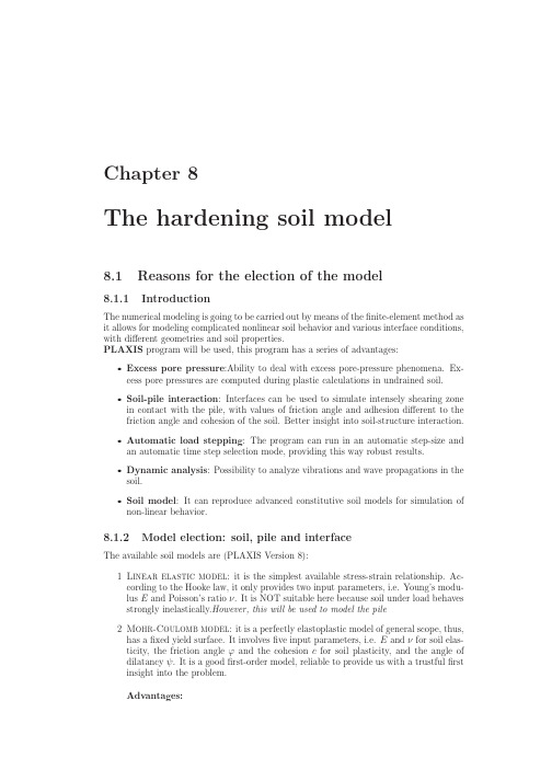
Chapter8The hardening soil model8.1Reasons for the election of the model8.1.1IntroductionThe numerical modeling is going to be carried out by means of thefinite-element method as it allows for modeling complicated nonlinear soil behavior and various interface conditions, with different geometries and soil properties.PLAXIS program will be used,this program has a series of advantages:•Excess pore pressure:Ability to deal with excess pore-pressure phenomena.Ex-cess pore pressures are computed during plastic calculations in undrained soil.•Soil-pile interaction:Interfaces can be used to simulate intensely shearing zone in contact with the pile,with values of friction angle and adhesion different to the friction angle and cohesion of the soil.Better insight into soil-structure interaction.•Automatic load stepping:The program can run in an automatic step-size and an automatic time step selection mode,providing this way robust results.•Dynamic analysis:Possibility to analyze vibrations and wave propagations in the soil.•Soil model:It can reproduce advanced constitutive soil models for simulation of non-linear behavior.8.1.2Model election:soil,pile and interfaceThe available soil models are(PLAXIS Version8):1Linear elastic model:it is the simplest available stress-strain relationship.Ac-cording to the Hooke law,it only provides two input parameters,i.e.Young’s modu-lus E and Poisson’s ratioν.It is NOT suitable here because soil under load behaves strongly inelastically.However,this will be used to model the pile2Mohr-Coulomb model:it is a perfectly elastoplastic model of general scope,thus, has afixed yield surface.It involvesfive input parameters,i.e.E andνfor soil elas-ticity,the friction angleϕand the cohesion c for soil plasticity,and the angle of dilatancyψ.It is a goodfirst-order model,reliable to provide us with a trustfulfirst insight into the problem.Advantages:86The hardening soil model•For each layer one estimates a constant average stiffness.Due to this constantstiffness computations are quite fast and give a goodfirst impression of theproblem.Shortcomings:•It can be too simpleInterfaces are normally modeled with this model3Jointed rock model:it is thought to model rock,NOT suitable here.4Hardening-soil model:it is an advanced hyperbolic soil model formulated inthe framework of hardening plasticity.The main difference with the Mohr-Coulombmodel is the stiffness approach.Here,the soil is described much more accurately byusing three different input stiffness:triaxial loading stiffness E50,triaxial unloadingstiffness E ur and the oedometer loading stiffness E oed.Apart from that,it accountsfor stress-dependency of the stiffness moduli,all stiffnesses increase with pressure(all three inputs relate to reference stress,100kP a).Advantages:•More accurate stiffness definition than the Mohr-Coulomb model(stress-dependentand stress-path dependent stiffness)•Takes into consideration soil dilatancy•The yield surface can expand due to plastic strainingShortcomings:•Higher computational costs•Does not include viscous effects•Does not include softening5Soft-soil-creep model:for soft soil(normally consolidated clays,silt or peat).NOT suitable here.6Soft soil model:for soft soil(normally consolidated clays,silt or peat).NOTsuitable here.For all the reasons presented above,Hardening soil model is the most appropriate to model the soil.More complex models can be implemented but then the user has to define them,andthis falls beyond the scope of this research.Finally,fig.(8.1)shows the conclusions.8.2Theoretical backgroundThe Hardening Soil model has been presented before as an hyperbolic model.Often hy-perbolic soil models have been used to describe the nonlinear behavior;this is also a suitable application in this research as sand usually behaves as a linear elastic material with shear modulus G for shear strains up to≈10−5,and afterward the stress-strain relationship is strongly non-linear(Lee,Salgado,1999).The background of this kind of models is the hyperbolic relationship between vertical strain and deviatoric stress in pri-mary triaxial loading.However,the Hardening-soil model is far better than the original8.2Theoretical background87Figure8.1:Chosen models for numerical analysis with PLAXIS hyperbolic model(Duncan and Chang,1970)as it uses theory of plasticity instead of the-ory of elasticity and because it includes soil dilatancy and a yield cap.In contrast to an elastic perfectly-plastic model like Mohr-Coulomb,now the yield surface is notfixed but can expand due to plastic straining.The main characteristics of the model are:•Stress dependent stiffness according to power law(defined by parameter m)•Plastic straining due to primary deviatoric stress(defined by parameter E ref50)•Plastic straining due to primary compression(defined by parameter E ref oed)•Elastic unloading/reloading(defined by parameter E ref ur,νur)•Failure according to the Mohr-Coulomb model(defined by parameters c,ϕ,ψ)In the Hardening Soil model,the associatedflow rule is defined as a relationship between rates of plastic shear strainγp and plastic volumetric strainǫp v;it has the linear form:ǫp v=sinψmγp(8.1) whereψm is the mobilized dilatancy angle,defined as:sinψm=sinϕm−sinϕcv1−sinϕm sinϕcv(8.2)withϕcv the critical state friction angle,constant for a certain material,independent of the density,andϕm the mobilized friction angle that can be calculated:sinϕm=σ′1−σ′3σ′1+σ′3−2c cosϕ(8.3)According to Rowe’s stress-dilatancy theory(1962),material contracts for small stress ratios(ϕm<ϕcv)and dilates for high stress-ratios(ϕm>ϕcv).At failure,the mobilized friction angle equals the failure one and:sinψ=sinϕ−sinϕcv1−sinϕsinϕcv(8.4)sinϕcv=sinϕ−sinψ1−sinϕsinψ(8.5)The parameters of the model are those of Mohr-Coulomb for the failure criteria(c,ϕ,ψ); in addition other parameters are introduced.88The hardening soil model•Secant stiffness in standard drained triaxial test:E ref 50,and then:E 50(σ)=E ref 50 c cos ϕ−σ′3c cos ϕ+p ref sin ϕ(8.6)•Tangent stiffness for primary oedometer loading:E ref oed •Power for stress-level dependency of stiffness:m •Unloading/reloading stiffness:E ref ur(default:E ref ur =3E ref 50),and then:E ur (σ)=E ref ur c cos ϕ−σ′3c cos ϕ+p ref sin ϕ (8.7)•Poisson’s ratio for unloading/reloading:νur (default:νur =0.2)•Reference stress for stiffness:p ref (default:p ref =100stress units)•K 0value for normal consolidation:K nc 0(default:K nc 0=1−sin ϕ)•Failure ratio:R f =q f /q a (default:R f =0.9)•Tensile strength:σtension (default:σtension =0)Also it defines the oedometer stiffness:E oed =E ref oed c cos ϕ−σ′1sin ϕc cos ϕ+p ref sin ϕ m (8.8)Note that the oedometer stiffness relates to oedometer testing,therefore to the compaction hardening part.On the other hand,E 50and E ur relate to triaxial testing and so to the friction hardening part.To explain the plastic volumetric strain in isotropic compression,a second yield surface closes the elastic region in the direction of the p-axis.While the shear yield surface is mainly controlled by the triaxial modulus,the oedometer modulus controls the cap yieldsurface.Figure 8.2:Cap surface of Hardening Soil model。
往复荷载下软土的边界面广义弹塑性模型
第21卷 第2期岩石力学与工程学报 21(2):210~2142002年2月 Chinese Journal of Rock Mechanics and Engineering Feb .,20022000年5月31日收到初稿,2000年6月27日收到修改稿。
* 国家自然科学基金重点资助项目(59738160)。
作者 周 健 简介:男,1957年生,工学博士,现任同济大学地下建筑与工程系教授、博士生导师,主要从事岩土工程教学与研究方面的工作。
往复荷载下软土的边界面广义弹塑性模型*周 健 孙吉主 吴世明(同济大学地下建筑与工程系 上海 200092)摘要 针对往复荷载作用下软土变形和孔压发展的特点,应用能模拟低应力水平下塑性变形的边界面模型,将其线弹性卸载过程改进为弹塑性,建立了软粘土的边界面广义弹塑性模型。
最后对该模型进行了试验验证,以表明其可靠性。
关键词 软土,边界面,本构关系,弹塑性分类号 TU 441,TU 434 文献标识码 A 文章编号 2000-6915(2002)02-0210-051 前 言实际工程中土受到复杂荷载作用的例子很多,如基坑开挖、隧道挖方和土坝蓄水、放空时的大幅度加载及卸载等等。
研究表明,对土材料来说,卸载、再加载及反向加载过程中同时伴随有弹性和塑性应变产生[1]。
显然经典的弹塑性模型不能对土体的这些力学特性予以充分的描述,因为经典塑性理论认为卸载与再加载时的响应均是弹性的,不产生塑性应变,这就需要建立新的塑性概念。
为此,出现了多种形态的弹塑性模型,如多重屈服面模型[2]、边界面模型[3]、内时理论模型[4]等。
对边界面本构模型的研究在国内起步较晚,但也取得了一定的成绩[5~8]。
为了较好地反映复杂荷载下软土的本构性质,本文在应用现有边界面模型[9]的基础上,试图对其卸载过程进行改进。
假设土体在卸荷过程中也同时发生弹性、塑性变形,因而加、卸载过程中都有一定的塑性变形产生,这种假设与软粘土几乎不存在一个纯弹性变形阶段的实际变形特性是一致的。
- 1、下载文档前请自行甄别文档内容的完整性,平台不提供额外的编辑、内容补充、找答案等附加服务。
- 2、"仅部分预览"的文档,不可在线预览部分如存在完整性等问题,可反馈申请退款(可完整预览的文档不适用该条件!)。
- 3、如文档侵犯您的权益,请联系客服反馈,我们会尽快为您处理(人工客服工作时间:9:00-18:30)。
Li,X.S.(2007).Ge´otechnique 57,No.5,423–435423Thermodynamics-based constitutive framework for unsaturated soils.2:A basic triaxial modelX.S.LI*Following the theoretical framework established in Part 1,a basic elastoplastic unsaturated soil model is formu-lated.The model is a combination of a soil skeleton model and an SWCC (soil-water characteristic curve)model.For simplicity,the model deals only with isotropic soils in triaxial compression space under a constant pore air pressure.The paper shows that the central element in the model that differentiates itself from a saturated model is its dual plastic hardening,which not only reflects the evolution of the internal structure of the soil skeleton but is also associated with the evolution of the solid–fluid interactive structure.For more flexible shear stress–strain responses,the non-associated flow rule (the alpha model)by Collins &Kelly,based on a thermody-namic analysis,is adopted.The present model introduces six new material constants,which can be calibrated following a systematic procedure.The model successfully simulates the multiple series laboratory tests reported by Sivakumar &Wheeler,including wetting,consolidation and shearing,on a compacted clay.KEYWORDS:constitutive relations;partial saturation;plasti-city;pore pressures;stress path;suctionUn mode`le e ´lastoplastique de sol non sature ´est formule ´sur la base du cadre the´orique de ´fini dans la partie 1.Il combine un mode`le de squelette solide et un mode `le de courbe caracte´ristique sol-eau (SWCC).Pour simplifier,ce mode`le ne traite que de sols isotropes dans un espace de compression triaxiale sous une pression d’air dans lespores constante.Cet article montre que l’e´le ´ment central du mode`le qui se distingue d’un mode `le sature ´est son double durcissement plastique,qui refle`te non seulement l’e ´volution de la structure interne du squelette solidemais correspond e´galement a `celle de la structure inter-active solide-fluide.On adopte la loi d’e´coulement non associe´e de Collins et Kelly (le mode `le alpha),base ´e sur une analyse thermodynamique,pour obtenir des re´ponses plus flexibles de contrainte-de´formation au cisaillement.Le mode`le pre ´sente ´ici introduit six nouvelles constantes de mate´riau,qui peuvent e ˆtre e ´talonne ´es suivant une proce´dure syste ´matique.Il simule avec succe `s les essais de se ´ries multiples rapporte ´s par Sivakumar et Wheeler,re´alise ´s en laboratoire sur une argile compacte ´e,incluant la mouillabilite´,la consolidation et le cisaillement.INTRODUCTIONA thermodynamics-based unsaturated soil modelling frame-work has been presented in the preceding companion paper (Li,2007),referred to as Part 1hereafter.The objective of the present paper (Part 2)is to demonstrate a specific model constructed in accordance with that framework.For effectively presenting the main idea,only a basic model is described in the sense that it deals only with isotropic soils in triaxial compression space with a constant pore air pressure.Extending the model to general 3D stress–strain space with a variable pore air pressure is straightforward;and modelling anisotropic features (includ-ing cyclic shearing)is a general,important,but separate issue beyond the scope of the present work,and therefore will not be addressed in this paper.In this model,because the pore air pressure is assumed to be constant,the behaviour of an unsaturated soil is described by two interrelated models:one for the solid skeleton,and the other for the pore fluids (referring to equations (88a)and (88b)in Part 1).As shown in Part 1,the former is constituted through specifically defined elastic moduli,plas-tic yielding,flow and hardening,and the latter is a model of soil-water characteristic curves (SWCC).All these model ingredients and their integration will be addressed in depth,supplemented with necessary references.The calibrationprocedure of model constants will also be presented in detail.To examine the performance of the model,the test results reported by Sivakumar &Wheeler (2000)and Wheeler &Sivakumar (2000)on compacted speswhite kaolin were simulated.A comparison between the simulated results and the test data shows that the model broadly captures the essential behaviour of the tested soil through all the stages,including wetting,consolidation and shearing,of the tests,indicating that the modelling framework proposed in Part 1and the specific model presented in Part 2(this paper)indeed have a sound basis.MODEL OF SOIL SKELETONIn triaxial compression space,the stress and strain tensors are reduced to two-component vectors~pq &'¼~óa þ2~ór ðÞ=3~óa À~ór &'(1a)andåv åq&'¼åa þ2år 2åa Àår ðÞ=3&'(1b)where åv and åq are the volumetric and deviatoric strainsrespectively,and ~pand q are the mean normal and deviato-ric stresses conjugate to d åv and d åq respectively in work done on the soil skeleton.In the definition,åa and år are theaxial and lateral strains respectively,and ~óa and ~ór are their corresponding stress conjugates.Manuscript received 11August 2005;revised manuscript accepted 25January 2007.Discussion on this paper closes on 3December 2007,for further details see p.ii.*Department of Civil Engineering,Hong Kong University of Science and Technology.Elastic relationsThe elastic response of the soil skeleton is described by the commonly used incremental relationsd~p¼K dåev ¼v0~pkdåev(2a)d q¼3G dåe q¼33K1À2íðÞ"#dåe q(2b) where K and G are the elastic bulk and shear moduli respectively;í(Poisson’s ratio)and k(a Cam clay para-meter)are two material constants;and v0is a reference specific volume at which the volumetric strainåv¼0.Note that the shear modulus so defined depends on the mean normal stress~p,making equation(2b)hypoelastic:this means that the relationship given by equation(2b)is not exactly elastic,in the sense that recovery of the devia-toric stress upon an arbitrary closed cycle of strainåe q is not guaranteed.The impact of this effect on the overall stress–strain response,however,is considered negligible,because of the dominance of plastic deformation.In other words,in this model the elastic and plastic deviatoric strain increments aredenoted as dåeq and dåpqinstead of general infinitesimalsäåeqandäåp q(referring to the notation in Part1)only in an approximate sense.On the other hand,equation(2a)is an integrable equation,which makes the relationship between~pandåev exactly elastic(path independent).Although this factis widely known from study of the Cam clay models,it is worth reiterating that,because of this exactly elastic relation-ship,the effect of the plastic volumetric strainåp v is guaran-teed to be path independent,and consequently it can be treated as a perfect internal state variable in formulating the hardening laws.In the present model,the internal structure of the soil skeleton,H9s,is uniquely characterised byåp v. Yield function and plasticflowIn the triaxial space,the dissipative equilibrium equation (equation(37)in Part1)is reduced top D Dþq DÀv s¼~pÀpÆðÞDþqÀqÆðÞÀr s iæs i¼0(3)where p D and q D are the dissipative stresses;D¼dåp v=dåp q is the dilatancy such that the direction of the plastic strain increment m is equal to f D1g T and the loading index L s is equal to dåp q;and pÆand qÆare the back mean normal and deviatoric stresses.In this model,as the material is treated as isotropic,the yield function must be unbiased with respect to all three principal stress axes,and accordingly the deviatoric back stress qÆmust vanish identically,resulting in q D q.By setting q D¼q,takingåp v andåp q as two internal variables,and then following the idea of Collins&Kelly (2002)concerning a non-associatedflow rule(the alpha model),the above equation is converted into the more concrete formp D Dþq¼ð0DffiffiffiffiffiffiffiffiffiffiffiffiffiffiffiffiffiffiffiffiffiffiffiffiD2þM2R2p!|fflfflfflfflfflfflfflfflfflfflfflffl{zfflfflfflfflfflfflfflfflfflfflfflffl}æs1D|{z}r s1þð0M2R2ffiffiffiffiffiffiffiffiffiffiffiffiffiffiffiffiffiffiffiffiffiffiffiffiD2þM2R2p"#|fflfflfflfflfflfflfflfflfflfflfflfflffl{zfflfflfflfflfflfflfflfflfflfflfflfflffl}æs21|{z}r s2 |fflfflfflfflfflfflfflfflfflfflfflfflfflfflfflfflfflfflfflfflfflfflfflfflfflfflfflfflfflfflfflfflfflfflfflfflfflfflfflffl{zfflfflfflfflfflfflfflfflfflfflfflfflfflfflfflfflfflfflfflfflfflfflfflfflfflfflfflfflfflfflfflfflfflfflfflfflfflfflfflffl}v s(4)where M is the well-known critical state stress ratio,andð0 and R are state functions.Equation(4)indicatesp D¼ð0DffiffiffiffiffiffiffiffiffiffiffiffiffiffiffiffiffiffiffiffiffiffiffiffiD2þM2R2p(5a) andqMR¼ð0MRffiffiffiffiffiffiffiffiffiffiffiffiffiffiffiffiffiffiffiffiffiffiffiffiD2þM2R2p(5b)Adding the squares of the above two equations together results in the yield function in the dissipative stress space,f s¼M2R2p2Dþq2ÀM2R2ð20¼0(6)Equation(6)represents an ellipse in dissipative stress space. By denoting the values of~p on the yield surface intercepting the hydrostatic axis(q¼0)as p b and p0+p b respectively, one hasð0¼p0=2¼pÆÀp b(7) The dilatancy is then obtained by imposing the normality rule in the dissipative stress space:D¼@f s=@p D@f s=@q¼M2R2p Dq¼M2R2~pÀpÆðÞq(8)where R is given,based on the original proposition of Collins&Kelly(2002),asR¼Æþ1ÀÆðÞp Dþð0ð0¼Æþ1ÀÆðÞ~pÀpÆþð0ð0(9) in whichÆis a material constant.In the present model,ð0¼ð0(åp v,ns,S r)and pƼpÆ(åp v, ns,S r).Such functional dependences make the thermody-namic forcesæs1andæs2depend not only on the internal state variable of the soil skeletonåp v but also on thefluid state variables ns and S r(referring to equations(16)and(17)in Part1).Combining equations(6),(7)and(9)transforms the yield function into the true stress space,reading asf s¼f s~p,q,p0åp v,ns,S rÀÁ,p båp v,ns,S rÀÁÂüf s€p,q,p0ðÞ¼M241ÀÆðÞ2€p4p2À41À3Æþ2Æ2ðÞ€p3p0ÀÆ4À5ÆðÞ€p2ÀÆ2€p p0!þq2¼0(10)where€p¼~pÀp b(11) is the shifted mean normal stress.Fig.1shows the yield function plotted in true~pÀq stress space.It can be seen that p b is the back mean normal stress(referring to equation (78)in Part1)that controls the position of the yield surface in the true stress space,and p0characterises the size of the yield surface.Note that becauseð0¼ð0(åp v,ns,S r),p b and p0are,in general,both functions of the state variablesåp v,ns and S r.The condition of consistency of the yield function reads asd f s¼@f s@~pd~pþ@f s@qd qþ@f s@p0d p0þ@f s@p bd p b¼@f s@€pd€pþ@f s@qd qþ@f s@p0d p0¼0(12)424LIwith the partial derivatives given by @f s @~p ¼À@f s @p b ¼@f s@€p¼M2"161ÀÆðÞ2€p 3p 20À121À3Æþ2Æ2ðÞ€p 2p 0À2Æ4À5ÆðÞ€p ÀÆ2p 0#(13a)@f s @q ¼@f s@q ¼2q (13b)@f s @p 0¼@f s@p 0¼M 2À81ÀÆðÞ2€p 4p 30þ41À3Æþ2Æ2ðÞ€p3p 20ÀÆ2€p "#(13c)It can be seen that ì¼{@f s /@~p @f s /@q }T is in general notco-directional with m ¼{D 1}T ,indicating that a non-associative plastic flow is materialised.As demonstrated by Collins &Kelly (2002),the above yield function (with p b ¼0)is reduced to the modified Cam clay yield function when the parameter Ƽ1,and only in this special case is the associated flow rule resumed.It should be remarked that the yield function,as well as the corresponding flow rule presented above,was originally proposed by Collins &Kelly (2002)based on their thermo-dynamic framework for saturated soils.The adoption of this yield function is based on the consideration that its non-associated flow rule offers more flexibility in modelling shear stress–strain behaviour by adding only one more material constant,as compared with the modified Cam clay yield function.However,the latter,as well as many other existing yield functions,can also be adopted.Hardening and plastic moduliThe present model includes both isotropic hardening and kinematic hardening,characterised by the internal state vari-ables p 0and p b respectively.It is noted that in both the Cam clay and the Collins &Kelly models,p b 0,and p 0is assumed to depend only on the plastic volumetric strain.This is valid only for saturated soils,as it involves no impact of unsaturation.In the present unsaturated soil mod-el,as attention was called to earlier,the two hardeningvariables p b and p 0depend not only on åp v but also on ns and S r ,the state variables of the pore fluids.Such depen-dences are consistent with the theoretical framework pre-sented in the companion paper (Part 1),and are vital for a proper modelling of essential unsaturated soil behaviour.The hardening response is investigated here through iso-tropic compression.Fig.2shows a simple mechanism of aparticle sliding under macroscopically isotropic stress ~p.It is assumed that an irreversible change in volume is attrib-uted mainly to particle sliding (although the macroscopic shear strain may be zero),which repacks the particle assem-blage into a different density state.During isotropic com-pression,both the normal and shear forces at particlecontacts are associated with ~p.When ~p Àp b is less than a threshold p 0,the contact shear force is,on average,less than the product of the contact normal force and the coefficient of friction between particle minerals,such that sliding is notmaterialised.When ~pÀp b ¼p 0,the resultant normal force times the coefficient of friction Øis equal to the resultant shear force,as illustrated in Fig.2.This is the macroscopic yield condition.By scaling the resultant shear force to Øp 0,the resulting normal force is equal to p 0,which is a state function that can be written in the formp 0åp v ,ns ,S r ÀÁ¼p ååp v ÀÁþp ìåp v ,ns ,S r ÀÁ(14)where p åis a parameter of the soil skeleton solely related to its internal structure (H 9s ),and p ìreflects the impact of the solid–fluid interaction (H 0s ).Note that for a soil in saturated or dry states H 0s disappears,and so does p ì(to be consistent with saturated models,in saturated or dry states the back-pressure p b ¼0as well).This indicates that p åis simply the yield confining pressure for the soil in saturated or dry states,given by the well-known empirical observation (Schofield &Wroth,1968)p ååp v ÀÁ¼eN Àv p ºÀk ¼e N Àv p 0þv 0åp v ºÀk (15)where º,k and N are the well-known Cam clay constants,denoting the slopes of the normal consolidation line and therebound lines in the v Àln ~pplane and the value of the specific volume on the isotropic consolidation line at ~p¼1(note that in saturated states p b vanishes,so it plays no role)respectively;and v p and v p 0are the plastic parts of the specific volume and its initial value respectively.As shown in the above equation,p åis uniquely related to v p ,meaning that p åis an internal state variable of the soil skeleton.That is,p åevolves only when the soil skeleton experiences an internal structural change (an irrecoverable volume change).In this basic model,it is further assumed that p å(or,equivalently,v p or åp v )is the only internal state variable of the soilskeleton.1020304050p : kPa: k P aq ~Fig.1.Yield surface in ~p2qplane p ns S p p ns Sp p p ns S p ns S 0p v r p v pv r p vp vrbp vr(,,)()(,,)()(,,)(,,)εεεεεεϭϩϭϩϩεµεµ~Fig.2.Sliding block model for yielding under isotropic stressconditionTHERMODYNAMICS-BASED CONSTITUTIVE FRAMEWORK FOR UNSATURATED SOILS 2425On the other hand,p ìcharacterises the impact of solid–fluid interaction (meniscus effects)on the soil skeleton,which is related not only to åp v but also to the fluid state variables ns and S r .This means that p ì,and consequently the size of the yield surface (p 0),may change even if the internal structure of the soil skeleton remains unchanged.This is the case where äH 9s ¼0but äH s ¼0(referring to equation (43)in Part 1).For example,during wetting,as suction becomes smaller,p ìis reduced,as is p 0.However,itis entirely possible that ~pÀp b is smaller than p 0such that the soil skeleton still remains in elastic states until ~pÀp b ¼p 0.As p ìcharacterises the impact of meniscus effects on the soil skeleton,it is zero when ns ¼0(soil is saturated)or S r ¼0(soil is dry).For convenience,an intermediate para-meter ì(åp v ,ns ,S r )>1is introduced,with ì¼1for ns ¼0or S r ¼0,such that p ì¼1Àr ðÞìc À1ðÞp å(16a)orp 0¼p ìþp å¼ìc Àr ìc À1ðÞ½ p å(16b)where r and c are material constants.In this model,ìis given by the following empirical relation (other specific functions may be proposed when more test data become available):ì¼ìåp v ,ns ,S r ÀÁ¼1þap 1Àb atm nsS r ðÞb p å¼1þap 1Àbatm nsS r ðÞb ev pÀv 0åp v ÀN ºÀk(17)where a and b are two additional material constants,and p atm is the atmospheric pressure,serving as a reference to make the material constants dimensionless.The parameters a ,b ,c and r are all the material constants added to conven-tional saturated model constants to characterise the behav-iour of the soil skeleton.The calibration procedure of these new constants will be presented later.It can be seen that equation (17)satisfies the constraint that ì¼1for ns ¼0or S r ¼0;and ìtends toward unity as soil becomes denser,reflecting the general trend that soil becomes more stable (less affected by solid–fluid interaction)when it has a denser structure (Vicol,1990).As p ìand the back mean normal stress p b both originate from meniscus effects,they are homogeneously related.As a first approximation,p b is assumed to be proportional to p ì,asp b ¼r1Àr p ì¼r ìc À1ðÞp å(18)such that the isotropic yield stress is given by the simple relation~p¼p 0þp b ¼p åìc (19)It is interesting to note that both ~p¼þsS r and p 0+p b are functions of sS r ,with ~p<p 0þp b always.If initially ~p,p 0þp b (say,immediately after compaction),when wet-ting proceeds under a constant net pressure p ,sS r decreases,and so do ~pand p 0+p b .If the decreasing rate of p 0+p b is greater than that of ~p,at a particular value of sS r ,~p may be equal to p 0+p b ,signalling the onset of plastic yielding.Any further decrease of sS r after that instant will be associated with a permanent volume reduction.This is the case of collapse.As illustrated in Fig.3,collapse may occur only when p is greater than the initial p å,indicating that,during wetting,collapse is likely to occur if the applied pressure (p )is high and/or the material is loose (p åis low).The evolution of the isotropic hardening state variable p 0is given by differentiating equation (16b),with ìreplacedby equation (17),as follows:d p 0¼1Àr ðÞìc þr ÂÃd p åþc 1Àr ðÞp åìc À1d ì¼1Àr ðÞìc þr ÂÃ@p å@åp v þc 1Àr ðÞp åìc À1@ì@åp v &'d åp vþc 1Àr ðÞp åìc À1@ì@S r þ@ì@ns ðÞ@ns ðÞ@S r!d S r ¼v 0p 0þp b ðÞºÀk p 00b À1Àr ðÞc ìÀ1ðÞì!d åp vþ1Àr ðÞbc p 0þp b ðÞìÀ1ðÞns þS r ÇðÞnsS r ìd S r(20)and the evolution of the kinematic hardening state variable p b is given by differentiating equation (18),with ìreplaced by equation (17),asd p b ¼r ìc À1ðÞd p åþcr ìc À1p åd ì¼v 0p 0þp b ðÞºÀkp b p 0þp b Àr c ìÀ1ðÞì !d åp vþrbc p 0þp b ðÞìÀ1ðÞns þS r ÇðÞnsS r ìd S r(21)where the relations given in equations (15)and (17)have been invoked.In the above equation,Ǽ@(ns )=@S r is to be determined by a separate SWCC model (referring to equa-tion (69)in Part 1),which in the present work features the hysteretic response of the scanning curves (see next section)so that Çis hydraulic path dependent.By combining equations (12),(20)and (21),invoking thedefinition d åp v ¼D d åpq ¼D h L s i ,and then referring to equa-tion (45)in Part 1,one obtains the plastic moduliK 9p ¼v 0p 0þp b ðÞD ºÀk (@f s @€p p b p 0þp b Àrc ìÀ1ðÞì!À@f s @p 0p 0p 0þp b À1Àr ðÞc ìÀ1ðÞì !)(22)andInitial p sS rFig.3.Illustration of evolution of p 0+p b during wetting426LIK 0p¼@f s @€p r À@f s@p 01Àr ðÞ"#bc p 0þp b ðÞìÀ1ðÞns þS r ÇðÞnsS r !(23)where the partial derivatives @f s =@€p and @f s =@p 0havebeen given in equations (13a)and (13c),and the dilatancy Dhas been given by equation (8),in combination with equa-tions (7)and (9).Note that when yielding takes place under isotropic stress conditions,€p ¼p 0so that @f s =@€p ¼À@f s =@p 0(refer to equations (13a)and 13(b));and,accord-ingly,the roles of r in equations (22)and (23)are elimi-nated,which means that the material constant r plays no part in isotropic consolidation and/or isotropic wetting/dry-ing.Note also that as Çis wetting/drying path dependent,K 0p is wetting/drying path dependent,too,which means that the soil deformation induced by hydraulic actions depends on the history of the hydraulic process.MODEL OF HYDRAULIC RESPONSEThe bounding surface SWCC model proposed by Li (2005)based on phenomenological observations on s –S r scanning curves is used in the present study with a minor modification:that is,the soil-water characteristic curves are expressed as relations between ns and S r ,rather than be-tween s and S r ,because ns and S r are conjugate in volume-specific work,as shown in equation (19b),Part 1.The model assumes two primary soil-water characteristic curves for a given soil.One is f d (ns ,S r )¼0for primary drying (presumably starting from a full saturation state)and the other is f w (ns ,S r )¼0for primary wetting (presumably starting from a completely dry state),where s is called the image suction,referred to as the values of suction on the primary curves.These two curves serve as the bounds of all scanning curves.In addition,a weighted back suction (referring to equation (59)in Part 1)is also defined,which is the product of porosity n and the value of suction at which the last reversal of the hydraulic process from wetting to drying,or vice versa,took place.Because the weighted back suction changes discontinuously (only when the hy-draulic process changes the direction),the value of is piecewise (within each scanning curve)constant.In the model,the wetting/drying state is specified by the degree of saturation S r and three weighted suction values,ns ,and ns ,with representing the impact of the wetting/drying history.The relations among these state variables and their increments are illustrated in Fig.4.Refer to Li (2005)for more details (with slightly different notations:and d ¼Æand â,respectively,in Li,2005).The general incremental relationship among ns ,S r and åhas been given by equation (69)in Part 1.In the present model,partially because of lack of systematic experimental results,the relation is simplified by assuming ˛¼0.That is,the impact of solid–fluid interaction on SWCC is consid-ered to be negligible.Therefore d ns ðÞ¼H 9p M f H 9p þsgn äS p rÀÁ|fflfflfflfflfflfflfflfflfflfflfflfflfflfflffl{zfflfflfflfflfflfflfflfflfflfflfflfflfflfflffl}Çd S r ¼Çd S r (24)Following Li (2005),the stiffness Çis given byǼj ln ns =âÀÁj dH j ln ns =âÀÁj d þj ln ns =âÀÁj d H À1ðÞ"#s s d ns ðÞd S r (25)where H and d are two model parameters,which can be either constants or state functions.In the present work they are both treated as constants for simplicity.The parameter d controls the ‘fatness’of the hysteresis loops formed by the scanning curves.It can be seen from equations (24)and (25)that,when a scanning curve starts right after a change in wetting/drying direction,ns ¼â,and the ratio d ln (ns )=d ln (ns )¼H ,which controls the initial slope of the scan-ning curve;and as ns moves on its way towards ns ,the slope of the curve varies smoothly,and when ns gets close to ns ,d ln (ns )=d S r %d ln (ns )=d S r ,indicating that a scan-ning curve is an asymptote of its respective primary SWCC.The model described above can be used in conjunction with any propositions for the primary wetting and drying curves.In this study,a version of the SWCC equation proposed by Fredlund &Xing (1994)is used,which is S r ¼1ln exp (1)þns kp atml "#()m(26)where k ,l and m are curve-fitting parameters.In this model,there are two sets of such constants,k d ,l d ,m d and k w ,l w ,m w for the primary drying and wetting curves respectively.STIFFNESS MATRIXAs stated earlier,for simplicity,the pore air pressure in the present model has been assumed as a constant (pore air spaces connect to a constant pressure source,say,the atmo-spheric pressure;and loading is sufficiently slow),so that equation (88)in Part 1consists of only the first two simul-taneous equations,which in the triaxial space can be written asd ~pd q d ns ðÞ8<:9=;¼¸11¸12—1¸21¸22—20Ç2435d åv d åqd S r8<:9=;(27)where ˛has already been set at 0.In the above equation,the coefficients ¸ij and —i are the components of the stiffness matrices ¸and —given by equations (53)and (54)of Part 1,which in the triaxial space are writtenas0·20·40·60·81·0ns : kPaS rFig.4.Illustration of bounding surface SWCC modelTHERMODYNAMICS-BASED CONSTITUTIVE FRAMEWORK FOR UNSATURATED SOILS 2427。