大涡模拟
二维大涡模拟步骤

二维大涡模拟步骤二维大涡模拟(Large Eddy Simulation, LES)是一种基于Navier-Stokes方程的数值模拟方法,用于研究流体力学中的湍流现象。
它是在雷诺平均湍流模拟(Reynolds-averaged Navier-Stokes, RANS)的基础上发展起来的一种高精度模拟方法。
下面将详细介绍二维大涡模拟的步骤。
1.定义几何模型:首先需要定义流动的几何模型,包括计算域的形状和尺寸以及边界条件。
对于二维大涡模拟,计算域通常是一个二维平面。
边界条件可以是速度入口、压力出口或壁面,这些条件将在模拟过程中保持不变。
2.网格划分:将计算域划分为离散的小单元,形成计算网格。
网格的划分需要根据流动的复杂程度和几何形状进行调整,以确保模拟结果的精度。
在二维大涡模拟中,通常采用结构化网格或非结构化网格。
3.初始化:在模拟开始之前,需要对流体的初始状态进行初始化。
这包括设置流体的初始速度场和压力场。
对于具体的问题,初始条件可以使用已有的实验数据或理论结果进行设定。
4. 求解Navier-Stokes方程:二维大涡模拟是基于Navier-Stokes方程进行求解的。
该方程描述了流体速度和压力随时间和位置的变化关系。
通过用有限体积或有限差分等数值方法离散化Navier-Stokes方程,可以得到一个离散的代数方程组。
5.大涡模拟模型:在LES中,大尺度涡旋由数值模拟解决,而小尺度涡旋则采用传统的湍流模型进行处理。
LES使用了一个滤波器来将流动场分解为大尺度和小尺度的成分。
对于大尺度成分,可以通过直接数值模拟来解决;而对于小尺度成分,可以采用传统的湍流模型,如k-ε模型或k-ω模型。
在大涡模拟模型中,需要确定滤波器的类型和大小。
6. 时间步进:通过将时间离散化为一系列离散时间步长,可以在每个时间步长内求解Navier-Stokes方程。
时间步长的选择要满足稳定性和精度的要求。
通常可以通过在计算过程中进行数值稳定性和收敛性分析来确定最佳的时间步长。
大气表面层气-固颗粒两相流的大涡模拟

大气表面层气-固颗粒两相流的大涡模拟大气表面层气-固颗粒两相流的大涡模拟引言:随着科技的不断发展,气-固两相流模拟已经成为研究气候变化、空气质量等大气问题的一种重要方法。
在大气表面层,气-固两相流的运动现象非常复杂,需要借助先进的数值模拟方法来研究。
本文将介绍大涡模拟这一常用的方法,并探讨其在大气表面层气-固颗粒两相流研究中的应用。
一、气-固颗粒两相流的特点大气表面层气-固颗粒两相流是一个复杂的多相流现象,涉及气体与固体颗粒之间的相互作用。
在大气表面层,气体一方面受到地面的辐射、热对流等作用,另一方面还要承受固体颗粒的碰撞、输送等作用。
而固体颗粒则在气流的冲击下发生分散、聚集等运动。
二、大涡模拟方法大涡模拟是一种求解大涡模型的数值模拟方法,适用于研究粗粒度涡动结构。
它以较大尺度上的涡旋为研究对象,通过模拟其演化过程来探究流体的物理行为。
与传统的雷诺平均纳维-斯托克斯方程相比,大涡模拟能够更好地模拟湍流流场的结构和特性。
三、大涡模拟在气-固颗粒两相流中的应用在大气表面层气-固颗粒两相流研究中,大涡模拟方法得到了广泛的应用。
首先,大涡模拟能够有效地模拟气流中的湍流结构,从而研究气-固颗粒在气流中的运动和输运行为。
其次,大涡模拟还可以用于研究气-固颗粒之间的相互作用,包括颗粒的沉降、聚集、碰撞等过程。
最后,大涡模拟还可以模拟大气表面层中的气-固颗粒的输运过程,对于研究颗粒的输送距离、浓度分布等具有重要意义。
四、案例研究以研究大气表面层的颗粒污染物扩散为例,利用大涡模拟方法可以模拟大气湍流结构中的颗粒运动情况。
首先,通过模拟湍流气流的运动,得到湍流结构的分布和变化规律。
然后,在此基础上引入颗粒模型,模拟颗粒在湍流气流中的输运行为。
通过对模拟结果的分析,可以得到颗粒的浓度分布、输送距离以及颗粒与气流之间的相互作用等重要信息。
结论:大涡模拟方法在大气表面层气-固颗粒两相流研究中具有广阔的应用前景。
它能够很好地模拟气流中湍流结构的演化过程,并揭示气-固颗粒之间复杂的相互作用。
大涡模型参数
大涡模型参数
大涡模型(LES)是一种计算流体力学技术,它对大尺度湍流结构进
行直接模拟,而对小尺度湍流结构进行模型化处理。
在模拟过程中,LES
需要设定很多参数,下面是一些常见的发挥作用的参数:
1.网格大小:LES需要对流场进行网格化,在实际应用中,网格大小
对计算结果的准确性和计算时间都有很大影响。
2.积分时间步长:LES需要对计算时间进行离散化,以便于计算机进
行运算,积分时间步长越小,计算结果越精确,但计算时间也会增加。
3.物理模型:LES需要对流场中的运动状态、物理现象进行模型化处理,包括雷诺应力模型、湍流能谱模型等。
4.物理参数:LES需要设定一些物理参数,如涡粘系数、湍流能谱、
湍流弛豫时间等。
5.数值参数:LES需要设定一些数值参数,如守恒方程数值离散化方案、格式、求解方法等。
6.起始条件:LES需要设定流场的起始条件,包括流速、压力、温度、密度等。
以上参数均需要经过一定的试验和实践,才能得出最佳参数组合,以
实现LES的最佳计算效果。
切变对流和热力对流的大涡模拟实验

切变对流和热力对流的大涡模拟实验大气边界层通常是指大气的最低部分受地面影响的一层,平均厚度约为地面以上1km范围[1]。
大气边界层内空气的运动的根本特点是湍流。
人们对湍流的研究已有近百年的历史,1839年,G.汉根在实验中首次观察到由层流到湍流的转变。
1883年,O.雷诺又在圆管水流实验中找出了层流过渡到湍流的条件。
在理论研究方面,1895年雷诺曾把瞬时风速分解为平均风速和叠加在上面的湍流脉动速度两部分,得到湍流运动方程组(雷诺方程),提出湍流粘性力(雷诺应力)的概念。
1925年,L.普朗特在此基础上提出了混合长度的概念,得出边界层内风速随高度变化的规律,即在对数坐标中风速随高度增加而呈线性增长[2]。
在大气边界层中,此结果被许多实验所证实。
1915年,G.I.泰勒提出了研究大气湍流微结构的统计理论。
1920年,L.F.理查孙研究了大气温度分布对湍流的影响,研究结果表明温度的铅直分布对大气湍流的影响,取决于大气静力稳定度。
一般可用理查孙数(R)判别稳定度对湍流的作用。
1941年,A.H.科尔莫戈罗夫又提出了局地各向同性理论,以上这些理论,合理地解释了湍流中的微结构。
当地表受热形成热泡或气流受到障碍物的阻挡发生扰流都能形成边界层湍流,当这种湍流进一步发展,就会形成对流。
一般把边界层对流分成两种形式:切变对流和热力对流。
边界层中切变对流其实主要与风切变有关,而风切变是气流的运动速度大小和方向突然发生变化,它可以出现在垂直方向上和水平方向上。
近年来,边界层切变对流的研究受到越来越多的重视,例如受风切变影响较大的边界层顶夹卷过程是接影响对流边界层的发展, 并且对对流边界层与自由大气之间物质和能量交换有重要作用。
Hoxit L R.的研究表明,夹卷过程能够显著影响着边界层中的风廓线和湿度垂直分布, 对于数值天气预报模式和空气污染模式也是非常重要的一个过程[3-5]。
以往对夹卷层的研究主要针对纯浮力驱动的对流边界层,对夹卷过程的参数化相对比较简单。
大涡模拟的FLUENT算例2D
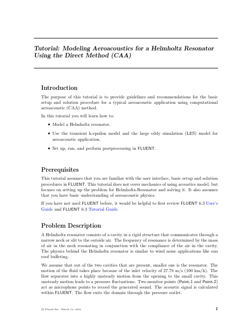
Tutorial:Modeling Aeroacoustics for a Helmholtz Resonator Using the Direct Method(CAA)IntroductionThe purpose of this tutorial is to provide guidelines and recommendations for the basic setup and solution procedure for a typical aeroacoustic application using computational aeroacoustic(CAA)method.In this tutorial you will learn how to:•Model a Helmholtz resonator.•Use the transient k-epsilon model and the large eddy simulation(LES)model foraeroacoustic application.•Set up,run,and perform postprocessing in FLUENT.PrerequisitesThis tutorial assumes that you are familiar with the user interface,basic setup and solution procedures in FLUENT.This tutorial does not cover mechanics of using acoustics model,but focuses on setting up the problem for Helmholtz-Resonator and solving it.It also assumes that you have basic understanding of aeroacoustic physics.If you have not used FLUENT before,it would be helpful tofirst review FLUENT6.3User’s Guide and FLUENT6.3Tutorial Guide.Problem DescriptionA Helmholtz resonator consists of a cavity in a rigid structure that communicates through anarrow neck or slit to the outside air.The frequency of resonance is determined by the mass of air in the neck resonating in conjunction with the compliance of the air in the cavity.The physics behind the Helmholtz resonator is similar to wind noise applications like sun roof buffeting.We assume that out of the two cavities that are present,smaller one is the resonator.The motion of thefluid takes place because of the inlet velocity of27.78m/s(100km/h).The flow separates into a highly unsteady motion from the opening to the small cavity.This unsteady motion leads to a pressurefluctuations.Two monitor points(Point-1and Point-2) act as microphone points to record the generated sound.The acoustic signal is calculated within FLUENT.Theflow exits the domain through the pressure outlet.Modeling Aeroacoustics for a Helmholtz Resonator Using the Direct Method(CAA) Preparation1.Copy thefiles steady.cas.gz,steady.dat.gz,execute-by-name.scm,stptmstp4.scm,ti-to-scm-jos.scm and stptmstp.txt into your working directory.2.Start the2D double precision(2ddp)version of FLUENT.Setup and SolutionStep1:Grid1.Read the initial case and datafiles for steady-state(steady.cas.gz and steady.dat.gz).File−→Read−→Case&Data...Ignore the warning that is displayed in the FLUENT console while reading thesefiles.2.Keep default scale for the grid.Grid−→Scale...3.Display the grid and observe the locations of the two monitor points,Point-1andPoint-2(Figure1).Figure1:Graphics Display of the Grid4.Display and observe the contours of static pressure(Figure2)and velocity magnitude(Figure3)for the initial steady-state solution.Display−→Contours..Modeling Aeroacoustics for a Helmholtz Resonator Using the Direct Method(CAA)Figure2:Contours of Static Pressure(Steady State)Figure3:Contours of Velocity Magnitude(Steady State)Modeling Aeroacoustics for a Helmholtz Resonator Using the Direct Method(CAA) Step2:Models1.Select unsteady solver.Define−→Models−→Solver...(a)Select Unsteady in the Time list.(b)Select2nd-order-implicit in the Unsteady formulation list.(c)Retain the default settings for other parameters.(d)Click OK to close the Solver panel.2.Define the viscous model.Define−→Models−→Viscous...(a)Select Non-Equilibrium Wall Functions in the Near-Wall Treatment list.(b)Retain the default settigns for other parameters.(c)Click OK to close the Viscous Model panel.Near-Wall Treatment predicts good separation and re-attachment points.Step3:MaterialsDefine−→Materials...1.Select ideal-gas from the Density drop-down list.2.Retain the default values for other parameters.3.Click Change/Create and close the Materials panel.Ideal gas law is good in predicting the small changes in the pressure.Step4:Solution1.Monitor the static pressure on point-1and point-2.Solve−→Monitors−→Surface...(a)Enter2for the Surface Monitors.(b)Enable Plot and Print options for monitor-1and monitor-2.(c)Select Time Step from the When list.(d)Click Define...for monitor-1to open Define Surface Monitor panel.Modeling Aeroacoustics for a Helmholtz Resonator Using the Direct Method(CAA)i.Select Vertex Average from the Report Type drop-down list.ii.Select Flow Time from the X Axis drop-down list.iii.Enter1for Plot Window.iv.Select point-1from the Surfaces selection list.(e)Similarly,specify the surface monitor parameters for point-2.2.Start the calculations using the following settings.Solve−→Iterate...(a)Enter3e-04s for Time Step Size.The expected time step size for this problem is of the size of about1/10th of thetime period.The time period depends on the frequency(f)which is calculatedusing the following equation:f=c2πSV[L+π2.D h2]where,c=Speed of soundS=Area of the orifice of the resonatorV=Volume of the resonatorL=Length of the connection between the resonator and the freeflow areaD h=Hydraulic diameter of the orificeFor this geometry,the estimated frequency is about120Hz.(b)Enter250for the Number of Time Steps.(c)Enter50for Max Iterations per Time Step.(d)Click Apply.Modeling Aeroacoustics for a Helmholtz Resonator Using the Direct Method(CAA)(e)Read the schemefile(stptmstp4.scm).File−→Read−→Scheme...Thisfile activates a alternative convergence criteria.For acoustic simulationswith CAA it is obligatory that the pressure is completely converged at the recieverposition.FLUENT compares the monitor quantities within the last n-defined it-erations to judge if the deviation is smaller than a y-defined deviation.(f)Specify the number of previous iterations from which monitor values of eachquantity used are saved and compared to the current(latest)value(include theparanthesis):(set!stptmstp-n5)(g)Specify the relative(the smaller of two values in any comparison)differenceby which any of the older monitor values(for a selected monitor qauntity)maydiffer from the newest value:(set!stptmstp-maxrelchng1.e-02)(h)Define the execute commands.Solve−→Execute Commandsi.Enter(stptmstp-resetvalues)for thefirst command and select Time Stepfrom the drop-down list.ii.Enter(stptmstp-chckcnvrg"/report/surface-integrals vertex-avg point-1 ()pressure")and select Iteration from the drop-down list.iii.Click OK.(i)Click Iterate to start the calculations.The iterations will take a long time to complete.You can skip this simulation af-ter few time steps and read thefiles(transient.cas.gz and transient.dat.gz)provided with this tutorial.Thesefiles contain the data for theflow time of0.22seconds.As seen in Figures4and5,no pressurefluctuations are present at thisstage.The oscillations of the static pressure at both monitor points has reacheda constant value.The RANS-simulation is a good starting point for Large Eddy Simulation.Ifyou choose to use the steady solution as initial condition for LES,use the TUIcommand/solve/initialize/init-instantaneous-vel provides to get a more realisticinstantaneous velocityfield.The usage of LES for acoustic simulations is obliga-tory.The next two pictures compare the static pressure obtained with RANS andLarge Eddy Simulation for a complete simulation until0.525seconds.Obviously,the k-epsilon model underpredicts the strong pressure oscillation after reachinga dynamically steady state(>0.3s)due to its dissipative character.Under-predicted pressure oscillations lead to underpredicted sound pressure level whichmeans the acoustic noise is more gentle.Modeling Aeroacoustics for a Helmholtz Resonator Using the Direct Method(CAA)Figure4:Convergence History of Static Pressure on Point-1(Transient)Figure5:Convergence History of Static Pressure on Point-2(Transient)Modeling Aeroacoustics for a Helmholtz Resonator Using the Direct Method(CAA) Step5:Enable Large Eddy Simulation1.Enter the following TUI command in the FLUENT console:(rpsetvar’les-2d?#t)2.Enable large eddy simulation effects.The k-epsilon model cannot resolve very small pressurefluctuations for aeroacousticdue to its dissipative e Large Eddy Simulation to overcome this problem.Define−→Models−→Viscous...(a)Enable Large Eddy Simulation(LES)in the Model list.(b)Enable WALE in the Subgrid-Scale Model list.(c)Click OK to close the Viscous Model panel.An Information panel will appear,warning about bounded central-deferencing be-ing default for momentum with LES/DES.Modeling Aeroacoustics for a Helmholtz Resonator Using the Direct Method(CAA)(d)Click OK to close the Information panel.3.Retain default discretization schemes and under-relaxation factors.Solve−→Controls−→Solution...4.Enable writing of two surface monitors and specifyfile names as monitor-les-1.out andmonitor-les-2.out for monitor plots of point-1and point-2respectively.Solve−→Monitors−→Surface...To account for stochastic components of theflow,FLUENT provides two algorithms.These algorithms model thefluctuating velocity at velocity inlets.With the spec-tral synthesizer thefluctuating velocity components are computed by synthesizing adivergence-free velocity-vectorfield from the summation of Fourier harmonics.5.Enable the spectral synthesizer.Define−→Boundary Conditions...(a)Select inlet in the Zone list and click Set....i.Select Spectral Synthesizer from the Fluctuating Velocity Algorithm drop-downlist.ii.Retain the default values for other parameters.iii.Click OK to close the Velocity Inlet panel.(b)Close the Boundary Conditions panel.Modeling Aeroacoustics for a Helmholtz Resonator Using the Direct Method(CAA) Typically it takes a long time to get a dynamically steady state.Additionally,thesimulated(and recorded for FFT)flow time depends on the minimum frequency in thefollowing relationship:flowtime=10minimumfrequency(1)The standard transient scheme(iterative time advancement)requires a considerable amount of computaional effort due to a large number of outer iterations performed for each time-step.To accelerate the simulation,the NITA(non-iterative time advance-ment)scheme is an alternative.6.Set the solver parameters.Define−→Models−→Solver...(a)Enable Non-Iterative Time Advancement in the Transient Controls list.(b)Click OK to close the Solver panel.7.Set the solution parameters.Solve−→Controls−→Solution...(a)Select Fractional Step from the Pressure-Velocity Coupling drop-down list.(b)Click OK to close the Solution Controls panel.8.Disable both the execute commands.Solve−→Execute Commands...9.Continue the simulation with the same time step size for1500time steps to get adynamically steady solution.10.Write the case and datafiles(unsteady-final.cas.gz and unsteady-final.dat.gz).File−→Write−→Case&Data...Figure6:Convergence History of Static Pressure on Point-1(Transient)Figure7:Convergence History of Static Pressure on Point-2(Transient)Step6:Postprocessing1.Display the contours of static pressure to visualize the eddies near the orifice.2.Enable the acoustics model.Define−→Models−→Acoustics...(a)Enable Ffowcs-Williams&Hawkings from the Model selection list.(b)Retain the default value of2e-05Pa for Reference Acoustic Pressure.To specify a value for the acoustic reference pressure,it is necessary to activatethe acoustic model before starting postprocessing.(c)Retain default settings for other parameters.(d)Click OK to accept the settings.A Warning dialog box appears.This is an informative panel and will not affectthe postprocessing results.(e)Click OK to acknowledge the information and close the Warning panel.3.Plot the sound pressure level(SPL).Plot−→FFT...(a)Click Load Input File...button.(b)Select monitor plotfile for Point-1(monitor-les-1.out).(c)Click Plot/Modify Input Signal....i.Select Clip to Range,in the Options list.ii.Enter0.3for Min and0.5for Max in the X Axis Range group box.iii.Select Hanning in the Window drop-down list.Hanning shows good performance in frequency resolution.It cuts the timerecord more smoothly,eliminating discontinuities that occur when data iscut off.iv.Click Apply/Plot and close the Plot/Modify Input Signal panel.(d)Select Sound Pressure Level(dB)from the Y Axis Function drop-down list.(e)Select Frequency(Hz)in the X Axis Function drop-down list.(f)Click Plot FFT to visualize the frequency distribution at Point-1.(g)Select Write FFT to File in the Options list.Note:Plot FFT button will change to Write FFT.(h)Click Write FFT and specify the name of the FFTfile in the resulting Select Filepanel.(i)Similarly write the FFTfile for monitor plot for point-2(Figure9).Figure8:Spectral Analysis of Convergence History of Static Pressure on Point-1Figure9:Spectral Analysis of Convergence History of Static Pressure on Point-2In Figures8and9,the sound pressure level(SPL)peak occurs at125Hz which is close to the analytical estimation.Considering that this tutorial uses a slightly large time step and a2D geometry,the result isfine.pare the frequency spectra at point-1and point-2.Plot−→File...(a)Click Add...and select two FFTfiles(point-1-fft.xy and point-2-fft.xy)that you have saved in the previous step.(b)Click Plot to visualize both spectra in the same window(Figure10).Note that the peak for Point-1is a little higher than for Point-2.This is due to the dissipative behaviour of the sound in the domain.The bigger the distance between the reciever point and the noise source,the bigger is the dissipation of sound.This is the reason,why we use CAA method only for nearfield calculations.Figure10:Comparison of Frequency Spectra at Point-1and Point-2A second issue is the dissipation of sound due to the influence of the grid size.This applies especially for which the wave lengths are very short.Thus,a too coarse mesh is not capable of resolving high frequencies correctly.In the present example,the mesh is rather coarse in the far-field.Thus,the discrepancy between both spectra is more evident in the high frequency range.This behaviour can be seen in Figure11.For high frequencies,the monitor for Point-1generates much fewer noise than monitor for Point-2due to coarse grid resolution.Figure11:Spectral Analysis of Convergence history of Static PressureThe deviation of sound pressure level between thefirst two maximum peaks(50Hz and132 Hz)is quite small.The postprocessing function magnitude in fourier transform panel is similar to the root mean square value(RMS)of the static pressure at these frequencies. We can use the RMS value to derive the amplitude of the pressurefluctuation which is responsible for the SPL-peak.The resolution of frequency spectra is limited by the temporal discretization.With the temporal discretization,the maximum frequency isf max=12 t(2)This frequency is defined as Nyquist frequency.It is the maximum educible frequency.To resolve up to f max the maximum allowable time step size isf max=12×f max(3)Figure12:Spectral Analysis of Convergence History of Static Pressure on Point-1An instability of thefluid motion coupled with an acoustic resonance of the cavity(helmholtz resonator)produces large pressurefluctuations(at132Hz).Compared to this dominant helmholtz resonance the pressurefluctuation at50Hz is quite small.Figure13:Spectral Analysis of Convergence History of Static Pressure on Point-2SummaryAeroacoustic simulation of Helmholtz resonator has been performed using k-epsilon model and Large Eddy Simulation model.The advantage of using LES model has been demon-strated.You also learned how the sound dissipation occurs in the domain by monitoring sound pressure level at two different points in the domain.The importance of using CAA method has also been explained.。
湍流大涡模拟及应用

注意:脉动涡量对ii的质点导数没有贡献,当分子粘性很小时,主要由脉动的
变形率张量对标量梯度的质点导数有贡献,该项贡献可写在变形率主轴方向
Energy spectra
雷诺分解 ui Ui ui
能谱
湍流动能
E
1 2
uiui
E t
Pk
Tk
2、湍流特性
2009年9月9日( 8 )
谱分析 EEkdk
E k P k T k 2 k2E k
t
可编辑ppt
8
力学进展—湍流大涡模拟及应用
一、走进湍流(2)
经典湍流能量传递理论 —— 湍动能逐级传递
— Kolmogorov (1941)
injection
transfer
2009年9月9日( 9 )
湍流特性
可编辑ppt
dissipation
9
力学进展—湍流大涡模拟及应用
一、走进湍流(2) 湍流的特征尺度
含能区
惯性子区
耗散区
l0
lEI
lD I
E3/2 u3
l0
3 1/4
l0
ul0
3/4
Re3/4
2009年9月9日( 10 )
可编辑ppt
10
力学进展—湍流大涡模拟及应用
一、走进湍流(3)—标量湍流
背景—标量湍流与污染扩散
( 11 )
可编辑ppt
11
力学进展—湍流大涡模拟及应用
一、走进湍流(3)—标量湍流
背景 —— 标量湍流与城市大气
热岛效应
( 12 )
可编辑ppt
LES大涡模拟-【转载】第一部分Eddies(涡)的解析

LES⼤涡模拟-【转载】第⼀部分Eddies(涡)的解析原⽂地址:第⼀部分 Eddies(涡)的解析湍流流动中包含了许多的涡,他们所包含的能量、他们的⼤⼩都各异。
image在LES中,我们需要在计算⽹格中解析这些涡中的⼀部分。
如何做到这件事?⾸先我们需要考虑的是怎么在⼀个CFD⽹格中解析⼀个涡。
事实上,解析⼀个涡,我们⾄少需要⼀个的⽹格,也就是说,尺⼨⼩于两个⽹格的涡就不能被解析出来,只能套⽤模型来表⽰它,这个模型也就叫做亚格⼦模型,这部分的内容之后再说。
image所以现在我们知道,⽹格的尺⼨确定了能够解析的最⼩的涡的⼤⼩,那么如何确定⼀个合理的⽹格尺⼨来保证流场的准确性呢?在算⼀个LES算例之前我们要怎么确定LES的⽹格尺⼨?波数k波数(k)是涡(Eddy)的空间频率image根据定义我们知道,越⼩的涡波数越⼤。
这时候我们就需要知道⼀个东西,叫做湍流能谱。
它的实验测量结果如下:image这张图说明,随着涡的波数的增⼤(/尺⼨的减⼩),其湍动能密度逐渐减⼩。
对这张图沿着曲线积分,最后可以得到湍流动能。
在LES的⽹格设置中,并不需要解析所有的涡,因为涡越⼩,需要的⽹格越⼩,⽹格量就会越多,最后导致计算开销过⼤。
怎么选择⼀个合适的⽹格尺⼨,在保证我们认为的精度⾜够的条件下,还能尽量的减少⽹格量。
⼀般认为⼀个好的LES算例,其⽹格的尺⼨⾄少要⼩到能够解析80%的湍动能,⽽剩下部分的湍动能则是通过亚格⼦模型给出。
image但是怎么选择尺⼨来使得达到这个80%湍动能解析的条件呢?为了解释这个事,⾸先要了解⼀下积分长度尺⼨(Integral Length Scale)。
积分长度尺度对于⼀个计算域⽽⾔,涡的尺度和能量在整个计算域内都有所不同:image⽐如对于上⾯这⼀个后台阶流动来说,⼊⼝处的流动较为均匀,其湍动能低,⽽台阶后的回流严重,具有⽐较⾼的湍动能。
这时候我们需要⽤积分长度尺度来代表⼀个位置的所有涡,因为看⼀个值总⽐看每个位置的湍流能谱要简单:image积分长度尺度的定义就是在所有涡的平均湍动能⽤⼀个涡的长度来表⽰,即:image根据定义,湍动能⼤的地⽅⼤,湍动能⼩的地⽅⼩。
大涡模拟简单介绍

《粘性流体力学》小论文题目:浅谈大涡模拟学生姓名:***学生学号:*********完成时间:2010/12/16浅谈大涡模拟丁普贤(中南大学,能源科学与工程学院,湖南省长沙市,410083)摘要:湍流流动是一种非常复杂的流动,数值模拟是研究湍流的主要手段,现有的湍流数值模拟的方法有三种:直接数值模拟、大涡模拟和雷诺平均模型。
本文主要是介绍大涡模拟,大涡模拟的思路是:直接数值模拟大尺度紊流运动,而利用亚格子模型模拟小尺度紊流运动对大尺度紊流运动的影响。
大涡模拟在计算时间和计算费用方面是优于直接数值模拟的,在信息完整性方面优于雷诺平均模型。
本文还介绍了对N-S方程过滤的过滤函数和一些广泛使用的亚格子模型,最后简单对一些大涡模拟的应用进行了阐述。
关键词:计算流体力学;湍流;大涡模拟;亚格子模型A simple study of Large Eddy SimulationDING Puxian(Central South University, School of Energy Science and Power Engineering, Changsha, Hunan,410083)Abstract:Turbulent flow is a very complex flow, and numerical simulation is the main means to study it. There are three numerical simulation methods: direct numerical simulation, large eddy simulation,Reynolds averaged Navier-Stokes method. Large eddy simulation (LES) is mainly introduced in this paper. The main idea of LES is that large eddies are resolved directly and the effect of the small eddies on the large eddies is modeled by subgrid scale model. Large eddy simulation calculation in computing time and cost is superior to direct numerical simulation, and obtain more information than Reynolds averaged Navier-Stokes method. The Navier-Stokes equations filtering filter function and some extensive use of the subgrid scale model are simply discussed in this paper. Finally, some simple applications of large eddy simulation are told.Key words:computational fluid dynamics; turbulence; large eddy simulation; subgrid scale model0 引言无论是在自然界还是在工程中,流体的流动很多都是湍流流动,例如,山中的流水,飞流直下的瀑布,飞机机翼旁边的气体流动,喷嘴的射流,炉内的气体流动等等。
- 1、下载文档前请自行甄别文档内容的完整性,平台不提供额外的编辑、内容补充、找答案等附加服务。
- 2、"仅部分预览"的文档,不可在线预览部分如存在完整性等问题,可反馈申请退款(可完整预览的文档不适用该条件!)。
- 3、如文档侵犯您的权益,请联系客服反馈,我们会尽快为您处理(人工客服工作时间:9:00-18:30)。
大涡模拟,英文简称LES(Large eddy simulation),是近几十年才发展起来的一个流体力学中重要的数值模拟研究方法。
它区别于直接数值模拟(DNS)和雷诺平均(RANS)方法。
其基本思想是通过精确求解某个尺度以上所有湍流尺度的运动,从而能够捕捉到RANS方法所无能为力的许多非稳态,非平衡过程中出现的大尺度效应和拟序结构,同时又克服了直接数值模拟由于需要求解所有湍流尺度而带来的巨大计算开销的问题,因而被认为是最具有潜力的湍流数值模拟发展方向。
由于计算耗费依然很大,目前大涡模拟还无法在工程上广泛应用,但是大涡模拟技术对于研究许多流动机理问题提供了更为可靠的手段,可为流动控制提供理论基础,并可为工程上广泛应用的RANS方法改进提供指导。
大涡模拟方法其主要思想是大涡结构(又称拟序结构)受流场影响较大,小尺度涡则可以认为是各向同性的,因而可以将大涡计算与小涡计算分开处理,并用统一的模型计算小涡。
在这个思想下,大涡模拟通过滤波处理,首先将小于某个尺度的旋涡从流场中过滤掉,只计算大涡,然后通过求解附加方程得到小涡的解。
过滤尺度一般就取为网格尺度。
显然这种方法比直接求解RANS 方程和DNS 方程效率更高,消耗系统资源更少,但却比湍流模型方法更精确。
大涡模拟的基本操作就是低通滤波。
一个LES滤波器可以被用在时空场Φ(x,t)中实现时间滤波或空间滤波或时空滤波扬州大学大涡模拟理论及应用紊流力学大涡模拟理论及应用一、概述实际水利工程中的水流流动几乎都是湍流。
湍流是空间上不规则和时间上无秩序的一种非线性的流体运动,这种运动表现出非常复杂的流动状态,是流体力学中有名的难题。
100 多年来无数科学家投身到它的研究当中,从1883 年Reynolds 开始的层流过渡到湍流的著名圆管实验到现在,对湍流的基础理论研究呈现出多个分支,其主要方向有:湍流稳定性理沦、湍流统计理论、湍流模式理论、湍流实验、切变湍流的逆序结构、湍流的大涡模拟和湍流的直接数值模拟。
在这些方向当中,比较有代表性的是湍流模式理论。
但它的平均运算却将脉动运动的全部行为细节一律抹平,丢失了包含在脉动运动中的大量有重要意义的信息,而且各种湍流模型都有一定的局限性、对经验数据非常依赖、预报程度较差。
近代计算机技术的飞速发展给人们提供了解决湍流问题的新途径,公认比较有前途的是大涡模拟和直接数值模拟。
但由于受到计算机速度和容量的限制,直接数值模拟还仅限于低雷诺数的流动,对于高雷诺数的完全数值模拟目前还不可能。
而大涡模拟是介于直接数值模拟和湍流模式理论之间的折衷物,由于其具有较少的计算消耗和较高的计算精度,正显示出越来越强的生命力。
二、大涡模拟1、大涡模拟的发展历史1963 年Smagorinsky 首次提出了大涡模拟模型。
此方法第一次用于解决工程水流问题是由气象学家Deardorff 在1970 年完成的,他用大涡模拟法模拟了槽道中的流体流动。
在70 年代,Ferziger 引入类同于时均处理方法中的湍动能和耗散率概念,计入涡尺度对涡粘性系数的影响,改正了Smagorinsky 的计算公式。
1991 年,Germano 等提出动态模型,使Smagorinsky 模型具有自率定效应。
1995 年,Ghosal 等提出动态局部模型,解决了Germano 模型中非均匀各向同性应用中数学不一致的问题,进一步发展了涡粘性模型。
我国虽然在这方面起步较晚,但也取得了一定的成果。
我国学者苏铭德在1986 年提出了大涡模拟中的代数应力模型,并用其计算了平直槽道和弯曲槽道内的湍流流动。
2、大涡模拟的基本思想我们知道,湍流运动是由许多大小不同的旋涡组成的。
那些大旋涡对于平均流动水研2010 级第1 页共8 页张丽萍扬州大学大涡模拟理论及应用紊流力学有比较明显的影响,而那些小旋涡通过非线性作用对大尺度运动产生影响。
大量的质量、热量、动量、能量交换是通过大涡实现的,小涡的作用表现为耗散。
流场的形状,阻碍物的存在,对大旋涡有比较大的影响,使它具有更明显的各向异性。
小旋涡则不然,它们有更多的共性,更接近各向同性,因而较易于建立有普遍意义的模型。
基于上述物理基础,人们形成了大涡模拟思想:把湍流运动分成大尺度和小尺度两部分运动,小尺度量通过模型建立与大尺度量的关系,大尺度量通过数值计算得到。
很明显,只要尺度足够小,小尺度量模型将会具有更多的普遍性,大涡模拟更加有效。
3、大涡模拟的滤波函数大涡模拟第一步就是把一切流动变量划分成大尺度量和小尺度量,这一过程称之为滤波。
滤波运算相当于在一定区间内按一定条件对函数进行加权平均,其目的是滤掉高波数而只保留低波数,截断波数的最大波长由滤波函数的特征尺度决定。
目前较为常用的滤波函数主要有以下三种:Deardorff 的盒式(BOX)滤波函数、富氏截断滤波函数和高斯(Gauss)滤波函数。
过滤的N-S 方程LES 方程通过傅立叶或空间域N-S 方程滤掉时间项得到,筛选过程,可以有效的滤掉比过滤网格小的漩涡,从而得到大涡的动量方程。
经过过滤的变量定义为:φ(x)= ∫ φ (x ' )G (x, x ' )dx 'D其中:D 为流场区域,G 为决定过滤尺寸的函数。
在FLUENT 中有限体积离散化本身就提供了过滤操作,定义如下:φ(x)=其中:V 为计算单元的体积。
过滤函数G (x, x ' ) 定义如下:1 ' ' ' ∫ φ (x )dx , x ∈υ VυG (x, x ' ) = ⎨⎧ 1/ V , x ' ∈υ ⎪⎪0, ⎩x ' ∈otherwise但是用LES 去计算可压缩流体还不现实,这个理论主要用于不可压缩流体,可以认为,FLUENT 将采用LES 模型来解决不可压缩流体。
过滤不可压缩N-S 方程,将得到以下方程:水研2010 级第2 页共8 页张丽萍扬州大学大涡模拟理论及应用紊流力学∂ρ ∂ + ( ρ ui ) = 0 ∂t ∂xi∂σ ∂ ∂ ∂ ∂p ∂τ ij ( ρ ui ) + ( ρ ui u j ) = ( µ ij ) − − ∂t ∂x j ∂x j ∂x j ∂xi ∂x j⎡∂u ∂u j ⎤2 ∂ui 其中:σ ij 为应力张量,由分子粘度定义为:σ ij ≡⎢ µ ( i + )⎥− µ δ ij ;⎢∂x j ∂xi ⎥ 3 ∂xi ⎣⎦τ ij 为亚网格应力,定义为:τ ij ≡ ρ ui u j − ρ ui u j很明显,这几个方程是类似的,其不同之处在于所依赖的变量为过滤后的量,而不是平均量,同时张力表达式不同。
4、大涡模拟的亚格子模型FLUENT 中的亚格子湍流模型与雷诺平均(RANS)模型一样,采用了Boussinesq 假定,计算亚格子应力可以采用下面的公式:1 τ ij − τ kkδ ij = −2µt sij 3其中:µt 为亚网格湍流粘性力;τ kk 为亚网格尺度各向同性的一部分;sij 为应力张量的速率,定义为:sij ≡1 ∂ui ∂u j ( + )。
2 ∂x j ∂xi对于可压缩流动,可以很方便地引入密度加权(Favre)的过滤操作,如下式:φ=ρφ ρ过滤过的N-S 方程的密度加权公式在形式上与过滤不可压缩N-S 方程得到的方程相同,压缩形式的亚格子应力张量定义为:Tij = − ρ ui u j + ρ ui u j亚格子应力张量可分为正应力和偏应力两项,如下式所示:1 1 Tij = Tij − Tllδ ij + Tllδ ij 3 ��3 ������偏应力正应力亚网格偏应力张量可仿照压缩的Smagorinsky 模型,公式如下:水研2010 级第3 页共8 页张丽萍扬州大学大涡模拟理论及应用紊流力学1 1 Tij − Tllδ ij =2µt (δ ij − δ iiδ ij ) 3 3对于不可压缩流动,涉及Tll 的项可长期添加到过滤压力或干脆忽略。
事实上,这一项可被重新写为Tll =γ M 2 aga p ,这里M aga 是亚格子的马赫数,当湍流马赫数流动的数量很少时,这个亚格子马赫数比预期的要小。
FLUENT 中提供了四个关于µt 的模型:Smagorinsky-Lilly 模型、动态Smagorinsky-Lilly 模型、WALE 模型和动态动能亚网格模型。
亚格子尺度湍流通量的一个标量,φ ,是仿照使用S 亚格子尺度湍流的普朗特数qj = −其中:q j 为亚网格尺度通量。
µt ∂φ σ t ∂x j在动态模型中,亚格子尺度湍流普朗特数或施密特数,通过运用由格尔曼诺提出的亚格子尺度通量得到。
(1)Smagorinsky-Lilly 模型这个简单的模型首次由Smagorinsky 提出,Smagorinsky-Lilly 模型中涡粘度定在义如下:µt = ρ Ls 2 S其中:Ls 为网格的混合长度,并且S ≡ 2 Sij Sij 。
在FLUENT 中,Ls 的计算公式为:Ls = min(kd , CsV 1 3 ) ,其中k 为von Ka ′rma ′n d V Lilly 常数,为到最近的壁面的距离,Cs 为Smagorinsky 常数,为计算单元的体积。
通过在惯性区域的类似湍流计算得到Cs 值为0.17,然而这个值在平均剪切力出现时或流场过渡区引起很大的阻尼振动,简而言之,Cs 不是一个简单的常数。
尽管如此,Cs = 0.1 对大部分流动来说是一个理想的值,目前FLUENT 采用这个值。
2 (2)动态Smagorinsky-Lilly 模型Germano 等和Lilly 先后提出并发展了动态亚格子模型,在这个模型里水研2010 级第4 页共8 页张丽萍扬州大学大涡模拟理论及应用紊流力学Smagorinsky 模型常数Cs 是根据运动解析尺度提供的信息动态计算的。
这样的动态亚格子模型消除了用户需要预先指定的模型常数Cs 。
在FLUENT 中使用该模型的详细资料和该模型的验证信息都可以找到。
使用动态Smagorinsky-Lilly 模型获得的Cs 常数在时间和空间变化较大。
为了避免在FLUENT 的数值不稳定,Cs 在零点截断,并且默认为0.23。
3 WALE WALE)模型(3)壁挂式本地涡粘度(WALE 在WALE 模型中,涡粘度由下式计算:d d ( Sij Sij )3 2 µt = ρ Ls d d ( Sij Sij )5 2 + (Sij Sij )5 42d 其中:Ls 和Sij 在WALE 模型中分别定义如下:Ls = min(kd , CωV 1 3 )∂u 1 2 1 d 2 Sij = ( gij + g 2 ) − δ ij g kk , gij = i ji 2 3 ∂x j在FLUENT 中,默认的WALE 常数Cω 是0.325,发现将它用于流量范围跨度大的地方能取的很满意的效果。